D3-D7 Holographic dual of a perturbed 3D CFT
Abstract
An appropriately oriented D3-D7-brane system is the holographic dual of relativistic Fermions occupying a 2+1-dimensional defect embedded in 3+1-dimensional spacetime. The Fermions interact via fields of Yang-Mills theory in the 3+1-dimensional bulk. Recently, using internal flux to stabilize the system in the probe limit, a number of solutions which are dual to conformal field theories with Fermion content have been found. We use holographic techniques to study perturbations of a particular one of the conformal field theories by relevant operators. Generally, the response of a conformal field theory to such a perturbation grows and becomes nonperturbative at low energy scales. We shall find that a perturbation which switches on a background magnetic field and Fermion mass induces a renormalization group flow that can be studied perturbatively in the limit of small . We solve the leading order explicitly. We find that, for one particular value of internal flux, the system exhibits magnetic catalysis, the spontaneous breaking of chiral symmetry enhanced by the presence of the magnetic field. In the process, we derive formulae predicting the Debye screening length of the Fermion-antiFermion plasma at finite density and the diamagnetic moment of the ground state of the Fermion system in the presence of a magnetic field.
1 Introduction
The AdS/CFT correspondence [1] offers the hope of direct, mathematically precise and systematically correctable study of the strong coupling limit of some quantum systems [2]. Condensed matter physics in particular encounters a number of systems which exhibit quantum critical behavior and where the coupling can be argued to be strong. In this Paper, we shall study the holographic dual of 2+1 dimensional quantum field theories with relativistic fermions. Potential applications could be to condensed matter systems which have emergent relativistic 2+1-dimensional Fermions, examples of which are graphene [3] [4], topological insulators [5], the D-wave state of high superconductors [6] and simulation of such systems on optical lattices [7].
The Coulomb force in graphene in particular is strong. However, it also violates the relativistic Lorentz symmetry of the free low energy electrons. Our analysis in the following, being relativistic, only applies if graphene finds a way to be relativistic even in the presence of strong non-relativistic interactions. This could happen, for example, if the relativistic theory is a conformal field theory occurring at the infrared fixed point of a renormalization group flow. There are some experimental indications that this could be the case. However, there is little theoretical support for this idea, part of the difficulty being the absence of reliable techniques for the strong coupling regime. We will not address this problem directly in this paper. What has been done in previous work [8] is to demonstrate that, at strong coupling, conformal field theories that are viable candidates do indeed exist. Here we shall examine some of the properties of the strongly coupled conformal field theory. In particular, we shall be interested in the fate of the field theory when it is perturbed by relevant operators. Such perturbations, such as turning on finite charge density, external magnetic fields or a Fermion mass operator corresponding to sublattice asymmetric charge density are very relevant to the physical properties of such systems.
In weakly coupled field theory, the propensity of gauge field mediated interactions to form a chiral condensate and break chiral symmetry is greatly enhanced by the presence of an external magnetic field. This phenomenon is called magnetic catalysis [9]-[17]. The interesting question as to whether it persists at strong coupling has been addressed in some holographic models where it has indeed been found to occur, particularly in holographic D3-D5 systems [18]-[42]. However, it has proven to be more elusive in the D3-D7 system [8] and there are even cases of “anti-catalysis”, suppression of a chiral condensate by a magnetic field [30][31]. Here, with our explicit perturbative solution of the holographic system, we shall find that magnetic catalysis can indeed occur, but only for one special value of a particular tuneable parameter.
An example of a top-down holographic construction of strongly interacting 2+1-dimensional relativistic Fermions uses appropriately oriented probe D7-branes in the geometry that is sourced by coincident D3-branes [32][19][33][8]. The holographic construction begins with D7 and D3 branes oriented as in Table 1 (1.1).
| (1.1) |
The -branes and the branes are extended in 2+1-spacetime dimensions where they have Lorentz symmetry. The lowest energy states of the 3-7 open strings are species of 2+1-dimensional 2-component Fermions. The direction is orthogonal to both the and . The and can be separated in that direction, introducing a bare mass for 3-7 strings. For 2-component Fermions, a bare mass must violate parity. We will discuss how parity is formulated in the D-brane construction shortly and we will see that parity must be formulated to change the sign of the separation of the D3 and D7 branes.
To apply holography, the limit where the number of -branes is large is taken while holding the product of and the closed string coupling constant fixed. In the holographic duality, the closed string coupling constant is related to the Yang-Mills coupling of the bulk supersymmetric Yang-Mills theory by . The quantity which is held fixed in the large limit is , the ’t Hooft coupling of the gauge theory. Then, the D3-branes are replaced by the geometry. The radii of curvature of the and are . The -branes are treated as probes and the dynamical problem is to find their embedding in .
This D3-D7 configuration has a unique feature that it is non-supersymmetric, but is free of tachyons and the only low energy modes of the D3-D7 open strings are Fermions. As a consequence, the decoupling limit produces a system which at weak coupling contains only chiral Fermions. Being a non-supersymmetric configuration, the D3 and D7-branes repel each other. This shows up as an instability that appears when one attempts to embed the D7-brane in . Fluctuations of the geometry violate the Breitenholder-Freedman bound in the large AdS radius regime. This instability can be fixed by introducing flux of the world-volume gauge fields of the D7-brane, either an instanton bundle [19] or U(1) magnetic magnetic monopole fluxes [33]. In the latter case, which is the one we will focus on in this paper, the four dimensions of the D7 world-volume which are embedded in are taken as two 2-spheres, and , and each 2-sphere has a number and units of Dirac magnetic monopole flux. It was shown in reference [33] that the latter configuration is stable, at least to small fluctuations if either or is large enough. The decoupling limit of the D3-D7 brane intersection which produces a D7-brane with geometry is discussed in section 2 of reference [33] and we refer the reader to their exposition for the details.
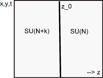
The quantum field theory which is dual to the D3-D7 system is a defect field theory consisting of Fermions confined to a 2-dimensional plane which separates 3-dimensional space into two regions as depicted in figure 1. The 3+1-dimensional bulk is occupied by supersymmetric Yang-Mills theory with gauge group SU(N) on one side of the defect and gauge group SU(N+k) on the other side of the defect. There are species of 2-component spinors of the 2+1-dimensional Lorentz group , living on the defect. In the conformal invariant solution this symmetry is extended to the 2+1-dimensional conformal group . The Fermions transform in the fundamental representation of a global symmetry. Since we consider no processes which use the non-abelian nature of , for simplicity we will take (and remember that to apply to graphene, we need to produce the correct flavor symmetry). The Fermions also transform in the fundamental representation of the gauge group of supersymmetric Yang-Mills theory which inhabits the 3+1-dimensional bulk of the space-time. The bulk Yang-Mills theory has different gauge groups on each side of the defect, as shown in figure 1. This is a result of the fact that, the D7-branes with internal fluxes which we shall use can be described as D7-branes with D3-branes dissolved into their worldvolumes. The D7-brane then forms a boundary between regions with different numbers of D3-branes and therefore different amounts of Ramond-Ramond 4-form flux, thus different ranks of the gauge group in the field theory dual.
We shall be interested in field theories which become parity and charge conjugation invariant in their high energy limit. This is what is expected in a class of condensed matter theories where the underlying dynamics is parity and particle-hole symmetric. These symmetries can be broken by deformations like external magnetic field, chemical potential or parity violating mass terms which are irrelevant in the ultraviolet limit but can be important to the infrared properties of the theory. On the D-brane side, imposing parity and charge conjugation symmetry will involve taking the appropriate boundary condition for the embedding of the D7-brane in as well as setting the fluxes equal, .
The paper is organized as follows: In Section 2 we review the embedding of the probe D7-brane in . In Section 3 we discuss the properties of the conformally invariant solution of the embedding problem. In Section 4 we discuss the solution with a chemical potential and charge density. In particular, we derive expressions for the Debye screening length at strong coupling, as functions of chemical potential and of density. In Section 5 we examine the same system with an external magnetic field in the special case that the charge density is tuned to zero. We find a simple expression for the diamagnetic moment of the system. We solve the embedding equation perturbatively in the ratio of condensate to magnetic field. We find a relationship between the mass and the chiral condensate to linear order in in equation (5.53). In Section 7 we show that turning on an infinitesimal charge density can also be taken into account perturbatively and we write the embedding equation to leading order in the filling fraction .
2 D7-brane
In the limit where the string theory is classical, the problem of embedding a D7-brane in the geometry reduces to that of finding an extremum of the Dirac-Born-Infeld and Wess-Zumino actions,
| (2.2) |
where is the closed string coupling constant, which is related to the Yang-Mills coupling by , are the coordinates of the D7-brane world-volume, is the induced metric, is the 4-form of the background, is the world-volume gauge field and the D7 brane tension is
| (2.3) |
We shall work with coordinates where the metric of the background space is
| (2.4) |
Here, are coordinates of the Poincare patch of . In our notation, and in natural units and , has the dimension of inverse length and have dimensions of length. is the radius of curvature. The boundary of is located at and the Poincare horizon at . The 5-sphere is represented by two unit 2-spheres, with polar coordinates and with coordinates . The 2-spheres are fibered over the interval . The Ramond-Ramond 4-form is
| (2.5) |
with obeying the equation
| (2.6) |
The dynamical variables are the ten functions of eight world-volume coordinates which embed the D7-brane in ,
as well as the eight worldvolume gauge fields
Parity and charge conjugation are important symmetries for the class of quantum field theory systems that we are interested in. For example, graphene is certainly parity invariant and, to a good approximation, it has particle-hole symmetry. We would expect to model it using field theories that have parity and charge conjugation symmetry. The string theory dual of such a field theory should also have these symmetries. We should therefore make sure that the problem of finding a minimum of the action (2.2) itself is symmetric. Parity in two dimensions is a reflection of one of the spatial coordinates, . This symmetry is usually broken by Wess-Zumino terms, which are111Note that we have presented the second Wess-Zumino term (2.8) in a form that is integrated by parts. This was to avoid specifying the integration constant in which would be obtained by integrating the expression in (2.6). Specifying that integration constant (which we shall do in the following) is regarded as string theory gauge fixing and physical quantities should not depend on it. We can think of our integration by parts in (2.8) as equivalent to adding a surface term to the Wess-Zumino term in order to restore this gauge invariance.
| (2.7) | ||||
| (2.8) |
Indeed, (2.7) changes sign when . We must therefore compensate the sign change by another change of the world-sheet variables, say . However, now (2.7) is invariant but (2.8) changes sign and is not invariant. We can also make it invariant by another change of variables, . (Note that is invariant and changes sign under this transformation.) Then, both of the Wess-Zumino terms are invariant, as is the Dirac-Born-Infeld action. In summary, our parity transformation is the replacement
| (2.9) | ||||
| (2.10) | ||||
| (2.11) |
Charge conjugation symmetry (C) is the replacement and the Wess-Zumino terms are invariant. However, we shall introduce a background field
| (2.12) |
Here, is the strength of the monopole bundle222A monopole bundle has quantized flux. Here the number of quanta is very large in the strong coupling limit , so that it is to a good approximation a continuously variable parameter. which is needed to stabilize the system. Note that, to be invariant under parity, (2.9)-(2.11), the fluxes on the 2-spheres have to be equal, . This is seen most clearly by noting that, in (2.9)-(2.11), the transformation interchanges the 2-spheres. The background field breaks a symmetry if the two components in the total field transform differently. Under C, . We shall need a definition of C so that . Such a transformation is
| (2.13) | ||||
| (2.14) |
Then (2.7) and (2.8) are invariant and (2.12) transforms covariantly under our definition of C. We have established that the mathematical problem of finding the D7 embedding has the discrete symmetries which will appear as C and P for the 2+1-dimensional Fermions. In the case of , this is clear, the worldsheet gauge field is dual to a conserved U(1) current for the Fermions and corresponds to , which is implemented by the usual C transformation of Fermi fields. For parity, this is also the case, the Fermion kinetic term is covariant under . However a 2-component Fermion mass operator changes sign under this parity transformation, so parity takes the place of chiral symmetry in 2+1-dimensions in that it protects the masslessness of Fermions. Indeed, the geometric argument of reference [33] explains that the deviation of the angle from its symmetric value corresponds to a separation of the D3 and D7 branes and a mass for the D3-D7 strings. At the same time, this deviation would violate parity.
Our Ansätz for a solution will describe a D7-brane covering the whole range of and it is for the most part determined by symmetry,
| (2.15) |
we will denote the coordinate by . The two unknown functions in this embedding are then and . Our Ansätz for the world-volume gauge fields is
| (2.16) |
where is a constant magnetic field which is proportional to a constant magnetic field in the dual field theory and is the temporal world-volume gauge field which must be non-zero in order to have a uniform charge density in the field theory dual.333 and are related to the physical magnetic field and charge density as , so that where the dimensionless parameter is the filling fraction of degenerate Landau levels.
With the Ansätz (2.15) and (2.16), the D7-brane world-volume metric is
| (2.17) |
where prime denotes derivative by . The Lagrangian is
| (2.18) |
where, using (2.3),
| (2.19) |
The factor of in the numerator comes from half of the volume of the unit 2-spheres (the other factors of 2 are still in the action). Since nothing depends on , the integral over these coordinates produces the volume factor which appears in . The Wess-Zumino term gives a source for , so that, as long as the flux is nonzero, will be non-zero and -dependent. Note that, since has dimension of length cubed and has the dimension of inverse length, the integral of (2) over will be dimensionless, as it should be.
Now, we must solve the equations of motion for the functions , and which result from the Lagrangian (2) and the variational principle. Since the Lagrangian depends only on their derivatives and not on the variables and themselves, and are cyclic variables and they can be eliminated using their equations of motion,
| (2.20) | ||||
| (2.21) |
where and are constants of integration. can be interpreted as being proportional to the pressure in the -direction and, by translation invariance, for a single brane, we would expect that it would be zero if the brane is not accelerating444The parameter becomes important when there is more than one brane, as the branes interact with each other and a pressure is required to hold them together, or apart, depending on their relative orientations [31]. With a single brane, because of translation invariance, this pressure must vanish.. It is also clear that, if the brane is to reach the Poincare horizon at , equation (2.20) will make sense there only if we set . Also, to get (2.21) we have integrated to get the term in the equation. We have taken the integration constant so that , so that it has the correct transformation property under P,
| (2.22) |
The overall constant of integration in (2.22) is, of course, a superstring gauge choice. Other choices would give equivalent results, but would alter what we mean by total charge density and would complicate the parity transformation law. Here, for simplicity, we make the choice given in (2.22). The integration constant is then proportional to the total charge density in the field theory dual. Moreover, we can solve for and ,
| (2.23) | ||||
| (2.24) |
We must then use the Legendre transformation
to eliminate and . We obtain the Routhian
| (2.25) |
which must now be used to find an equation of motion for . Applying the Euler-Lagrange equation to the Routhian (2.25) yields the equation of motion
| (2.26) |
where the overdot is the logarithmic derivative . In the next few Sections, we will discuss some of the solutions of this equation.
3 Conformal field theory
Let us first review the relevant solutions for the D7-brane geometry when the external magnetic field and the charge density vanish: . These are described in references [8] and [33]-[39]. The equation for is
| (3.27) |
In the large regime, we require that the angle approaches the parity symmetric solution, . We also note that the constant angle is an exact solution of equation (3.27). Linearizing about that solution yields the differential equation
| (3.28) |
which is solved by
| (3.29) |
where
| (3.30) |
The argument of the square root is non-negative and the exponents are real numbers if is large enough,
| (3.31) |
This is the parameter regime where mass term in the linearized equation (3.29) does not violate the Breitenholder-Freedman bound. In the regime , both and are positive, so that both solutions in (3.29) go to zero at . Moreover, when they are both positive, both solutions diverge at . Thus we see that there is no small deviation from the solution which is itself a solution. For this reason we call an isolated solution.
Let us discuss this in a little more detail. Regardless of its behavior at , if is to have a “normalizable mode” which remains finite at , for small values of , the solution must also go to a zero of the last term in (3.27). When , there are three zeros of the last term in (3.27), . The exponents of the linearized equation in the region , in each of the three cases are
| (3.32) | |||||
| (3.33) | |||||
| (3.34) |
Note that the exponent for fluctuations about the asymptotic which is given in (3.33) for the small regime is identical to the one in the large regime given in (3.30). The first solution would be acceptable only if both and are zero. The solution would then necessarily be a constant and violates the boundary condition at large , where should go to . If the boundary condition at infinity were different, so that the constant everywhere were a solution, this solution would describe a D5-brane with flux in this geometry [42]. This is an interesting possibility, but not the one that we need here.
The second solution (3.33) is the isolated solution. It is constant and isolated for the reasons that we have discussed above and it is the only solution that does not violate parity.
The third small solution is which is not isolated – since is negative and is positive, is allowed to be nonzero and we need in order to have good behavior at small . At large , both constants and in equation (3.29) are allowed to be nonzero, so the asymptotic behavior of the solutions is characterized by three nonzero constants, , and . Generically, for a fixed value of one of the constants, for example, , both and must be tuned to obtain . Then, and are functions of . This means that we have a 1-parameter family of solutions parameterized by . This parameter is the holographic dual of a parity violating Fermion mass term in the quantum field theory. The solution has a relevant parity violating operator with conformal dimension
which can be introduced and which has coupling constant dual to the parameter and expectation value dual to the parameter .555In an alternative quantization, if and are both greater than , the unitarity bound for conformal dimensions of operators in d=2+1, the roles and can be interchanged [43]. Turning on this operator preserves charge conjugation symmetry but breaks parity symmetry and it corresponds to making nonzero. Once is nonzero, no matter how small, the solution will evolve to the same value, at . This can be significantly different from the of the parity invariant solution. This has the interpretation of a renormalization group flow driven by a relevant operator. Note that, when , the exponents are . In the dual field theory this is interpreted as having the Fermion mass operator with dimension 3, that is, exactly marginal. In this case the angle goes to at small . A numerical solution of (3.27) is easy to find. Plots of numerical solutions exhibiting this behavior were given in reference [8].
4 Conformal field theory with charge density
We note from the Lagrangian (2) that it contains a cubic term . Remember that is and violating, is P and C violating and is P and CP violating. This implies that turning on any two of these fields will violate all three of the symmetries , and and, in the equation of motion, turning on two will produce a source for the third. In the following sections we will discuss the situation when all three are turned on. Before that, let us examine what happens when only one of the three is turned on. In the above, we have already discussed one of the cases, the situation when and are turned off but could be a function of . That solution violated parity but preserved charge conjugation invariance. In this section, we will keep a constant, set to zero and turn on . This solution violates charge conjugation invariance, in that there is a fixed non-zero charge density, but it is invariant under parity. What we obtain is a sector of the conformal field theory where the charge density is fixed to a particular value proportional to . The equation for is gotten from (2.26) by setting ,
| (4.35) |
We see that is a solution of this equation. The remaining embedding functions can be found from by integrating the expressions in (2.23) and (2.24) with and ,
| (4.36) | ||||
| (4.37) |
Note that the range of these functions is finite.
The chemical potential is given by difference in the value of the gauge field at and (where we remember the normalization in (2.16))
| (4.38) |
is Euler’s beta-function. Now, remembering that the charge density is defined by , we can write the expression for the charge density as a function of the chemical potential,
| (4.39) |
For a generic value of in the range of interest, say ,
| (4.40) |
One might compare this with the free field theory where
| (4.41) |
The scaling with is a consequence of conformal invariance. In a theory where the U(1) current is conserved, the Debye screening mass (the inverse of the Debye screening length) can be derived from the charge density-chemical potential relationship by taking a derivative of the charge density by the chemical potential[44],
| (4.42) |
It is interesting that coefficients of in the strongly coupled theory and the free field theory and the Debye screening lengths differ by a factor of which can be significant in the large limit. The Debye screening length as a function of gate voltage is a quantity which could in principle be measured in a relativistic condensed matter system such as graphene. The coupling constant could also be varied, in principle, by changing the dielectric constant of the vicinity of the material. Such a measurement would be an interesting test of the hypothesis that the relativistic material could be in a strongly correlated state that is described by a conformal field theory similar to the one which solves the D3-D7 model.
5 Conformal field theory in a magnetic field
The equation for the angle with and is
| (5.43) |
This equation is solved by . The magnetization as a function of field is given by the derivative of the vacuum energy by the field,
| (5.44) |
where we have recognized that the energy as a function of field is simply the negative on-shell Routhian, which we can find by setting , in (2.25). We obtain
| (5.45) |
The above integral diverges. It can be defined by subtracting the energy from it. Then the result is finite. Then, the derivative by the field renders the remaining integral finite,
| (5.46) |
The sign, is a result of diamagnetism, which is what is expected for electrons in a magnetic field. We can compare this with the result for free Fermions. There, all negative energy states are occupied and their spectrum in a magnetic field is that of relativistic Landau levels, given by , with . The degeneracy of each Landau level is . The ground state energy is
where we have defined the infinite sum by zeta-function regularization and the value of the zeta-function is . The vacuum energy is positive and
| (5.47) |
It is again interesting that the diamagnetism of strongly and weakly interacting Fermions differ by a factor of .
Now, we observe that, with a finite magnetic field, at , the angle must solve the equation
| (5.48) |
The only solution of this equation is , which fixes the value that must take at . However, if we study the linearized equation in this region, we find that, unlike the case that we studied in the previous sections where the constant was an isolated solution, here, it is not isolated. There are solutions close by where depends on and approaches when goes to zero and infinity. To see this, the linearized equation in the small region is
| (5.49) |
and it has solutions
| (5.50) |
We see that the solution (5.50) converges to if we choose the constant . This requires tuning the asymptotic behavior of the solution at large , which we shall examine in more detail in the following. In this way, we see that, when there is a magnetic field present, there are solutions of the equation for which are infinitesimally close to the constant for all values of . This is in contrast to the case without a magnetic field where any infinitesimal deviation of from at large led to a non-infinitesimal deviation at small . In the present case with magnetic field, we can study solutions which deviate from by a small amount perturbatively. We shall spend the remainder of this section studying the properties of these solutions.
Before we begin, we note that, as soon as deviates from the constant , the solution violates all three of the discrete symmetries, parity, charge conjugation and CP. That it violates C and CP can be seen from the equation (2.24) which requires to be non-zero, at least for intermediate values of . However, we are still free to set the parameter , and therefore the charge density to zero. In the next Section, we will examine what happens when we turn on a of infinitesimal magnitude.
In the appendix, we have studied (5.43) perturbatively. Parameterizing the asymptotic behavior of by two parameters and , , we found that they are related to each other in the following way
| (5.53) |
where and are given by
| (5.54) |
In equation (5.53) we see that the function changes in character as is varied from below to above the value at which . In fact, as depicted in figure 2, the function is discontinuous there. The behavior resembles a quantum phase transition - for a fixed value of , jumps in a discontinuous way as is varied. We note that this special value is just the value where the exponents and , which are interpreted as scaling dimensions of the chiral condensate and mass parameter, both obey the lower bound on dimensions that is required in a unitary conformal field theory, they have values . At that bound, an alternative quantization sets in. When , there is an alternative quantization where the interpretation of the mass and chiral condensate are interchanged, whereas when , the quantization that we describe is unique.
We note one other interesting behavior which occurs as is varied.
When it achieves a value , so that , the ratio
in (5.53) seems to diverge. This behavior is
depicted in figure 2. We interpret it as the
condensate remaining non-zero as is put to zero, that is,
spontaneous symmetry breaking, the presence of a nonzero condensate
when the source is put to zero. In addition, at this point, the sign
of the condensate versus the sign of the magnetic field flips, for
the sign of and the sign of are identical, for
the signs are opposite.
Here we have assumed that and are small parameters (in magnetic field units). This has allowed us to linearize and solve the equation for for all values of r. The existence of a value of at which but may differ from zero is a result of this analysis. We comment here that the result is possibly more robust and could well persist beyond our linear approximation. This follows from the fact that, if we fix and solve the theory to extract for differing values of , we find that generically varies smoothly and changes sign as is swept across the domain . This means that has a zero at some value of . In the linearized limit, becomes a linear function of and we see that the zero occurs at
We have found that the conformal dimensions of the operator which is dual to fluctuations of the angle lie in an interesting range when . A summary of some special values of in this range are given in Table 2.
| , | ||
|---|---|---|
| stability bound | ||
| classical dimensions | ||
| unitarity bound | ||
| 0 | chiral symmetry breaking | |
| marginal |

6 Finite density in presence of magnetic field
As we have remarked in the previous sections, the equation of motion (2.26) has the constant solution only when either , or both. When both and are nonzero, there is no constant solution. When and were set to zero, we saw that the constant solution was isolated. As soon as we turn on a non-constant behavior of at , the solution near deviates by a large amount from . Then, in the previous section, we found that when is nonzero, but we still tune to zero, the constant solution is no longer isolated and we explicitly found a solution which differs from the constant by a small amount for all values of . In this Section, we shall examine what happens when we turn on a small value of .
In the small region, the non-constant solution must go to a zero of the last term in (2.26). That is, it must solve the equation
| (6.55) |
When , this equation is solved by , and the constant solution is allowed and, as we saw in the previous section, even when it is not constant, approached when approaches either 0 or . Now, when is nonzero, this is no longer the case, there is no constant solution and the non-constant must approach a zero of (6.55) which is no longer . If we consider the case where is small, it is solved by
| (6.56) |
It is consistent that the deviation of from is of order . If we consider
| (6.57) |
and Taylor expand (2.26) to first order in and , we obtain equation (A.74), which we recopy here for the reader’s convenience:
| (6.58) |
The solution of the (6.58) is given by
| (6.59) |
where is the general homogenous solution and is the Green function. The Green function is given by
| (6.60) |
where is the regular solution at origin, is the regular solution at the boundary and is the step function. Having only one regular solution at the origin, we are forced to choose the linear combination of and that we found in (A.95) . Both of and are regular at the boundary and vanish. We specify the solution by specifying the boundary condition at so that the Green function part does not contribute to the coefficient of term that dies slower, ; so, we choose to be . We are just left to find the right normalization of our Green function so that
| (6.61) |
where the primes are differentiation with respect to . This equation can be written as
| (6.62) |
Integrating the above equation, we get the following constraint
| (6.63) |
which can be written as
| (6.64) |
where is the Wronskian. The (6.62) has a form of Sturm-Liouville equation. It is a well-known property of such an equation that the Wronskian of the solutions is given by
| (6.65) |
which ensures that we can satisfy the constraint in (6.64). We just need to evaluate the Wronskian at a given point to fix the normalization. Substituting the asymptotic expansions of and , we get
| (6.66) |
Now we can use (6.66) to find the Wronskian. Using the linear combination (A.95) as , we find that the Wronskian is given by
| (6.67) |
So, we need to define in the following way to get the right normalization
| (6.68) |
Putting all the parts together, we can finally write the complete expression of
| (6.69) |
where is the solution to homogeneous equation and the rest are as listed below:
| (6.70) |
| (6.71) |
| (6.72) |
In this section, we have derived an explicit solution of equation of motion in presence of magnetic field and finite density. This solution shows finite deviation from constant solution.
7 Conclusions
In this Paper, we have examined a regime where a mass operator, magnetic field and charge density can be turned on and the modification of the D3-D7 conformal field theory can be studied perturbatively. In Sections 5 and 6 we solved the leading perturbation explicitly. For this solution, we can compute the relationship between the coefficient of the mass operator and the chiral condensate for interesting values of . This function is depicted in figure 2. It has the interesting feature that, at , the relationship becomes singular. We interpret the singularity as a signal of spontaneous symmetry breaking.
Moreover, as a byproduct, we have found holographic expressions for the Debye screening length as a function of fermion density and of the diamagnetic moment of the ground state as a function of magnetic field. They both exhibit a dependence on the charge density and magnetic field consistent with scale symmetry. They also have a mild dependence on the coupling constant which could in principle be interesting to compare with a real material, such as graphene where these quantities can be measured. It would be interesting to check the functional form in order to test the hypothesis that graphene is scale invariant. It would also be interesting to see whether these quantities in graphene differ in any significant way from the free field expressions, and whether the deviation is in the same direction as predicted by the strong coupling formula.
Appendix A Appendix
We begin by considering a solution of equation (5.43) which deviates from the constant by a small amount,
| (A.73) |
and Taylor expand (2.26) to first order in and , we obtain
| (A.74) |
which we shall now try to solve over the full range of . Note that (A.74) reduces to our small linearization in (5.50) at . The transformation
| (A.75) |
puts (A.74) in the following form, which in the case of is the standard form of the associated Legendre equation
| (A.76) |
where the parameters are
| (A.77) |
For future reference, we note that is always positive but can change sign. One can write in terms of as
| (A.78) |
| (A.79) |
The Legendre equation has the general solution
| (A.80) |
The associated Legendre functions are given by Hypergeometric functions as below
| (A.81) |
| (A.82) |
where we have defined phases so that the functions are real for . Both of the solutions (A.81) and (A.82) diverge at (which corresponds to ) and converge to zero at (which corresponds to ).
To find a solution which is finite at , we need to adjust the two constants, and in (A.80) so that the singularity cancels. Since corresponds to , we shall need to study in the regions where for and for , respectively. It is easy to study near . From the definition of Hypergeometric functions,
| (A.83) |
we see that the leading term in the series is normalized to one,
| (A.84) |
Then, from (A.81), we see that the asymptotic behavior of is given by
| (A.85) |
Now, let us consider . We note that, for the values of and of interest, is divergent at . Since the asymptotic small behavior of the solutions of the Legendre equations exhibit only one divergent solution, we know from the outset that the divergent nature of must be similar to that of .
Euler’s formula is an integral representation of which is valid when and ,
| (A.86) |
Using it, one can show that
| (A.87) |
Using the same representation one can show that if
| (A.88) |
for the above result can be generalized using analytical continuation.
In our case of interest, in Eq. (A.82) has
| (A.89) | |||
| (A.90) |
which is not in the domain of applicability of (A.88). If we use the transformation (A.87), we can change the arguments of so that (A.88) can be applied. Then we get
| (A.91) |
where, now
| (A.92) |
The result is
| (A.93) |
and we find the asymptotic behavior of ,
| (A.94) |
which shows the expected divergent behavior. Then the regular solution turns out to be (A.80) (which we recopy here)
where and are related by
| (A.95) |
We have now found an acceptable non-singular solution in the small regime. It is given by equation (A.80) with the constants related by (A.95). We now need to find what this implies for the large behavior of the solution. In particular, it should fix the relationship between the coefficients of the two asymptotic behaviors of the solution at large which are displayed in equation (3.29), that is, it should fix the relationship between and . For large one gets
| (A.96) |
Using the same integral representation (A.86), one can show that
| (A.97) |
For in the regime where we get
| (A.98) | ||||
Because , then we find that , which allows us to use (A.88). Using the identity (A.88), we find that
| (A.100) |
Another identity that we shall use is the following identity
| (A.101) |
Using this identity, we see that the second term in (LABEL:taylorexp) can be written as
| (A.102) |
Now, we should be more careful because for , we can not use the integral representation (A.86). In this case and the (A.88) can not be used. We shall therefore consider the two cases and separately:
| (A.103) |
Then one has
| (A.104) |
where the terms that fall off as get canceled by each other (as one expects from the asymptotic solutions of (A.76) for large values of ).
To deal with the case we can not use the Taylor expansion directly, as the derivative of at diverges. From the asymptotic solutions of (A.76), we know that to the two highest orders, can either go like or . The part is easy to find, we can just use the (A.98), and look at . If we subtract the term from , because vanishes at infinity, the result would vanish at infinity. Considering this fact, we find the following limit
| (A.105) |
which can be used to find the coefficient of term in (the extra power of is because of presence of in (LABEL:taylorexp)). Using (A.102), (A.87)and (A.88), we find that
| (A.106) |
where comes from the chain rule used to change the variable of differentiation.
So we find that for , can be written as
| (A.107) |
Plugging in the above results in (A.98), we find the following asymptotic expansion of
| (A.108) |
where we have used the fact that .
We neglect the term, as it belongs to next orders. We then have the following simplified equation of for
| (A.109) |
Around the normalizable/un-normalizable nature of the two terms switches. Later, we will explore the behaviour of the solution around , and see if there is anything special about this point.
Now we shall study near the boundary, . We Taylor expand by using the fact that and (A.102), which result in
| (A.110) |
we find that
| (A.111) |
We expect to find the asymptotic behavior (3.29), that is, . Here, the correct powers of are found by
| (A.112) |
| (A.113) |
where the extra factor of comes from definition of in (A.80).
The first asymptotic term (with ), which decays slower, always comes from .
| (A.114) |
The term is coming from the fact that is defined in terms of but the Legendre Functions are in terms of .
Depending on the sign of , the second asymptotic term (with ) may come from either or from both of and . If , the second term in goes at most like and first term in goes like , because , the term coming from is the dominant one. (We recall that and .)
Looking for the coefficients, one finds that
| (A.115) |
then
| (A.116) |
If , we use the expansion we found for and at , which results in
| (A.117) |
then
| (A.118) |
References
- [1] J. M. Maldacena, Adv. Theor. Math. Phys. 2, 231 (1998); S. S. Gubser, I. R. Klebanov, A. M. Polyakov, Phys. Lett. B428, 105 (1998); E. Witten, Adv. Theor. Math. Phys. 2, 253 (1998)253291.
- [2] S. Hartnoll, Class. Quant. Grav. 26, 224002 (2009) arXiv:0903.3246; M. Rangamani, Class. Quant. Grav. 26, 224003 (2009) arXiv:0905.4352; J. McGreevy, arXiv:0909:0518.
- [3] G. W. Semenoff, Phys. Rev. Lett. 53 2449 (1984).
- [4] A. K. Geim, K. S. Novoselov, Nat. Mater. 6 183 (2007); K. Novoselov, Nature Materials 6 720 - 721 (2007); M. I. Katsnelson, Materials Today 10 20 (2007); G. W. Semenoff, Phys. Scripta T146, 014016 (2012) [arXiv:1108.2945 [hep-th]]. .
- [5] C. L. Kane, E. J. Mele, Phys. Rev. Lett. 95,146802 (2005); B. A. Bernevig, T. L. Hughes, S.-C. Zhang, Science 314 1757-1761 (2006); L. Fu, C. L. Kane, Phys. Rev. B 76 045302 (2007); C. Nayak, S. H. Simon, A. Stern, M. Freedman, and S. Das Sarma, Rev. Mod. Phys. 80, 1083 (2008).
- [6] L. Balents, M. P. A. Fisher, C. Nayak, Int. J. Mod. Phys. 10, 1033 (1998); M. Franz, Z. Teanovi, Phys. Rev. Lett. 87, 257003 (2001); I. Herbut, Phys. Rev. B66, 094504 (2002).
- [7] J. Ruostekoski, G.V. Dunne, J. Javanainen, Phys. Rev. Lett. 88, 180401 (2002); S.-L. Zhu1, B. Wang, L.-M. Duan, Phys. Rev. Lett. 98, 260402 (2007); L. Lepori, G. Mussardo and A. Trombettoni, arXiv:1004.4744 [hep-th]
- [8] J. L. Davis, H. Omid and G. W. Semenoff, “Holographic Fermionic Fixed Points in d=3,” JHEP 1109, 124 (2011) [arXiv:1107.4397 [hep-th]].
- [9] K.G. Klimenko, Theor. Math. Phys. 89, 1161 (1992).
- [10] V.P. Gusynin, V.A. Miransky, I.A. Shovkovy, Phys. Rev. Lett. 73 (1994) 3499 [hep-ph/9405262].
- [11] V.P. Gusynin, V.A. Miransky, I.A. Shovkovy, Phys. Rev. D 52 (1995) 4718 [hep-th/9407168].
- [12] G. W. Semenoff, I. A. Shovkovy and L. C. R. Wijewardhana, Mod. Phys. Lett. A 13, 1143 (1998) [arXiv:hep-ph/9803371].
- [13] G. W. Semenoff, I. A. Shovkovy and L. C. R. Wijewardhana, Phys. Rev. D 60, 105024 (1999) [arXiv:hep-th/9905116].
- [14] G. W. Semenoff and F. Zhou, JHEP 1107, 037 (2011) [arXiv:1104.4714].
- [15] E. V. Gorbar, V. P. Gusynin, V. A. Miransky and I. A. Shovkovy, [arXiv:1105.1360].
- [16] O. V. Gamayun, E. V. Gorbar and V. P. Gusynin, [arXiv:1206.2266].
- [17] I. A. Shovkovy,
- [18] V. G. Filev, C. V. Johnson and J. P. Shock, JHEP 0908, 013 (2009) [arXiv:0903.5345 [hep-th]].
- [19] R. C. Myers and M. C. Wapler, JHEP 0812, 115 (2008) [arXiv:0811.0480 [hep-th]].
- [20] N. Evans and E. Threlfall, Phys. Rev. D 79 (2009) 066008 [arXiv:0812.3273 [hep-th]].
- [21] V. G. Filev, JHEP 0911, 123 (2009) [arXiv:0910.0554 [hep-th]].
- [22] N. Evans, A. Gebauer, K. Y. Kim and M. Magou, JHEP 1003, 132 (2010) [arXiv:1002.1885 [hep-th]].
- [23] K. Jensen, A. Karch, D. T. Son and E. G. Thompson, Phys. Rev. Lett. 105, 041601 (2010) [arXiv:1002.3159 [hep-th]].
- [24] N. Evans, A. Gebauer, K. Y. Kim and M. Magou, Phys. Lett. B698, 91 (2011). [arXiv:1003.2694 [hep-th]].
- [25] S. S. Pal, Phys. Rev. D82, 086013 (2010). [arXiv:1006.2444v4 [hep-th]].
- [26] N. Evans, K. Jensen, K.-Y. Kim, Phys. Rev. D82 105012 (2010)[arXiv:1008.1889 [hep-th]].
- [27] S. Bolognesi and D. Tong, arXiv:1110.5902 [hep-th].
- [28] S. Bolognesi, J. N. Laia, D. Tong and K. Wong, JHEP 1207, 162 (2012) [arXiv:1204.6029 [hep-th]].
- [29] G. Grignani, N. Kim and G. W. Semenoff, arXiv:1203.6162 [hep-th].
- [30] F. Preis, A. Rebhan and A. Schmitt, JHEP 1103, 033 (2011) [arXiv:1012.4785 [hep-th]].
- [31] J. L. Davis and N. Kim, JHEP 1206, 064 (2012) [arXiv:1109.4952 [hep-th]].
- [32] S.-J. Rey, Prog. Theor. Phys. 177, 128 (2009).
- [33] O. Bergman, N. Jokela, G. Lifschytz and M. Lippert, JHEP 1010, 063 (2010) [arXiv:1003.4965 [hep-th]].
- [34] N. Jokela, G. Lifschytz and M. Lippert, JHEP 1102, 104 (2011) [arXiv:1012.1230 [hep-th]].
- [35] N. Jokela, M. Jarvinen and M. Lippert, JHEP 1105, 101 (2011) [arXiv:1101.3329 [hep-th]].
- [36] O. Bergman, N. Jokela, G. Lifschytz and M. Lippert, Fortsch. Phys. 59, 734 (2011).
- [37] O. Bergman, N. Jokela, G. Lifschytz and M. Lippert, JHEP 1110, 034 (2011) [arXiv:1106.3883 [hep-th]].
- [38] N. Jokela, M. Jarvinen and M. Lippert, JHEP 1201, 072 (2012) [arXiv:1107.3836 [hep-th]].
- [39] N. Jokela, G. Lifschytz and M. Lippert, JHEP 1205, 105 (2012) [arXiv:1204.3914 [hep-th]].
- [40] J. Gonzalez, F. Guinea. M. A. H. Vozmediano, Nucl. Phys. B. 424, 595 (1994); Phys. Rev. B 59, R2474 (1999); E. V. Gorbar, V. P. Gusynin, V. A. Miransky, Phys. Rev. D 64, 105028 (2001); E. V. Gorbar, V. P. Gusynin, V. A. Miransky, I. A. Shovkovy, Phys. Rev. B66, 045108 (2002); D.E. Sheehy, J. Schmalian, Phys. Rev. Lett. 99, 226803 (2007); O. Vafek, M. J. Case, Phys. Rev. B 77, 033410 (2008); Igor F. Herbut, Vladimir Juricic’, Oskar Vafek, Phys. Rev. Lett. 100 (2008) 046403; Vladimir Juricic’, Igor F. Herbut, Gordon W. Semenoff, Phys.Rev.B 80, 081405, (2009); Igor F. Herbut, Vladimir Juricic’, Oskar Vafek, Phys.Rev.B 82, 235402, (2010).
- [41] D. Kutasov, J. Lin, A.Parnachev, arXiv:1107.2324 [hep-th].
- [42] G. Grignani, N. Kim and G. W. Semenoff, “D3-D5 Holography with Flux,” arXiv:1203.6162 [hep-th].
- [43] I. R. Klebanov and E. Witten, Nucl. Phys. B 556, 89 (1999) [arXiv:hep-th/9905104].
- [44] E. S. Fradkin, Proc. of the Lebedev Physics Institute, 29, 6 (1965).
- [45] George E. Andrews, Ranjan Roy, Richard Askey, “Special Functions” Encyclopedia of Mathematics and its Applications, The University Press, Cambridge, 1999.