Optical imaging of phantoms from real data by an approximately globally convergent inverse algorithm

Abstract

A numerical method for an inverse problem for an elliptic equation with the running source at multiple positions is presented. This algorithm does not rely on a good first guess for the solution. The so-called “approximate global convergence” property of this method is shown here. The performance of the algorithm is verified on real data for Diffusion Optical Tomography. Direct applications are in near-infrared laser imaging technology for stroke detection in brains of small animals.

65B21; 65D10; 65F10

1 Introduction

We consider a Coefficient Inverse Problem (CIP) for a partial differential equation (PDE) - the diffusion model with the unknown potential. The boundary data for this CIP, which model measurements, are originated by a point source running along a part of a straight line. This PDE governs light propagation in a diffusive medium, such as, e.g. biological tissue, smog, etc.. Thus, our CIP is one of problems of Diffusion Optical Tomography (DOT). We are interested in applications of DOT to the detection of stroke in small animals using measurements of near infrared light originated by lasers. Hence, the above point source is the light source in our case. The motivation of imaging of small animals comes from the idea that it might be a model case for the future stroke detection in humans, at least in brains of neonatals, via DOT. We apply our numerical method to a set of real data for a phantom medium modeling the mouse’s brain. Although this algorithm was developed in earlier publications [17, 24, 25, 26] of this group, its experimental verification is new and is the main contribution of this paper.

As to our numerical method, we introduce a new concept of the “approximate global convergence” property. In the previous publication [17] of this group about this method the approximate global convergence property was established in the continuos case. Compared with [17], the main new analytical result here is that we establish this property for the more realistic discrete case. In the convergence analysis of [17] the Schauder theorem [14] was applied for $C^{2+\alpha}-$solutions of certain elliptic equations arising in our method. Now, however, since we consider the discrete case, we use the Lax-Milgram theorem. Here and below $C^{k+\alpha}$ are Hölder spaces [14], where $k\geq 0$ is an integer and $\alpha\in\left(0,1\right)$.

CIPs are both nonlinear and ill-posed. These two factors cause very serious challenges in their numerical treatments. Indeed, corresponding least squares Tikhonov regularization functionals usually suffer from multiple local minima and ravines. As a result, conventional numerical methods for CIPs are locally convergent ones, see, e.g. [4] and references cited there. To have a guaranteed convergence to a true solution, a locally convergent algorithm should start from a point which is located in a small neighborhood of this solution. However, it is a rare case in applications when such a point is known. The main reason why our method avoids local minima is that it uses the structure of the underlying PDE operator and does not use a least squares functional.

Therefore, it is important to develop such numerical methods for CIPs, which would have a rigorous guarantee of providing a point in a small neighborhood of that exact solution without any a priori knowledge of this neighborhood. It is well known, however, that the goal of the development of such algorithms is a substantially challenging one. Hence, it is unlikely that such numerical methods would not rely on some approximations. This is the reason why the notion of the approximate global convergence property was introduced in the recent work [19]; also see section 1.1.2 of the book [9] and subsection 4.1 below. The verification of our approximately globally convergent numerical method on computationally simulated data was done in [17, 24, 25, 26]. In this paper we make the next step: we verify this method on real data. Regardless on some approximations we have here, the main point is that our numerical method does not rely on any a priori knowledge of a small neighborhood of the exact solution.

In [6, 7, 8, 18, 19, 20] a similar numerical method for CIPs for a hyperbolic PDE was developed. These results were summarized in the book [9]. In particular, it was demonstrated numerically in Test 5 of [6], section 8.4 of [18], on page 185 of [9] and in section 5.8.4 of [9] that the approximately globally convergent method of [6, 7, 8, 18, 19, 20] outperforms such locally convergent algorithms as quasi-Newton method and gradient method. The main difference of the technique of these publications with the one of the current paper is in the truncation of a certain integral. In [6, 7, 8, 18, 19, 20] that integral was truncated at a high value $\overline{s}>0$ of the parameter $s>0$ of the Laplace transform of the solution of the underlying hyperbolic PDE. Indeed, in the hyperbolic case the truncated residual of that integral, which we call the “tail function”, is $O\left(1/\overline{s}\right)$, as $\overline{s}\rightarrow\infty$, i.e. this residual is automatically small in this case. Being different from the hyperbolic case, in the elliptic PDE with the source running along a straight line, $\overline{s}>0$ represents the distance between the source and the origin. Because of this, the tail function is not automatically small in our case. Thus, a special effort to ensure this smallness was undertaken in [17], and is repeated in the current publication. It was shown numerically in [17] that this special effort indeed improves the quality of the reconstruction, compare Figures 2b and 2c in [17].

Our real data were collected at the boundary of a 2-D cross-section of the 3-D domain of interest, see section 6. Hence, we have imaged this cross-section only and have ignored the dependence on the third variable. In addition, our theory requires the use of many sources placed along a straight line. However, limitations of our experimental device allow us to use only three sources on this line. We believe that the accuracy of our results (Table 8.2) confirms the validity of both these assumptions as well as manifests a well known fact that there are always some discrepancies between the analysis and computational studies of numerical methods.

Because of the above mentioned substantial challenges, the topic of the development of non-locally convergent numerical methods for CIPs is currently in its infancy. As to such methods for CIPs for elliptic PDEs, we refer to, e.g. publications [2, 11, 15, 21, 22, 23] and references cited there. These publications are concerned with the Dirichlet-to-Neumann map (DN). We are not using the DN here.

In a general setting, an ill-posed problem is a problem of solving an equation $F\left(x\right)=y$  with a compact operator $F$. Here $x\in B_{1}$, $y\in B_{2},$ where $B_{1}$ and $B_{2}$ are certain Banach spaces. Naturally, the operator $F$ varies from one problem to another one. It is well known that the existence theorem for such an equation is very tough to prove, since the range of any compact operator is ‘too narrow’ in certain sense, see, e.g. Theorem 1.2 in [9]. Therefore, by one of fundamental concepts of the theory of Ill-Posed Problems, one should assume the existence of an exact solution of such a problem for the case of an “ideal” noiseless data [5, 9, 27]. Although this solution is never known in practice and is never achieved in practice (because of the noise in the real data), the regularization theory says that one needs to construct a good approximation for it. We assume that our CIP has an exact solution for noiseless data and also assume that this solution is unique.

The rest of this paper is arranged as follows. In section 2 we pose both forward and inverse problems and study some properties of the solution of the forward problem. In section 3 we present our numerical method. In section 4 we conduct the convergence analysis. In section 5 we discuss the numerical implementation of our method. In section 6 we describe the experiment. In section 7 we outline our procedure of processing of real data. In section 8 we present reconstruction results. We briefly summarize results in section 9.

2 Statement of the Problem

2.1 The Inverse Problem

Below  $\mathbf{x}=\left(x,z\right)\in\mathbb{R}^{2}$ and $\Omega\subset$ $\mathbb{R}^{2}$ is a convex bounded domain. The boundary of this domain $\partial\Omega\in C^{3}$ in our analysis. In numerical studies $\partial\Omega$ is piecewise smooth. Consider the following elliptic equation in $\mathbb{R}^{2}$ with the solution vanishing at infinity,

$$\Delta u-a\left(\mathbf{x}\right)u = -\delta\left(\mathbf{x}-\mathbf{x}_{0}\right),\mathbf{x},\mathbf{x}_{0}\in\mathbb{R}^{2},$$ (1)

$$\underset{\left|\mathbf{x}\right|\rightarrow\infty}{\lim}u\left(\mathbf{x},\mathbf{x}_{0}\right) = 0.$$ (2)

Inverse Problem. Let $k=const.>0$. Suppose that in (1) the coefficient $a\left(\mathbf{x}\right)$ satisfies the following conditions

$$a\in C^{1}\left(\mathbb{R}^{2}\right),\text{ }a\left(\mathbf{x}\right)\geq k^{2}\text{ and }a\left(\mathbf{x}\right)=k^{2}\text{ for }\mathbf{x}\in\mathbb{R}^{2}\diagdown\Omega.$$ (3)

Let $L\subset\left(\mathbb{R}^{2}\diagdown\overline{\Omega}\right)$ be a straight line and $\Gamma\subset L$ be an unbounded and connected subset of $L$. Determine the function $a\left(\mathbf{x}\right)$ inside of the domain $\Omega,$ assuming that the constant $k$ is given and also that the following function $\varphi\left(\mathbf{x},\mathbf{x}_{0}\right)$ is given

$$u\left(\mathbf{x,x}_{0}\right)=\varphi\left(\mathbf{x,x}_{0}\right),\forall\left(\mathbf{x,x}_{0}\right)\in\partial\Omega\times\Gamma.$$ (4)

We are unaware about a uniqueness theorem for this inverse problem. Nevertheless, because of the above application, it is reasonable to we develop a numerical method. Thus, we assume that uniqueness for this problem holds. Our numerical studies of both the past [17, 24, 25, 26] and the current publication indicate that a certain uniqueness theorem might be established.

We assume that sources $\left\{\mathbf{x}_{0}\right\}$ are located outside of the domain of interest $\Omega$ because this is the case of our measurements and because we do not want to work with singularities in our numerical method. The CIP (1)-(4) has an application in imaging using light propagation in a diffuse medium, such as biological tissues. Since the modulated frequency equals zero in our case, then this is the so-called continuous-wave (CW) light. The coefficient $a\left(\mathbf{x}\right)=3\left(\mu_{s}^{\prime}\mu_{a}\right)\left(\mathbf{x}\right),$ where $\mu_{s}^{\prime}\left(\mathbf{x}\right)$ is the reduced scattering coefficient and $\mu_{a}\left(\mathbf{x}\right)$ is the absorption coefficient of the medium [3, 4]. In the case of our particular interest in stroke detections in brains of small animals, the area of an early stroke can be modeled as a small sharp inclusion in an otherwise slowly fluctuating background. Usually the inclusion/ background contrast $a_{incl}/a_{b}\geq 2.$ Therefore our focus is on the reconstruction of both locations of sharp small inclusions and the values of the coefficient $a\left(\mathbf{x}\right)$ inside of them, rather than on the reconstruction of slow changing background functions.

2.2 Some Properties of the Solution of the Forward Problem (1), (2)

2.2.1 Existence and uniqueness

First, we state the existence and uniqueness of the solution of the forward problem (1), (2). For brevity we consider only the case $\mathbf{x}_{0}\notin\overline{\Omega},$ since this is the case of our Inverse Problem. Let $K_{p}\left(z\right),z\in\mathbb{R},p\geq 0$ be the Macdonald function. It is well known [1] that for $y\in\mathbb{R}$

$$K_{p}\left(y\right)=\frac{\sqrt{\pi}}{\sqrt{2y}}e^{-y}\left(1+O\left(\frac{1}{y}\right)\right),y\rightarrow\infty.$$ (5)

Theorem 2.1.

Let $\Omega\subset\mathbb{R}^{2}$ be the above bounded domain. Assume that the coefficient $a\left(\mathbf{x}\right)$ satisfies conditions (3). Then for each source position $x_{0}\in\mathbb{R}^{2}\diagdown\overline{\Omega}$ there exists unique solution $u\left(\mathbf{x,x}_{0}\right)$ of the problem (1), (2) such that

$$u\left(\mathbf{x,x}_{0}\right)=\frac{1}{2\pi}K_{0}\left(k\left|\mathbf{x-x}_{0}\right|\right)+\widehat{u}\left(\mathbf{x,x}_{0}\right):=u_{0}\left(\mathbf{x-x}_{0}\right)+\widehat{u}\left(\mathbf{x,x}_{0}\right),$$ (6)

where the function $u_{0}$ is the fundamental solution of equation (1) with $a\left(\mathbf{x}\right)\equiv k^{2},$ the function $\widehat{u}$ satisfies (2), $\widehat{u}\in H^{2}\left(\mathbb{R}^{2}\right)$ and $\widehat{u}\in C^{2+\alpha}\left(\mathbb{R}^{2}\right).$ In addition, $u\left(\mathbf{x,x}_{0}\right)>0,\forall x\in\overline{\Omega}.$

A similar result for the 3-D case was proven in [9], see Theorem 2.7.2 in this reference. Hence, we leave out the proof of Theorem 2.1 for brevity.

2.2.2 The asymptotic behavior at $\left|\mathbf{x}_{0}\right|\rightarrow\infty$

It follows from (5) and (6) that the asymptotic behavior of the function $u_{0}\left(\mathbf{x-x}_{0}\right)$ is

$$u_{0}\left(\mathbf{x-x}_{0}\right) = w_{0}\left(\left|\mathbf{x}_{0}\right|\right)\left(1+O\left(\frac{1}{\left|\mathbf{x}_{0}\right|}\right)\right),\left|\mathbf{x}_{0}\right|\rightarrow\infty,$$

$$w_{0}\left(\left|\mathbf{x}_{0}\right|\right) = \frac{e^{-k\left|\mathbf{x}_{0}\right|}}{2\sqrt{2\pi\left|\mathbf{x}_{0}\right|}}.$$

Denote $b\left(\mathbf{x}\right)=a\left(\mathbf{x}\right)-k^{2}$. Then by (3) $b\left(\mathbf{x}\right)=0$ for $\mathbf{x}\in\mathbb{R}^{2}\diagdown\Omega$. Let $M_{1}$ be a positive constant. Denote

$$B\left(M_{1}\right)=\left\{b\in C^{1}\left(\mathbb{R}^{2}\right):\left\|b\right\|_{C^{1}\left(\overline{\Omega}\right)}\leq M_{1},b\left(\mathbf{x}\right)\geq 0,b\left(\mathbf{x}\right)=0\text{ for }\mathbf{x}\in\mathbb{R}^{2}\diagdown\Omega\right\}.$$

Also, let the function $p_{\infty}\left(\mathbf{x}\right)$ satisfies conditions

$$p_{\infty}\left(\mathbf{x}\right)\in C^{2+\alpha}\left(\left|\mathbf{x}\right|\leq R\right),\forall R>0,p_{\infty}\in H^{2}\left(\mathbb{R}^{2}\right).$$ (7)

and be the solution of the following problem

$$\Delta p_{\infty}-k^{2}p_{\infty}-b\left(\mathbf{x}\right)p_{\infty} = b\left(\mathbf{x}\right),\mathbf{x}\in\mathbb{R}^{2},$$ (8)

$$\underset{\left|x\right|\rightarrow\infty}{\lim}p_{\infty}\left(\mathbf{x}\right) = 0.$$ (9)

The uniqueness and existence of the solution of the problem (7)-(9) are similar to these of Theorem 2.1.

Lemma 2.2.

$1+p_{\infty}>0.$

Proof 2.3.

Let $\widetilde{p}=1+p_{\infty}.$ Then

$$\Delta\widetilde{p}-k^{2}\widetilde{p}-b\left(\mathbf{x}\right)\widetilde{p}=-k^{2},\text{ }\lim_{\left|\mathbf{x}\right|\rightarrow\infty}\widetilde{p}\left(\mathbf{x}\right)=1.$$ (10)

Consider a sufficiently large number $R>0$ such that $\widetilde{p}\left(\mathbf{x}\right)\geq 1/2$ for $\mathbf{x\in}\left\{\left|\mathbf{x}\right|\geq R\right\}.$ Then the maximum principle [14] applied to equation (10) for $\mathbf{x}\in\left\{\left|\mathbf{x}\right|<R\right\}$ shows that $\widetilde{p}\left(\mathbf{x}\right)>0$ in $\left\{\left|\mathbf{x}\right|<R\right\}$.

Lemma 2.4.

[17] Let the function $b\in B\left(M_{1}\right)$. Then there exists a constant $M_{2}\left(M_{1},\Omega\right)>0$ such that

$$\left\|\ln u\left(\mathbf{x,x}_{0}\right)-\ln w_{0}\left(\left|\mathbf{x}_{0}\right|\right)-\ln\left(1+p_{\infty}\left(\mathbf{x}\right)\right)\right\|_{C^{2}\left(\overline{\Omega}\right)}\leq\frac{M_{2}\left(M_{1},\Omega\right)}{\left|\mathbf{x}_{0}\right|},$$

$$\mathbf{x}_{0}\in\left\{\left|\mathbf{x}_{0}\right|>1\right\}\cap\left(\mathbb{R}^{2}\diagdown\overline{\Omega}\right),\mathbf{x}\in\overline{\Omega}.$$

 

3 The Numerical Method

Since we can put the origin on the straight line $L$, if necessary, then without any loss of the generality we can set $s:=\left|\mathbf{x}_{0}\right|$, assuming that only the parameter $s$ changes when the source $x_{0}$ runs along $\Gamma\subset L$. Denote $u\left(\mathbf{x},s\right):=u\left(\mathbf{x},\mathbf{x}_{0}\right),\mathbf{x}\in\Omega,\mathbf{x}_{0}\in\Gamma.$ Since $\Gamma\cap\overline{\Omega}=\varnothing$ and the point source $\mathbf{x}_{0}\in\Gamma$, then $\mathbf{x}_{0}\notin\overline{\Omega}$. Since by Theorem 2.1 $u\left(\mathbf{x},s\right)>0,\forall\mathbf{x}\in\overline{\Omega}$, then we can consider the function $\widetilde{w}\left(\mathbf{x},s\right)=\ln u\left(\mathbf{x},s\right)$ for $\mathbf{x}\in\Omega$. We obtain from (1) and (4)

$$\Delta\widetilde{w}+\left|\nabla\widetilde{w}\right|^{2} = a\left(\mathbf{x}\right)\text{ in }\Omega,$$ (11)

$$\widetilde{w}\left(\mathbf{x},s\right) = \varphi_{1}\left(\mathbf{x},s\right),\forall\left(\mathbf{x},s\right)\in\partial\Omega\times\left[\underline{s},\bar{s}\right],$$ (12)

where $\varphi_{1}=\ln\varphi$ and $\underline{s},\bar{s}$ are two positive numbers, which should be chosen in numerical experiments.

3.1 The integral differential equation

We now “eliminate” the coefficient $a\left(\mathbf{x}\right)$ from equation (11) via the differentiation with respect to $s$. However, to make sure that the resulting the so-called “tail function” is small, we use the above mentioned (Introduction) special effort of the paper [17]. Namely, we divide (11) by $s^{p},p>0.$ In principle, any number $p>0$ can be used. But since in computations we took $p=2,$ both here and in [17], then we use below only $p=2,$ for the sake of definiteness. Denote $w\left(\mathbf{x},s\right)=$ $\widetilde{w}\left(\mathbf{x},s\right)/s^{2}$. By (11) equation for the function $w\left(\mathbf{x},s\right)$ is

$$\Delta w+s^{2}\left|\nabla w\right|^{2}=\frac{a\left(\mathbf{x}\right)}{s^{2}}.$$ (13)

Next, let $q\left(\mathbf{x},s\right):=\partial_{s}w\left(\mathbf{x},s\right)=\partial_{s}\left(s^{-2}\ln u\left(\mathbf{x},s\right)\right),$ for $s\in\left[\underline{s},\overline{s}\right]$. Then

$$w\left(\mathbf{x},s\right)=-\int\limits_{s}^{\bar{s}}q\left(\mathbf{x},\tau\right)d\tau+T\left(\mathbf{x}\right),\mathbf{x}\in\Omega,s\in\left[\underline{s},\overline{s}\right],$$ (14)

where $T\left(\mathbf{x}\right)$ is the so-called “tail function”. The exact expression for this function is of course $T\left(\mathbf{x}\right)=w\left(\mathbf{x},\overline{s}\right)$. However, since the function $w\left(\mathbf{x},\overline{s}\right)$ is unknown, we will use an approximation for the tail function, see subsection 5.2 as well as [17]. By the Tikhonov concept for ill-posed problems [5, 9, 27], one should have some a priori information about the solution of an ill-posed problem. Thus, we can assume the knowledge of a constant $M_{1}>0$ such that the function $a\left(\mathbf{x}\right)-k^{2}=b\left(\mathbf{x}\right)\in B\left(M_{1}\right)$. Hence, it follows from Lemma 2.4 that

$$T\left(\mathbf{x},\overline{s}\right)=\frac{\ln w_{0}\left(\overline{s}\right)}{\overline{s}^{2}}+\frac{\ln\left(1+p_{\infty}\left(\mathbf{x}\right)\right)}{\overline{s}^{2}}+\frac{g\left(\mathbf{x},\overline{s}\right)}{\overline{s}^{3}},\text{ }\mathbf{x}\in\Omega,\text{ }\forall\overline{s}>1,$$ (15)

$$\left\|g\left(\mathbf{x},\overline{s}\right)\right\|_{C^{1}\left(\overline{\Omega}\right)}\leq M_{2}\left(M_{1},\Omega\right),\text{ }\forall\overline{s}>1,\text{ }\forall b\in B\left(M_{1}\right),$$

where the number $M_{2}\left(M_{1},\Omega\right)$ is independent on $\overline{s}.$ Differentiating (13) with respect to $s,$ we obtain the following nonlinear integral differential equation for the function $q$ [17]

$$\Delta q-\frac{2}{s}\int\limits_{s}^{\bar{s}}\Delta q\left(\mathbf{x},\tau\right)d\tau-2s^{2}\nabla q\int\limits_{s}^{\bar{s}}\triangledown q\left(\mathbf{x},\tau\right)d\tau$$ (16)

$$+4s\left(-\int\limits_{s}^{\bar{s}}\triangledown q\left(\mathbf{x},\tau\right)d\tau+\triangledown T\right)^{2}+2s^{2}\triangledown T\nabla q=-\frac{2}{s}\Delta T.$$

In addition, (12) implies that

$$q\left(\mathbf{x},s\right) = \psi\left(\mathbf{x},s\right),\text{ }\forall\left(\mathbf{x},s\right)\in\partial\Omega\times\left[\underline{s},\bar{s}\right],$$ (17)

$$\psi\left(\mathbf{x},s\right) = \partial_{s}\left(s^{-2}\ln\varphi\left(\mathbf{x},s\right)\right).$$ (18)

If we approximate well both functions $q$ and $T$ together with their derivatives up to the second order, then we can also approximate well the target coefficient $a\left(\mathbf{x}\right)$ via backwards calculations, see (41). Therefore, the main questions now is: How to approximate well both functions $q$ and $T$ using (14)-(18)?

3.2 Layer stripping with respect to the source position

In this subsection we present a layer stripping procedure with respect to $s$ for approximating the function $q$, assuming that the function $T$ is known. Usually the layer stripping procedure is applied with respect to a spatial variable. However, sometimes the presence of a differential operator with respect to this variable in the underlying PDE results in the instability, since computing derivatives is an unstable procedure. The reason why our layer stripping procedure is stable is that we do not have a differential operator with respect to $s$ in our PDE.

We approximate the function $q\left(\mathbf{x},s\right)$ as a piecewise constant function with respect to the source position $s$. We assume that there exists a partition $\underline{s}=s_{N}<s_{N-1}<\ldots<s_{1}<s_{0}=\bar{s},s_{i-1}-s_{i}=h$ of the interval $\left[\underline{s},\bar{s}\right]$ with a sufficiently small step size $h$ such that

$$q\left(\mathbf{x},s\right)=q_{n}\left(\mathbf{x}\right)\text{ for }s\in\left[s_{n},s_{n-1}\right),n\geq 1;\text{ }q_{0}:\equiv 0.$$ (19)

Hence,

$$\int\limits_{s}^{\bar{s}}q\left(\mathbf{x},s\right)ds=\left(s_{n-1}-s\right)q_{n}\left(\mathbf{x}\right)+h\sum\limits_{j=0}^{n-1}q_{j}\left(\mathbf{x}\right).$$

Let $\psi_{n}\left(\mathbf{x}\right)$ be the average of the function $\psi\left(\mathbf{x}\right)$ over the interval $\left(s_{n},s_{n-1}\right)$. Then we approximate the boundary condition (17) as a piecewise constant function with respect to $s$,

$$q_{n}\left(\mathbf{x}\right)=\psi_{n}\left(\mathbf{x}\right),\mathbf{x}\in\partial\Omega.$$ (20)

Using (19), integrate equation (16) with respect to $s\in\left[s_{n},s_{n-1}\right)$. We obtain for $n\geq 1$

$$\begin{array}[]{c}\Delta q_{n}+A_{2,n}\left(h\sum\limits_{j=0}^{n-1}\triangledown q_{j}-\triangledown T\right)\triangledown q_{n}-A_{1,n}\left(\triangledown q_{n}\right)^{2}=\\ A_{3,n}h\sum\limits_{j=1}^{n-1}\Delta q_{j}+A_{4,n}\left(h\sum\limits_{j=0}^{n-1}\triangledown q_{j}-\triangledown T\right)^{2}-A_{3,n}\Delta T,\end{array}$$ (21)

where $A_{k,n},k=1,...,4$ are certain coefficients, see [17] for exact formulas for them. Let

$$\overline{s}>2,h\in\left(0,1\right).$$ (22)

Then one can prove that $\left|A_{i,n}\right|\leq 8\overline{s}^{2},i=2,3,4,$

$$\left|A_{1,n}\right|\leq 2\overline{s}^{2}h.$$ (23)

Assuming that $h$ is sufficiently small and using (23), we assume below that

$$A_{1,n}\left(\triangledown q_{n}\right)^{2}:=0\text{ in (\ref{3.10}).}$$ (24)

It is convenient for our convergence analysis to formulate the Dirichlet boundary value problem (20), (21) in the weak form. Denote $H_{0}^{1}(\Omega)=\{u\in H^{1}(\Omega):u\mid_{\partial\Omega}=0\}$. Assume that there exists functions $\Psi_{n}$ such that

$$\Psi_{n}\in H^{2}\left(\Omega\right)\text{ and }\Psi_{n}\mathbf{\mid}_{\partial\Omega}=\psi_{n}\left(\mathbf{x}\right),n\in\left[1,N\right]\text{.}$$ (25)

Consider the function $p_{n}=q_{n}-\Psi_{n}\in H_{0}^{1}\left(\Omega\right).$ Then we obtain an obvious analog of equation (21) for the function $p_{n}.$ Multiply both sides of the latter equation by an arbitrary function $\eta\in H_{0}^{1}\left(\Omega\right)$ and integrate over $\Omega$ using integration by parts and (24). We obtain

$$\int\limits_{\Omega}\nabla p_{n}\nabla\eta d\mathbf{x}-A_{2,n}\int\limits_{\Omega}\left(h\sum\limits_{j=0}^{n-1}\triangledown q_{j}-\triangledown T\right)\triangledown p_{n}\cdot\eta d\mathbf{x}$$ (26)

$$= -\int\limits_{\Omega}\left\{\nabla\Psi_{n}\nabla\eta+\left[A_{2,n}\left(h\sum\limits_{j=0}^{n-1}\triangledown q_{j}-\triangledown T\right)\triangledown\Psi_{n}+f_{n}\right]\eta\right\}d\mathbf{x}$$

$$\mathbf{+}A_{3,n}\int\limits_{\Omega}h\sum\limits_{j=0}^{n-1}\nabla q_{j}\nabla\eta d\mathbf{x,}\text{ }p_{n}\in H_{0}^{1}\left(\Omega\right),\forall\eta\in H_{0}^{1}\left(\Omega\right),$$

$$f_{n}\left(\mathbf{x}\right)=A_{4,n}\left(h\sum\limits_{j=0}^{n-1}\triangledown q_{j}-\triangledown T\right)^{2}-A_{3,n}\Delta T.$$

Hence, the function $q_{n}\in H^{1}\left(\Omega\right)$ is a weak solution of the problem (20), (21) if and only if the function $p_{n}\in H_{0}^{1}\left(\Omega\right)$ satisfies the integral identity (26). The question about existence and uniqueness of the weak solution of the problem (26) is addressed in Theorem 4.2.

We now describe our algorithm of sequential solutions of boundary value problems (20), (21) for $n=1,\ldots,N$, assuming that an approximation $T\left(\mathbf{x}\right)$ for the tail function is found (see subsection 5.2 for the latter). Recall that $q_{0}=0.$ Hence, we have:

Step $n\in\left[1,N\right]$. Suppose that functions $q_{1},\ldots,q_{n-1}$ are computed. On this step we find the weak solution of the Dirichlet boundary problem (20), (21) for the function $q_{n}$ via the FEM with triangular finite elements.

Step $N+1$. After functions $q_{1},\ldots,q_{N}$ are computed, the function $a\left(\mathbf{x}\right)$ is reconstructed using backwards calculations at $n:=N$, i.e., for the lowest value of $s:=s_{N}=\underline{s}$ as described in subsection 5.1.

4 Convergence Analysis

4.1 Approximate global convergence

The central question which was addressed in above cited publications [17, 24, 25, 26] was of constructing such a numerical method for the CIP (1)-(4), which would simultaneously satisfy the following three conditions:

1. This method should deliver a good approximation for the exact solution of this CIP without an a priori knowledge of a small neighborhood of this solution.

2. A theorem should be proven which would guarantee of obtaining such an approximation.

3. A good numerical performance of this technique should be demonstrated on computationally simulated data and, optionally, on real data.

We use the word “optionally”, because it is usually hard and expensive to actually collect real data. It is enormously challenging to construct such a numerical method. Therefore, as it is often done in mathematical modeling, conceptually, our approach consists of the following six steps:

Step 1. A reasonable approximate mathematical model is proposed. The accuracy of this model cannot be rigorously estimated.

Step 2. A numerical method is developed, which works within the framework of this model.

Step 3. A theorem is proven, which guarantees that, within the framework of this model, the numerical method of Step 2 indeed reaches a sufficiently small neighborhood of the exact solution. Naturally, the smallness of this neighborhood depends on the level of the error, both in the data and in some additional approximations is sufficiently small.

Step 4. The numerical method of Step 2 is tested on computationally simulated data.

Step 5. The numerical method of Step 2 is tested on real data.

Step 6. Finally, if results of Steps 4 and 5 are good ones, then that approximate mathematical model is proclaimed as a valid one.

Thus, results of the current paper (Step 5) in combination with the previous ones of [17, 24, 25, 26] lead to the positive conclusion of Step 6. Step 6 is logical, because its condition is that the resulting numerical method is proved to be effective. It is sufficient to achieve that small neighborhood of the exact solution after a finite (rather than infinite) number of iterations. We refer to page 157 of the book [13] where it is stated that the number of iterations can be regarded as a regularization parameter sometimes for an ill-posed problem. Still, in our computations both for simulated and real data, classical convergence in the Cauchy sense was achieved. These consideration lead to the following definition of the approximate global convergence property.

Definition 4.1.

(approximate global convergence) [9, 19]. Consider a nonlinear ill-posed problem $P$. Suppose that this problem has a unique solution $x^{\ast}\in B$ for the noiseless data $y^{\ast},$ where  $B$ is a Banach space with the norm $\left\|\cdot\right\|_{B}.$ We call $x^{\ast}$ “exact solution” or “correct solution”. Suppose that a certain approximate mathematical model $\overline{M}$ is proposed to solve the problem $P$ numerically. Assume that, within the framework of the model $\overline{M},$ this problem has unique exact solution $x_{\overline{M}}^{\ast}.$ Also, let one of assumptions of the model $\overline{M}$ be that $x_{M_{1}}^{\ast}=x^{\ast}.$ Consider an iterative numerical method for solving the problem $P$. Suppose that this method produces a sequence of points $\left\{x_{n}\right\}_{n=1}^{N}\subset B,$ where $N\in\left[1,\infty\right).$ Let the number $\theta\in\left(0,1\right).$ We call this numerical method approximately globally convergent of the level $\theta$, or shortly globally convergent, if, within the framework of the approximate model $\overline{M},$ a theorem is proven, which guarantees that, without any a priori knowledge of a sufficiently small neighborhood of $x^{\ast},$ there exists a number $\overline{N}\in\left[1,N\right)$ such that

$$\left\|x_{n}-x^{\ast}\right\|_{B}\leq\theta,\forall n\in\left[\overline{N},N\right].$$ (27)

Suppose that iterations are stopped at a certain number $k\in\left[\overline{N},N\right].$ Then the point $x_{k}$ is denoted as $x_{k}:=x_{glob}$ and is called “the approximate solution resulting from this method”.

With reference to the notion of the approximate mathematical model $\overline{M}$, as well as to the above Steps 1-6, it is worthy to mention here that one of the keys to the successful numerical implementation [2] of the non-local reconstruction algorithm of [22] was the use of a certain approximate mathematical model. The same is true for the two dimensional analog of the Gel’fand-Levitan-Krein equation being applied in [16] to an inverse hyperbolic problem. Thus, it seems that whenever one is trying to construct an efficient non-locally convergent numerical method for a truly complicated nonlinear ill-posed problem, it is close to the necessity to introduce some approximations which cannot be rigorously justified and then work within the resulting approximate mathematical model then. Analogously, although the Huygens-Fresnel theory of optics is not rigorously supported by the Maxwell’s system (see section 8.1 of the classical textbook [10]), the “diffraction part” of the entire modern optical industry is based on the Huygens-Fresnel optics.

4.2 Exact solution

By one of statements of Introduction as well as by Definition 4.1, we should assume the existence and uniqueness of an “ideal” exact solution $a^{\ast}\left(\mathbf{x}\right)$ of our inverse problem for an “ideal” noiseless exact data $\varphi^{\ast}\left(\mathbf{x,x}_{0}\right)$ in (4). Next, in accordance with the regularization theory, one should assume the presence of an error in the data of a small level $\gamma>0$ and construct an approximate solution for this case.

Since the exact solution was defined in [17], we outline it only briefly here for the convenience of the reader. Let the function $a^{\ast}\left(\mathbf{x}\right)$ satisfying conditions (3) be the exact solution of our inverse problem for the noiseless data $\varphi^{\ast}\left(\mathbf{x},\mathbf{x}_{0}\right)$ in (4). We assume that $a^{\ast}\left(\mathbf{x}\right)$ is unique. Let the function $u^{\ast}\left(\mathbf{x},s\right)$ be the same as the function $u\left(\mathbf{x},\mathbf{x}_{0}\right)$ in Theorem 2.1, but for the case $a\left(\mathbf{x}\right):=a^{\ast}\left(\mathbf{x}\right)$. Denote

$$w^{\ast}\left(\mathbf{x},s\right) = s^{-2}\ln u^{\ast}\left(\mathbf{x},s\right),\text{ }q^{\ast}\left(\mathbf{x},s\right)=\partial_{s}w^{\ast}\left(\mathbf{x},s\right),$$

$$T^{\ast}\left(\mathbf{x}\right) = w^{\ast}\left(\mathbf{x},\overline{s}\right).$$

The function $q^{\ast}$ satisfies the analogue of equation (16) with the boundary condition (17)

$$\begin{array}[]{c}q^{\ast}\left(\mathbf{x},s\right)=\psi^{\ast}\left(\mathbf{x},s\right),\forall\left(\mathbf{x},s\right)\in\partial\Omega\times\left[\underline{s},\bar{s}\right],\end{array}$$ (28)

where by (18) $\psi^{\ast}\left(\mathbf{x},s\right)=\partial_{s}\left(s^{-2}\ln u^{\ast}\left(\mathbf{x},s\right)\right)$ for $\left(\mathbf{x},s\right)\in\partial\Omega\times\left[\underline{s},\bar{s}\right]$. We call $q^{\ast}\left(\mathbf{x},s\right)$ the exact solution. It should be noted that our real data $\varphi\left(\mathbf{x,}s\right)$ are naturally given with a random noise. It is well known that the differentiation of the noisy data is an ill-posed problem [9, 27]. However, because of some limitations of our device, we work only with three values of the parameter $s$ in our real data (subsection 5.2). Hence, we simply calculate the $s-$ derivative via the finite difference. Our numerical experience shows that this does not lead to a degradation of our reconstruction results.

4.3 Our approximate mathematical model

In this model we basically assume that the upper bound for the tail function can become sufficiently small independently on $\overline{s}.$ In addition, since we calculate the tail function $T\left(\mathbf{x},\overline{s}\right)$ separately from the function $q$, we assume that the function $T\left(\mathbf{x},\overline{s}\right)$ is given (but not the exact tail function $T^{\ast}\left(\mathbf{x},\overline{s}\right)).$ Although the smallness of $T$ is supported by (15), the independence of that upper bound of this function from $\overline{s}$ does not follow from (15). Still this is one of two assumptions of our approximate mathematical model. Following the concept of Steps 1-6 of subsection 4.1, we now verify this model on real data.

More precisely, our approximate mathematical model $\overline{M}$ consists of the following two assumptions

Assumptions:

1. We assume that the number $\overline{s}>1$ is sufficiently large and fixed. Also, the tail function $T\left(\mathbf{x},\overline{s}\right)$ is given, and tail functions $T^{\ast}\left(\mathbf{x},\overline{s}\right),T\left(\mathbf{x},\overline{s}\right)$ have the forms

$$T^{\ast}\left(\mathbf{x},\overline{s}\right) = \frac{\ln w_{0}\left(\overline{s}\right)}{\overline{s}^{2}}+r^{\ast}\left(\mathbf{x},\overline{s}\right),\text{ }\mathbf{x}\in\Omega,\text{ }r^{\ast}\in C^{2}\left(\overline{\Omega}\right),$$ (29)

$$T\left(\mathbf{x},\overline{s}\right) = \frac{\ln w_{0}\left(\overline{s}\right)}{\overline{s}^{2}}+r\left(\mathbf{x},\overline{s}\right),\text{ }\mathbf{x}\in\Omega,\text{ }r\in C^{2}\left(\overline{\Omega}\right),$$ (30)

$$\left\|r^{\ast}\right\|_{C^{2}\left(\overline{\Omega}\right)} \leq \xi,\text{ }\left\|r\right\|_{C^{2}\left(\overline{\Omega}\right)}\leq\xi,$$ (31)

where $\xi\in\left(0,1\right)$ is a small parameter. Furthermore, the parameter $\xi$ is independent on $\overline{s}.$

2. As the unknown vector $x\in B$ in Definition 4.1, we choose the vector function $\overline{q}\left(\mathbf{x}\right)=\left(q_{1},...,q_{N}\right)\left(x\right)$ in (19), (21). In this case we will have only one iteration in Definition 4.1, i.e. $N=\overline{N}=1$ in (27).

It is for the sake of our convergence analysis that we choose here the vector function $\overline{q}\left(\mathbf{x}\right)$ rather than the coefficient $a\left(\mathbf{x}\right)$ as our unknown function. Indeed, finding $a\left(\mathbf{x}\right)$ in the weak form (41), (42) would require some interpolation estimates of the differences between functions $p_{n}^{\ast}$ and their interpolations via the finite dimensional subspace $G_{m}$ (see subsection 4.4 for $p_{n}^{\ast},G_{m}$). The latter has an “underwater rock” in terms of the convergence analysis.

By Definition 4.1 we need to prove uniqueness of the function $q^{\ast}\left(\mathbf{x},s\right)$ for $\mathbf{x}\in\Omega,s\in\left[\underline{s},\overline{s}\right].$ Assuming that the exact tail function $T^{\ast}\left(\mathbf{x},\overline{s}\right)$ satisfying (29), (31) is given and the interval $\left[\underline{s},\overline{s}\right]$ is sufficiently small, this can be done easily, using the fact that $q^{\ast}\left(\mathbf{x},s\right)$ is the solution of an obvious analog of the problem (16), (17). This is because Volterra-like integrals are involved in (16).

4.4 Approximate global convergence theorem

Let $\gamma$ be the sum of the following errors: the level of the error in the function $\psi(\mathbf{x},s)$ (by (18) this function is generated by the measurement data), errors in our finite element approximations of $q_{n}$, the magnitude of the $C^{2}(\overline{\Omega})$ norm of the tail function as well as the length of the interval $(\underline{s},\overline{s})$.

Consider a finite dimensional subspace $G_{m}\subset H_{0}^{1}\left(\Omega\right)$ with $\dim G_{m}=m$. A realistic example of $G_{m}$ is the subspace, generated by triangular finite elements, which are piecewise linear functions. We assume that $f_{x},f_{z}\in L_{\infty}\left(\Omega\right),\forall f\in G_{m}.$ Since all norms in the subspace $G_{m}$ are equivalent, then there exists a constant $C_{m}=C_{m}\left(G_{m}\right)$ such that

$$\left\|\nabla f\right\|_{L_{\infty}\left(\Omega\right)}\leq C_{m}\left\|\nabla f\right\|_{L_{2}\left(\Omega\right)},\text{ }\forall f\in G_{m},\text{ }C_{m}\geq 2.$$ (32)

Here and below $\left\|\nabla f\right\|_{L_{\infty}\left(\Omega\right)}:=\left(\left\|f_{x}\right\|_{L_{\infty}\left(\Omega\right)}^{2}+\left\|f_{y}\right\|_{L_{\infty}\left(\Omega\right)}^{2}\right)^{1/2},$ and the same for the $L_{2}\left(\Omega\right)$ norm. Theorem 4.2 works with the weak formulation (26). In the course of the proof of this theorem we need to estimate products $\triangledown q_{j}\triangledown p_{n}.$While this was done for $C^{2+\alpha}\left(\overline{\Omega}\right)$ solutions in [17] using Schauder theorem, in the weak formulation we need to assume that functions

$$q_{n}-\Psi_{n}:=p_{n}\in G_{m}.$$ (33)

We introduce functions $q_{n}^{\ast},\Psi_{n}^{\ast},$ which are analogs of functions $q_{n},\Psi_{n}$ for the case $a:=a^{\ast}.$ Let $p_{n}^{\ast}:=$ $q_{n}^{\ast}-\Psi_{n}^{\ast}.$ We assume that

$$q_{n}^{\ast},\Psi_{n}^{\ast}\in C^{2}\left(\overline{\Omega}\right),\left\|\nabla q_{n}^{\ast}\right\|_{C\left(\overline{\Omega}\right)}\leq C^{\ast},n\in\left[1,N\right],$$ (34)

$$\max_{s\in\left[s_{n},s_{n-1}\right]}\left(\left\|q^{\ast}\left(\mathbf{x},s\right)-q_{n}^{\ast}\left(\mathbf{x}\right)\right\|_{C^{2}\left(\overline{\Omega}\right)}\right)\leq C^{\ast}h,n\in\left[1,N\right],$$ (35)

$$A_{1,n}\left(\triangledown q_{n}^{\ast}\right)^{2}:=0,$$ (36)

$$p_{n}^{\ast}\in G_{m},\left\|\nabla p_{n}^{\ast}\right\|_{C\left(\overline{\Omega}\right)}\leq 2C^{\ast},n\in\left[1,N\right],$$ (37)

$$\left\|\nabla\Psi_{n}\left(\mathbf{x}\right)-\nabla\Psi_{n}^{\ast}\left(\mathbf{x}\right)\right\|_{L_{2}\left(\Omega\right)}\leq C^{\ast}\left(\sigma+h\right),n\in\left[1,N\right],$$ (38)

where the number $C^{\ast}>1$ is given and $\sigma>0$ is a small parameter characterizing the level of the error in the data $\psi\left(\mathbf{x},s\right)$. The connection between $\sigma$ and the error in $\psi\left(\mathbf{x},s\right)$ is clear from comparison of (20), (25) with (38). Condition (36) is a direct analog of (24). Each function $p_{n}^{\ast}$ is the weak solution of an analog of the problem (26).

Theorem 4.2.

Let $\Omega\subset\mathbb{R}^{2}$ be a convex bounded domain with the boundary $\partial\Omega\in C^{3}$. Assume that Assumptions 1,2 of subsection 4.3 hold. In addition, assume that conditions (22), (24), (33)-(38) hold. Let $\beta=\overline{s}-\underline{s}$. Consider the error parameter $\gamma=\beta+h+\sigma+\xi,$ where $\xi$ is the small parameter defined in (29)-(31), which is independent on $\overline{s}$ (Assumption 1). Let $C_{m}\geq 1$ be the constant defined in (32). Then there exists a constant $B=B\left(\Omega\right)>0$ such that if

$$\gamma\leq\frac{B}{\overline{s}^{2}C^{\ast}},$$ (39)

then for each $n\in\left[1,N\right]$ there exists unique solution $p_{n}\in G_{m}$ of the problem (26) and for functions $q_{n}=p_{n}+\Psi_{n}$ the following estimate holds

$$\left\|\triangledown q_{n}-\triangledown q_{n}^{\ast}\right\|_{L_{2}\left(\Omega\right)}\leq\theta,$$ (40)

where $\theta=\left(BC^{\ast}\overline{s}^{2}\right)\gamma\in\left(0,1\right).$ Thus, (40) implies that our numerical method has the approximate global convergence property of the level $\theta$ (Definition 4.1).

Remarks 4.1.

1. We omit the proof of this theorem, because it is similar with the proof of a similar theorem in [17] for the $C^{\alpha}$ space. The only technical challenge in theorem 4.2 is to obtain analogous arguments in the finite dimensional space $G_{m}.$

2. The smallness of the parameter $\beta$ in (39) is a natural requirement since the original equation (16) contains Volterra-like integrals in nonlinear terms. It is well known from the standard ODE course that the existence of a Volterra-like nonlinear integral equation of the second kind can be proven only on a small interval.

5 Numerical Implementation

Since this implementation was described in detail in [17], we outline it only briefly here for the convenience of the reader. As to the functions $q_{n},$ we have sequentially calculated them via the FEM solving Dirichlet boundary value problems (20), (21). As it was mentioned in the end of subsection 3.2, we have used standard triangular finite elements. Two important questions which are discussed in this section are about approximating the function $a\left(\mathbf{x}\right)$ and the tail function $T\left(\mathbf{x}\right)$.

5.1 Approximation of the function $a\left(\mathbf{x}\right)$

We reconstruct the target coefficient $a\left(\mathbf{x}\right)$ via backwards calculations as follows. First, we reconstruct the function $w\left(x,s_{N}\right)$ from $q_{n},n=1,2,\ldots,N$ and tail $T$. We have $u\left(\mathbf{x},s_{N}\right)=\exp\left[s^{2}w\left(\mathbf{x},s_{N}\right)\right]$. Next, since in (1) the source $\mathbf{x}_{0}\notin\overline{\Omega},$ we use equation (1) in the weak form as

$$-\int\limits_{\Omega}\nabla u\triangledown\eta_{p}d\mathbf{x}=\int\limits_{\Omega}au\eta_{p}d\mathbf{x},$$ (41)

where the test function $\eta_{p}\left(\mathbf{x}\right),p\in\left[1,P\right]$ is a quadratic finite element of a computational mesh with the boundary condition $\eta_{p}\left(\mathbf{x}\right)|_{\partial\Omega}=0$. The number $P$ is finite and depends on the mesh we choose. Equalities (41) lead to a linear algebraic system which we solve. Since this formulation is complex but standard, it is omitted here. Interested readers can see [12]. Finally, we let

$$a\left(\mathbf{x}\right)=\max\left(\overline{a}\left(\mathbf{x}\right),k^{2}\right).$$ (42)

5.2 Construction of the tail function

The above construction of functions $q_{n}$ depends on the tail function $T.$ In this subsection we state briefly our procedure of approximating the tail function, see [17, 24, 25] for details. This procedure consists of two stages. First, we find a first guess for the tail using the asymptotic behavior of the solution of the problem (1), (2) as $\left|\mathbf{x}_{0}\right|\rightarrow\infty$ (Lemma 2.4), as well as boundary measurements. On the second stage we refine the tail.

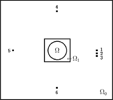
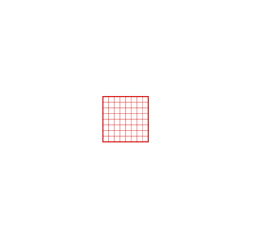
Figure 1: The schematic diagrams of inverse problem domain and light source locations. (a) Illustrates a layout of the inverse problem setting in 2-D. The circular disk $\Omega$ corresponds to a horizontal cross-section of the hemisphere part of phantom (the supposed “mouse head” in animal experiments), The computational domain $\Omega_{1}$ is a rectangle containing $\Omega$ inside, 6 light sources are located outside of the computational domain. Because of limitations of our device, we use only three locations of the light source along one line (number 1,2,3) to model the source $\mathbf{x}_{0}$ running along the straight line $L$. Light sources numbered 1,4,5,and 6 are used to construct an approximation for the tail function. (b) Depicts the computational domain $\Omega_{1}=\{(x,z),|x|<5.83,|z|<5.83\}$ (unit:mm) and its rectangular meshes for tail functions and inverse calculations for the numerical method of this paper. Actual mesh is much dense than these displayed. The diagram is not scaled to actual sizes.

We display in Fig. 1 the boundary data collection scheme in our experiment. We have used six locations of the light sources, see Fig. 1. Sources number 1,2 and 3 are the ones which model the source $\mathbf{x}_{0}$ running along the straight line $L,$ see (4). The distance between these sources was six (6) millimeters. Each light source means drilling a small hole in the phantom to fix the source position. It was impossible to place more sources in a phantom of this size that mimics actual mouse head. So, since the data for the functions $q_{n}$ are obtained via the differentiation with respect to the source position, we have used only two functions $q_{1},q_{2}$. Fortunately, the latter was sufficient for our goal of imaging of abnormalities. Sources 1,4,5,6 (Fig. 1) were used to approximate the tail function as described below. We construct that approximation in the domain $\Omega_{1}$ depicted on Fig. 1. This domain is (units in millimeters)

$$\Omega_{1}:=\left\{\mathbf{x}=\left(x,z\right):x_{1}=-5.83<x<x_{2}=5.83,z_{1}=-5.83<z<z_{2}=5.83\right\}.$$ (43)

5.2.1 The first stage of approximating the tail

Since this stage essentially relies on positions of sources 1,4,5,6, it makes sense to describe this stage in detail here, although it was also described in [17]. The light sources are placed as far as possible from the domain $\Omega_{1}$, so that the asymptotic approximations (45), (46) of solutions are applicable. Let $\mathbf{s}^{\left(j\right)}$ be the two-dimensional vector characterizing the position of the light source number $j$. First, consider the light source number 1. Denote

$$S^{\left(1\right)}:=S^{\left(1\right)}\left(x,z,\mathbf{s}^{\left(1\right)}\right)=\left|\left(x,z\right)-\mathbf{s}^{\left(1\right)}\right|.$$ (44)

Using (5), Theorem 2.1 and Lemma 2.4, we obtain for the function $\widetilde{w}=\ln u$

$$\widetilde{w}\left(x,z,\mathbf{s}^{\left(1\right)}\right)=-kS^{\left(1\right)}-\ln\left(2\sqrt{2\pi}\right)-\frac{1}{2}\ln S^{\left(1\right)}+p_{\infty}\left(x,z\right)+O\left(\frac{1}{S^{\left(1\right)}}\right),S^{\left(1\right)}\rightarrow\infty.$$ (45)

Since by (43) $\widetilde{w}\left(x,z_{1},\mathbf{s}^{\left(1\right)}\right)=\varphi\left(\mathbf{x,s}^{\left(1\right)}\right),\mathbf{x}\in\partial\Omega\cap\left\{z=z_{1}\right\},$ we use (45) to approximate the unknown function $p_{\infty}\left(x,z_{1}\right)$ as

$$p_{\infty}\left(x,z_{1}\right)=\widetilde{w}\left(x,z_{1},\mathbf{s}^{(1)}\right)+kS\left(x,z_{1},\mathbf{s}^{(1)}\right)+\frac{1}{2}\ln\left(\frac{\pi}{2S\left(x,z_{1},\mathbf{s}^{(1)}\right)}\right).$$ (46)

Formula (46) gives the value of $p_{\infty}\left(x,z_{1}\right)$ only at $z=z_{1}$. Since $\Omega_{1}$ is a square, we set the first guess for the tail as the one which is obtained from (46) by simply extending the values at $z=z_{1}$ to the entire domain of $\Omega_{1},$

$$\widetilde{w}\left(x,z,\mathbf{s}^{\left(1\right)}\right)=-kS^{\left(1\right)}\left(x,z,\mathbf{s}^{\left(1\right)}\right)-\ln\left(2\sqrt{2\pi}\right)-\frac{1}{2}\ln S^{\left(1\right)}\left(x,z,\mathbf{s}^{\left(1\right)}\right)+p_{\infty}\left(x,z_{1}\right),$$

where the function $S\left(x,z,\mathbf{s}^{\left(1\right)}\right)$ is given in (44). Next, we compute the function $u\left(x,z,\mathbf{s}^{\left(1\right)}\right)=\exp\left(\widetilde{w}\left(x,z,\mathbf{s}^{\left(1\right)}\right)\right)$ and get $a^{\left(1\right)}\left(x,z\right),\left(x,z\right)\in\Omega$ via (41), (42).

For light sources 4-6, we repeat the above procedure to get $a^{\left(4\right)}\left(x,z\right),a^{\left(5\right)}\left(x,z\right)$ and $a^{\left(6\right)}\left(x,z\right)$ respectively. Then we consider the average coefficient $\overline{a}(x,z)$ and set (see (42))

$$a\left(x,z\right):=\max(\overline{a}(x,z),k^{2}).$$ (47)

Next, we solve the forward problem (1), (2) for the light $\mathbf{s}^{\left(3\right)}$ with this coefficient $a\left(x,z\right)$ again to get $u\left(x,z,\overline{s}\right),\overline{s}=\left|\mathbf{s}^{\left(3\right)}\right|.$ The final approximate tail function obtained on the first stage is

$$T_{1}\left(x,z\right)=\frac{\ln u\left(x,z,\overline{s}\right)}{\overline{s}^{2}}.$$ (48)

5.2.2 The second stage for the tail

The second stage involves an iterative process that enhances the first approximation for the tail (48). We describe this stage only briefly here referring to [17] for details. In this case we use only one source number 3, $\mathbf{s}^{\left(3\right)}.$ Recall that $\left|\mathbf{s}^{\left(3\right)}\right|=\overline{s}$. Let the function $a\left(x,z\right)$ be the one calculated in (47). Denote $a_{1}\left(\mathbf{x}\right):=a\left(x,z\right).$ Next, we solve the following boundary value problem

$$\Delta u_{1}-a_{1}\left(\mathbf{x}\right)u_{1} = 0,\mathbf{x}\in\Omega_{1},$$

$$u_{1}|_{\partial\Omega_{1}} = \varphi\left(\mathbf{x},\overline{s}\right),\mathbf{x}\in\partial\Omega_{1}.$$

Then, we iteratively solve the following boundary value problems

$$\Delta w_{m}-a_{m}\left(\mathbf{x}\right)w_{m} = \left[a_{m}\left(\mathbf{x}\right)-a_{m-1}\left(\mathbf{x}\right)\right]u_{m-1},\text{ }m\geq 2,$$

$$w_{m}|_{\partial\Omega_{1}} = 0.$$

We set $u_{m}:=u_{m-1}+w_{m}.$ Next, using (41) and (42) with $u:=u_{m},$ we find the function $a_{m+1}\left(\mathbf{x}\right).$ We have computationally observed that this iterative process provides a convergent sequence $\left\{a_{m}\left(\mathbf{x}\right)\right\}$ in $L_{2}\left(\Omega_{1}\right).$ We stop iterations at $m:=m_{1}$, where $m_{1}$ is defined via

$$\frac{\left\|a_{m_{1}}-a_{m_{1}-1}\right\|_{L_{2}\left(\Omega_{1}\right)}}{\left\|a_{m_{1}-1}\right\|_{L_{2}\left(\Omega_{1}\right)}}\leq\varepsilon,$$ (49)

where $\varepsilon>0$ is a small number of our choice, and the norm in $L_{2}\left(\Omega_{1}\right)$ is understood in the discrete sense. Next, assuming that $u_{m_{1}}>0$, we set for the tail

$$T\left(\mathbf{x}\right)=\frac{1}{\overline{s}^{2}}\ln u_{m_{1}}\left(\mathbf{x}\right).$$ (50)

Then, using (50), we proceed with calculating of functions $q_{n}$ as described above.

6 Real Data

We now describe our experimental setup for collecting the optical tomography data from an optical phantom. This phantom is a man-made subject that has the same optical property as small animals. Such a phantom is a well-accepted standard to test reconstruction methods for real applications before animal experiments.

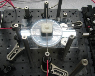
Figure 2: A photograph of the experimental setup. An optical phantom is connected with 4 laser fibers, the one on the right hand side is movable to locations 1,2, and 3 (Fig. 1). The gelatin made phantom has the shape of the rectangular box with a hemisphere on its top surface. The hemisphere mimics the head of a mouse with a mask exposing the crown part of the mouse. A CCD camera mounted above the phantom (not shown) provides light intensity measurements of the top surface of the phantom.

Fig. 2 is a photograph of our measurement setup. The center of the picture is the phantom (rectangular box with a hemisphere on top surface) which, in particular, contains a hidden inclusion inside (not visible in this photo). The hemisphere mimics the mouse head in animal experiments of stroke studies, and hidden inclusions of ink-mix mimic blood clots. The four needles are laser fibers that provide light sources in our experiments. The fiber on the right hand side of Fig. 2 can be moved to three other positions which are source positions 1,2,3 on Fig. 1. Three other fibers represent positions 4,5,6 of the source on Fig. 1. A CCD camera is mounted directly above the setup (not shown in photo), and the camera focus is on the top surface of the phantom. CCD stands for Charge Coupled Device. CCD camera with its sensitivity and response range is commonly used for near infrared laser imaging of animals.

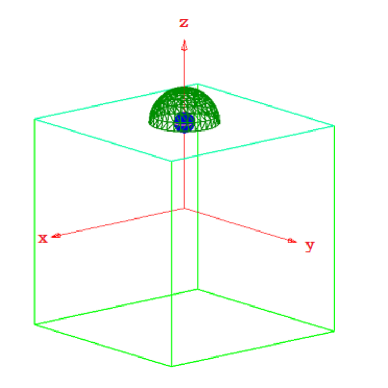
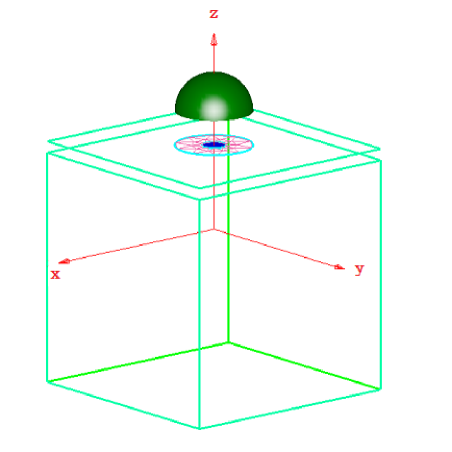
Figure 3: The schematic diagrams of our data acquisition process. (a) schematically depicts a 3-D phantom and its hidden inclusion (shown in meshed surface) 5mm below the phantom. The light source is placed at various locations on the top surface of the rectangular block (see Fig. 1) and light intensity measurements are taken on the top surface of phantom. (b) The measurement surface by a CCD camera. The data are collected from the surface of the hemisphere as well as from the un-shaded area of top rectangle, both area are lifted from the phantom in this drawing for a better illustrative purpose. The rectangular figure in Fig. 3 also illustrates the middle a 2-D cross-section (meshed circle) of the presumed “animal head”, at the boundary of which light intensity data are collected for the reconstruction. The light intensity at the 2-D cross-section (except for the boundary) is obstructed by the top surface of the hemisphere. Light sources are also located in the same plane as this cross-section area. The 2-D inverse problem is solved in this cross-section by ignoring the dependence on the orthogonal coordinate.

The purpose of this experimental setup is to study the feasibility of using our numerical method in an animal stroke model. In the case of a real animal, the top hemisphere (meshed shape in Fig. 6.2a) is to be replaced by a mouse head and the rectangular block of phantom to be replaced by an optical mask filled with a matching” fluid (a tissue-like solution with the optical properties similar to the animal skin/skull). The image reconstruction should provide the spatial distribution of the optical coefficient $a(\mathbf{x})$ (directly related to the blood content) in a 2-D cross-section of the animal brain.

The goal to is to accomplish a noninvasive imaging means to monitor and investigate hemodynamic dysfunction during ischemic stroke in animal models. The current experimental setup works only for small animals, such as rats, but not for human brains due to the limited penetration depth of NIR light through a larger size and thicker bone structure of the skull. The methodology developed here, however, may be applicable to a neonate head, while further studies are needed to confirm such an expectation.

Our inverse reconstruction is performed in the 2-D plane depicted in Fig. 3, with the optical parameter distribution of the medium inside the circle (at the center of Fig. 3) as an unknown coefficient in the photon diffusion model. Should we need a diagnosis of a different cross-section of mouse brain in animal experiments, we need a different optical mask filled with matching fluid, and repeat both the experiment and the reconstruction.

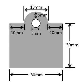
Figure 4: Dimensions of the phantom, shown in a vertical cross-section at the center of the phantom from side view. The circle in Fig. 1 corresponds to the boundary of the meshed circle in Fig. 3. This also corresponds to the boundary of the 13 mm diameter circle at a top view above the rectangular box (but not related to circle or semicircle in this graph). The 5 mm diameter hollow sphere is for the placement of inclusions, filled with liquids of different compositions to emulate strokes. The hidden inclusion is 5 mm below the top surface.

The geometry of the phantom (shown in a vertical central cross-section) is depicted in Fig. 4 with dimensions specified. The phantom is shaped by a hemisphere (diameter 13 mm) on the top of a cube of 30mm $\times$ 30mm $\times$ 30mm. A spherical hollow of 5 mm diameter is located inside the phantom, with its top 5mm below the top surface (Fig. 4). The location of this hollow is symmetric here but can be in any place when needed. One and two spherical hollows of 3mm diameter inside the phantom are also used in experiments (see Section 8 for detail). We fill the hollow with liquids made of different kinds of ink/intralipid mix to model strokes by blood clots. Intralipid is a product for fat emulsion, which mimics the response of human or animal tissue to light at wavelengths in the red and infrared ranges. The phantom is made of gelatin mixed with the intralipid. The percentage of intralipid content is adjustable. So that the phantom has the same optical parameters as the background medium of the target animal model. At the location of the inclusion (the hollow), we inject ink/intralipid mixed fluids whose optical absorption coefficients are 2 times, 3 times and 4 times higher than in the background. Also, we use the pure black ink to test our reconstruction method for the case of the infinite absorption. Different levels of the inclusion/background absorption ratio are used to validate our method for its ability for different blood clots. Light intensity measurements are taken directly above the semicircle in Fig. 4. We note that Fig. 1 shows a top view of the layout but Fig. 4 shows a cross-section from side view. The disk region $\Omega$ in Fig. 1 corresponds to the meshed area in Fig. 3 as well as a horizontal cross-section of the 13 mm hemisphere. The reason we use such a geometry is that we need to test our capability to reconstruct inclusions at several different depth (moving up and down vertically as in Fig. 4) as well as at different locations (moving horizontally in Fig. 3).

7 Processing Real Data

As it is typical when working with imaging from real data, we need to make several steps of data pre-processing before applying our inverse algorithm.

7.1 Computational domains

We need to use several computational domains. The computational domains and meshes used in our numerical calculation involve four domains. Fig. 5(a) - Fig. 5(c) and Fig. 1 are the finite element meshes on each of these domains $\Omega,\Omega_{0},\Omega_{0}\diagdown\Omega,\Omega_{1}$ respectively. In actual computations we use more refined meshes for each domain than those illustrated. Therefore, figures are not scaled to actual sizes.

(a) $\Omega$

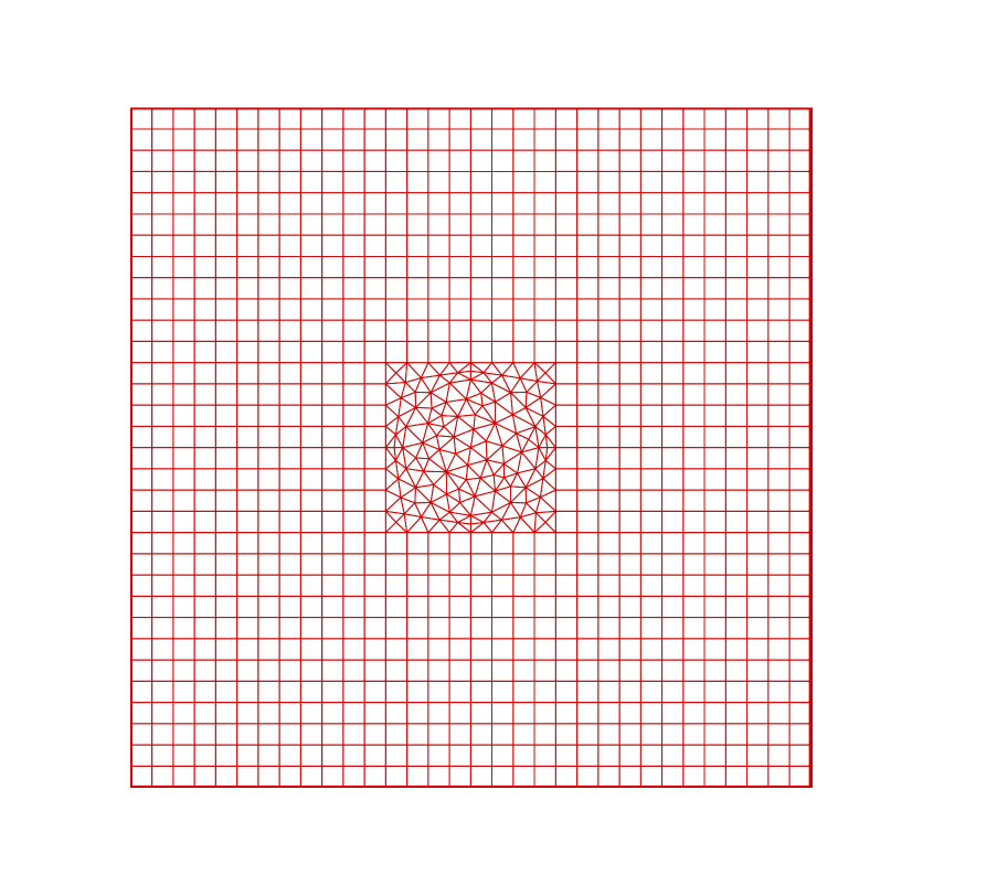
(b) $\Omega_{0}$

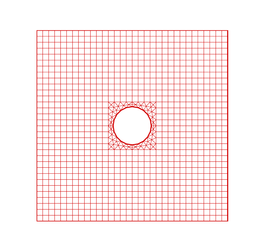
(c) $\Omega_{0}\backslash\Omega$

Figure 5: (a) The domain $\Omega=\{(x,z),\sqrt{x^{2}+z^{2}}<4.63\}$ (units: mm) with a triangular mesh. The domain represents a cross-section of our phantom, and the inclusion inside $\Omega$ is to be reconstructed. (b) The domain $\Omega_{0}=\{(x,z),|x|<23.32,|z|<23.32\}$ (units: mm). The domain $\Omega_{0}$ contains $\Omega$ and light sources. Meshed small square is the domain $\Omega_{1}$ which is the same as on Fig. 1. Computations of the inverse problem are performed in $\Omega_{1}.$ (c) Shows $\Omega_{0}\diagdown\Omega$ the domain used for data processing. To smooth out the measurement noise, equation (1) with the Dirichlet boundary conditions $u\mid_{\partial\Omega}=\varphi\left(x,x_{0}\right)$, $u\mid_{\partial\Omega_{0}}=0$ is solved in $\Omega_{0}\diagdown\Omega$. Then the smoothed data along $\partial\Omega_{1}$ is used for the inverse problem.

Here the disk $\Omega$ is the domain of interest that contains the inclusion, corresponding to the meshed area in Fig. 3. It reflects a cross-section of the hemisphere of phantom in Fig. 3. The light intensity data used in our computations are originated by the measurements at $\partial\Omega$ by taking pictures with CCD camera on the top of phantom as discussed, shown in Fig. 3. The CCD camera collected data is acquired from the surface of the hemisphere and the un-shaded area of the top rectangle, and we extract only the needed data for $\partial\Omega$ i.e., the circle in Fig. 3 by getting the data at these locations as boundary values. Here $\Omega=\left\{\left(x,z\right)|\sqrt{x^{2}+z^{2}}\leq 4.63mm\right\}$.

On Fig. 5 $\Omega_{0}$ is a large domain, which can be interpreted as a truncated plane $\mathbb{R}^{2}.$ Indeed, one cannot practically solve the forward problem (1), (2) in the infinite plane $\mathbb{R}^{2}.$ Light sources are located in $\Omega_{0}\diagdown\Omega$. The background simulation and calibration of background parameters are performed in $\Omega_{0}.$ To smooth out the noise in the data, equation (1) is solved in $\Omega_{0}\diagdown\Omega$ for each source position, which is similar with [24]. Because of (3), we use $a\left(\mathbf{x}\right):=k^{2}$ for $x\in\Omega_{0}\diagdown\Omega.$ In this procedure the Dirichlet boundary condition at $\partial\Omega$ is taken from the real data, and we use the zero Dirichlet boundary condition at $\partial\Omega_{0}.$ As a result, we obtain the smoothed Dirichlet boundary condition at $\partial\Omega_{1}$ for each source location. We solve the inverse problem in $\Omega_{1},$ and $\Omega\subset\Omega_{1}$.

7.2 Data pre-processing and approximations of boundary conditions

As it was stated in subsection 7.1, to smooth out our measurement data, we solve the Dirichlet boundary problem for equation (1) with $a\left(\mathbf{x}\right)\equiv k^{2}$ for $\mathbf{x}\in\Omega_{0}\diagdown\Omega$ (Fig. 5(c)) for each source location. Namely,

$$\Delta u-k^{2}u = -\delta\left(\mathbf{x}-\mathbf{s}^{\left(i\right)}\right),\mathbf{x}\in\Omega_{0}\diagdown\Omega,$$ (51)

$$u\mid_{\partial\Omega} = \varphi\left(\mathbf{x},\mathbf{s}^{\left(i\right)}\right),\text{ }u\mid_{\partial\Omega_{0}}=0.$$

Here $k^{2}=3\mu_{s}^{\prime}\mu_{a}$ is the background value and $\varphi\left(\mathbf{x,}\mathbf{s}^{\left(i\right)}\right)$ is the experimentally measured data for the light source $\mathbf{s}^{\left(i\right)}$. Let $\overline{\varphi}\left(\mathbf{x},\mathbf{s}^{\left(i\right)}\right)$ be the trace of the solution of the Dirichlet boundary value problem (51) at $\mathbf{x}\in\partial\Omega_{1}$. We solve the inverse problem in the square $\Omega_{1}$ with the smoothed data $u\mid_{\partial\Omega_{1}}=\overline{\varphi}\left(\mathbf{x},\mathbf{s}^{\left(i\right)}\right).$ We have shown in [25, 27] that solving inverse problems in the original domain $\Omega$ and extended domain $\Omega_{1}$ are equivalent mathematically. But numerically the noisy component in $\overline{\varphi}\left(\mathbf{x},\mathbf{s}^{\left(i\right)}\right)$ is much smaller than in $\varphi\left(\mathbf{x},\mathbf{s}^{\left(i\right)}\right).$ This smoothing effect takes place because the inverse problem is solved in $\Omega_{1}$.

7.3 The forward problem and calibration

We now address the question on which value of $k^{2}$ one should use when working with the real data. The optical properties of the background of the phantom (without the hidden inclusion) are known theoretically from the concentration of intralipid in the mix. However, there is a discrepancy between the theoretical value and actual measurements. Before we solve the inverse problem to image hidden inclusions, we calibrate our model by adjusting the background value of $k^{2}$ to the real data measured for the reference medium, which is the phantom without inclusion, i.e. the hollow is filled with the same intralipid solution as that in the phantom itself.

First, we numerically solve the forward problem with the source position $\mathbf{s}^{\left(1\right)}$ in the domain $\Omega_{0}$ without any inclusion,

$$\Delta u-k^{2}u = -A\delta\left(\mathbf{x}-\mathbf{s}^{\left(1\right)}\right),\mathbf{x}\in\Omega_{0},$$ (52)

$$u\mid_{\partial\Omega_{0}} = 0,$$

where $k^{2}=3\mu_{s}^{\prime}\mu_{a}$ is the background value. Then we calibrate the parameter $\mu_{a}$ (fixing $\mu_{s}^{\prime}$) as well as the amplitude $A>0$ of light source in our model (52) to match the measured light intensity for $\mathbf{s}^{\left(1\right)}$ for the uniform background. We do not know the number $A$. Thus, we choose $A$ in such a way that $u_{comp}\left(\mathbf{x}_{\max},\mathbf{s}^{\left(1\right)}\right)\approx u_{meas}\left(\mathbf{x}_{\max},\mathbf{s}^{\left(1\right)}\right).$ Here $\mathbf{x}_{\max}$ is the brightest point, i.e. the far right point on $\partial\Omega$, being closest to the light source. Also, $u_{comp}\left(\mathbf{x}_{\max},\mathbf{s}^{\left(1\right)}\right)$ and $u_{meas}\left(\mathbf{x}_{\max},\mathbf{s}^{\left(1\right)}\right)$ are computed and measured light intensities respectively. Next, we should approximate the constant $k^{2}.$ To do this, we take another sampling point $\mathbf{x}_{\min}$ with the minimal light intensity, which is the farthest left point on $\partial\Omega$. Next we consider ratios $R_{comp}\left(k^{2}\right),R_{meas},$ where

$$R_{comp}\left(k^{2}\right)=\frac{u_{comp}\left(\mathbf{x}_{\max},\mathbf{s}^{\left(1\right)}\right)}{u_{comp}\left(\mathbf{x}_{\min},\mathbf{s}^{\left(1\right)}\right)},\text{ }R_{meas}=\frac{u_{meas}\left(\mathbf{x}_{\max},\mathbf{s}^{\left(1\right)}\right)}{u_{meas}\left(\mathbf{x}_{\min},\mathbf{s}^{\left(1\right)}\right)}.$$

These ratios are independent on the number $A$ in (52). We choose $k^{2}$ such that $R_{comp}\left(k^{2}\right)\approx R_{meas}.$ As a result, the calibrated value of $k^{2}$ was $k^{2}=2.403.$ This computed value matches quite well the theoretical value of 2.4 of the intralipid solution we have used.

8 Results Of the Reconstruction

Let $a_{incl}=a\left(\mathbf{x}\right)$ be the value of $a\left(\mathbf{x}\right)$ inside the inclusion and $a_{b}=k^{2}=2.403$ be the value of the coefficient $a\left(\mathbf{x}\right)$ in the background, which was computed in subsection 7.3. Our ratios $a_{incl}/a_{b}$ where

$$\frac{a_{incl}}{a_{b}}=2,3,4,\infty.$$ (53)

The value $a_{incl}/a_{b}=\infty$ means that the inclusion was filled with a black absorber, i.e. black ink. Table 1 gives a detailed information of our real data with different positions, numbers, diameters and contrast of inclusions. ”Y” means that the experiment was done for this setting, and ”-” means that the experiment was not done. Note that in Group 3 we have imaged two different inclusions simultaneously.

Inclusion Groups	Positions	Diameters	Ratio2	Ratio3	Ratio4	Ratio$\infty$
Group 1		5mm	Y	Y	Y	Y
Group 2		3mm	Y	Y	Y	-
Group 3		3mm	Y	Y	Y	-

Table 1: Real data

As described in sub-subsection 5.2.1, we construct the “asymptotic tail” on the first stage using light sources 1,4,5, and 6 as an initial approximation, to be followed by other subroutines for further refinements. The image of the function $a(x,z)$ in (47) is depicted on Fig. 6, for a phantom where the theoretical value of the inclusion/background contrast (53) was $a_{incl}/a_{b}=3$. Images from the asymptotic tails for other phantoms listed in Table 8.1 were similar.

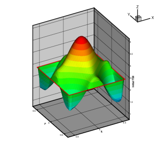
Figure 6: The function $a\left(x,z\right)$ in (47) is depicted. This function was obtained on the first stage procedure for the tail (sub-subsection 5.2.1) as an initial approximation. The initial reconstruction is obtained from a phantom where the theoretical value of the inclusion/background contrast (53) was $a_{incl}/a_{b}=3.$

Figures 7- Fig. 9 depict the reconstructed images from our real data. Fig. 7 depicts the 3D plots of reconstructed images of group 1 for contrast values of: 2:1, 3:1, 4:1 and $\infty:1$, from the left to the right respectively. Fig. 8 - Fig. 9 show 2:1, 3:1, 4:1, from left to right respectively for groups 2,3. In all our examples $\varepsilon=10^{-5}$ in (49). The finally reconstructed results for contrasts $a_{b}^{-1}\max a\left(\mathbf{x}\right)$ are listed in Table 2. Note that our above reconstruction algorithm does not use any knowledge of neither the location of the inclusion, nor the contrast value $a_{incl}/a_{b}$.

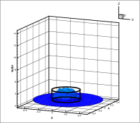
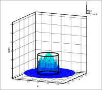
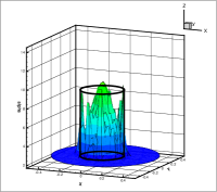
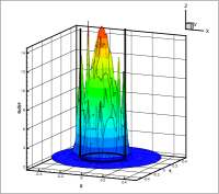
Figure 7: Reconstructed inclusion contrast of data group 1, actual contrasts are 2:1, 3:1, 4:1 and $\infty:1$, from left to right respectively. The transparent frames show the theoretical values of inclusion/background contrasts of actual inclusions, which are made of different ink-intralipid mix.

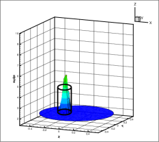
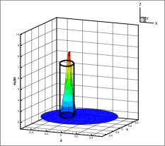
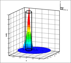
Figure 8: Reconstructed inclusion contrast of data group 2, actual contrasts are 2:1, 3:1, 4:1, from left to right respectively. The transparent frames show the theoretical values of inclusion/background contrasts of actual inclusions, which are made of different ink-intralipid mix.

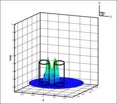
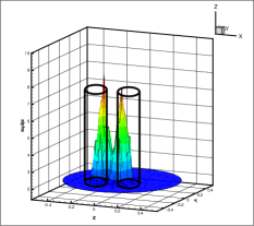
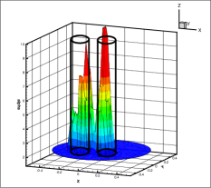
Figure 9: Reconstructed inclusion contrast of data group 3, actual contrasts are 2:1, 3:1, 4:1, from left to right respectively. The transparent frames show the theoretical values of inclusion/background contrasts of actual inclusions, which are made of different ink-intralipid mix.

	The true contrast $a_{incl}/a_{b}$	$a_{b}^{-1}\max a\left(\mathbf{x}\right)$	Relative Error
Group 1	2	2.11	0.056
	3	2.9	0.032
	4	4.22	0.057
	$\infty$	6.69	unknown
Group 2	2	2.33	0.167
	3	3.29	0.0986
	4	4.57	0.143
Group 3	2	2.29	0.148
	3	3.49	0.164
	4	4.58	0.147

Table 2: Reconstructed values of the contrast $a_{b}^{-1}\max a\left(\mathbf{x}\right)$ within imaged inclusions and they relative errors, $a_{b}=2.403,$ compare with (8.1).

9 Summary

We have worked with a set of real data, using the approximately globally convergent numerical method of [17] for a Coefficient Inverse Problem for an elliptic equation. These data mimic imaging of clots in the heads of a mouse. We have introduced a new concept of the approximate global convergence property and have established this property for the discrete case of a finite number of finite elements, unlike the continuous case of [17]. Figures 7- Fig. 9 as well as Table 2 demonstrate that our are quite accurate, including both inclusion/background contrasts and locations of inclusions. Note that accurate values of contrasts are usually hard to reconstruct via locally convergent algorithms. On the other hand, these values are especially important for our target application, since they might be used for monitoring stroke treatments. Therefore, following the concept of Steps 1-6 of subsection 4.1, we conclude that our approximate mathematical model of subsection 4.3 is a valid one.

Acknowledgments

The work of all authors was supported by the National Institutes of Health grant number 1R21NS052850-01A1. In addition, the work of MVK was supported by the U.S. Army Research Laboratory and U.S. Army Research Office under the grant number W911NF-11-1-0399.

References

- [1] M. Abramowitz and A. Stegun, Handbook of Mathematical Functions (Washington, DC: National Bureau of Standards), 1964.
- [2] N.V. Alexeenko, V.A. Burov and O.D. Rumyantseva, Solution of a three-dimensional acoustical inverse scattering problem: II. Modified Novikov algorithm, Acoust. Phys., 54, 407-419, 2008.
- [3] R.R. Alfano, R.R. Pradhan and G.C. Tang, Optical spectroscopic diagnosis of cancer and normal breast tissues, J. Opt. Soc. Am. B, 6, 1015-1023, 1989.
- [4] S. Arridge, Optical tomography in medical imaging, Inverse Problems, 15, 841-893, 1999.
- [5] A.B. Bakushinskii and M.Yu. Kokurin, Iterative Methods for Approximate Solutions of Inverse Problems, Springer, New York, 2004.
- [6] L. Beilina and M.V. Klibanov, A globally convergent numerical method for a coefficient inverse problem, SIAM J. Sci. Comp., 30, 478-509, 2008.
- [7] L. Beilina and M.V. Klibanov, A posteriori error estimates for the adaptivity technique for the Tikhonov functional and global convergence for a coefficient inverse problem, Inverse Problems, 26, 045012, 2010.
- [8] L. Beilina and M.V. Klibanov, Reconstruction of dielectrics from experimental data via a hybrid globally convergent/adaptive inverse algorithm, Inverse Problems, 26, 125009, 2010.
- [9] L. Beilina and M.V. Klibanov, Approximate Global Convergence and Adaptivity for Coefficient Inverse Problems, Springer, New York, 2012.
- [10] M. Born and E. Wolf, Principles of Optics: Electromagnetic Theory of Propagation, Interference and Diffraction of Light, Cambridge University Press, 1970.
- [11] V.A. Burov, S.A. Morozov and O.D. Rumyantseva, Reconstruction of fine-scale structure of acoustical scatterers on large scale contrast background, Acoust. Imaging, 26, 231-238, 2002.
- [12] P.G. Ciarlet, The Finite Element Method for Elliptic Problems, SIAM, Philadelphia, 2002.
- [13] H.W. Engl, M. Hanke and A. Neubauer, Regularization of Inverse Problems, Kluwer Academic Publishers, Boston, 2000.
- [14] D. Gilbarg and N.S. Trudinger, Elliptic Partial Differential Equations Of the Second Order, Springer-Verlag, New York, 1983.
- [15] D. Isaacson, J.L. Mueller, J.C. Newell and S. Siltanen, Reconstructions of chest phantoms by the D-bar method for electrical impedance tomography, IEEE Trans. Med. Imaging, 23, 821-828, 2004.
- [16] S. I Kabanikhin and M.A. Shishlenin, Numerical algorithm for two-dimensional inverse acoustic problem based on Gel’fand-Levitan-Krein equation, J. Inverse and Ill-Posed Problems, 18, 979-995, 2011.
- [17] M.V. Klibanov, J. Su, N. Pantong, H. Shan and H. Liu, A globally convergent numerical method for an inverse elliptic problem of optical tomography, Applicable Analysis, 89, 861-891, 2010.
- [18] M.V. Klibanov, M.A. Fiddy, L. Beilina, N. Pantong and J. Schenk, Picosecond scale experimental verification of a globally convergent numerical method for a coefficient inverse problem, Inverse Problems, 26, 045003, 2010.
- [19] A.V. Kuzhuget, L.Beilina and M.V. Klibanov, Approximate global convergence and quasi-reversibility for a coefficient inverse problem with backscattering data, Journal of Mathematical Sciences, 181, 126-163, 2012.
- [20] A.V. Kuzhuget, L. Beilina, M.V. Klibanov, A. Sullivan, L. Nguyen and M.A. Fiddy, Blind backscattering experimental data collected in the field and an approximately globally convergent inverse algorithm, Inverse Problems, 28, 095007, 2012.
- [21] J. Mueller and S. Siltaren, Direct reconstruction of conductivities from boundary measurements, SIAM J. Sci. Comp., 24, 1232-1266, 2003.
- [22] R.G. Novikov, The bar approach to approximate inverse scattering at fixed energy in three dimensions, Int. Math. Res. Reports, 6, 287-349, 2005.
- [23] R.G. Novikov and M. Santacesaria, Monochromatic reconstruction algorithms for two-dimensional multi-channel inverse problems, International Mathematics Research Notices, to appear.
- [24] N. Pantong, J. Su, H. Shan, M.V. Klibanov and H. Liu, A globally accelerated reconstruction algorithm for diffusion tomography with continuous-wave source in arbitrary convex shape domain, Journal of the Optical Society of America, A, 26, 456-472, 2009.
- [25] H. Shan, M.V. Klibanov, J. Su, N. Pantong and H. Liu, A globally accelerated numerical method for optical tomography with continuous wave source, J. Inverse and Ill-Posed Problems, 16, 765-792, 2008.
- [26] J. Su, H. Shan, H. Liu and M.V. Klibanov, Reconstruction method from a multiplesite continuous-wave source for three-dimensional optical tomography, J. Optical Society of America A, 23, 2388-2395, 2006.
- [27] A.N. Tikhonov, A.V. Goncharsky, V.V. Stepanov and A.G. Yagola, Numerical Methods for Solutions of Ill-Posed Problems, Kluwer, London, 1995.