FUV and X-ray irradiated protoplanetary disks: a grid of models

Abstract

Context. Planets are thought to eventually form from the mostly gaseous ($\sim 99\%$ of the mass) disks around young stars. The density structure and chemical composition of protoplanetary disks are affected by the incident radiation field at optical, far-ultraviolet (FUV), and X-ray wavelengths, as well as by the dust properties.

Aims. The effect of FUV and X-rays on the disk structure and the gas chemical composition are investigated. This work forms the basis of a second paper, which discusses the impact on diagnostic lines of, e.g., C⁺, O, H₂O, and Ne⁺ observed with facilities such as Spitzer and Herschel.

Methods. A grid of 240 models is computed in which the X-ray and FUV luminosity, minimum grain size, dust size distribution, and surface density distribution are varied in a systematic way. The hydrostatic structure and the thermo-chemical structure are calculated using Protoplanetary Disk Model (ProDiMo), with the recent addition of X-rays.

Results. The abundance structure of neutral oxygen is very stable to changes in the X-ray and FUV luminosity, and the emission lines will thus be useful tracers of the disk mass and temperature. The C⁺ abundance distribution is sensitive to both X-rays and FUV. The radial column density profile shows two peaks, one at the inner rim and a second one at a radius $r=5-10$ AU. Ne⁺ and other heavy elements have a very strong response to X-rays, and the column density in the inner disk increases by two orders of magnitude from the lowest ($L_{\rm X}=10^{29}$ erg s^-1) to the highest considered X-ray flux ($L_{\rm X}=10^{32}$ erg s^-1). FUV confines the Ne⁺ ionized region to areas closer to the star at low X-ray luminosities ($L_{X}=10^{29}$ erg s^-1). H₂O abundances are enhanced by X-rays due to higher temperatures in the inner disk than in the FUV only case, thus leading to a more efficient neutral-neutral formation channel. Also, the higher ionization fraction provides an ion-molecule route in the outer disk. The line fluxes and profiles are affected by the effects on these species, thus providing diagnostic value in the study of FUV and X-ray irradiated disks around T Tauri stars.

1 Introduction

New observing facilities in the past decade pushed our understanding of protoplanetary disks from a rough picture of a vertically layered structure to a wealth of details on the composition and two-dimensional structure of the gas and dust of these disks. In the infrared, the Spitzer Space Telescope performed systematic studies of nearby star-forming regions. The spectral energy distributions (SEDs) revealed the physical structure of disks, e.g., the presence of gaps, source-to-source variations and important statistics on SED types, which allow evolutionary scenarios to be built (cf. Merín et al., 2010). Extensive gas-phase emission line studies with Spitzer provide a first indication of chemical diversity across stellar spectral types (cf. Najita et al., 2009; Pontoppidan et al., 2010; Lahuis et al., 2007). In the near-infared, there have been large ground-based studies with, e.g., the VLT and the Keck telescope resolving the lines to study the kinematics (spatial origin of the lines in hot disk surfaces and winds) and their excitation mechanisms (thermal and fluorescence; Brittain et al., 2010; Pontoppidan et al., 2011; Fedele et al., 2011). In the past two years, the Herschel Space Observatory extended the spectral window to the far-IR and submm, with spectral line scans within the Dust, Ice, and Gas in Time (DIGIT) key program (PI: N. Evans) for many Herbig disks, e.g., HD 100549 (Sturm et al., 2010), water studies of a few selected targets, such as TW Hya (Hogerheijde et al., 2011) from the Water in Star-forming Regions with Herschel (WISH) key program (PI: E.van Dishoeck), and large statistical gas surveys targeting the dominant cooling lines (e.g., Mathews et al., 2010; Meeus et al., 2012; Dent & the GASPS team, 2012; Riviere-Marichalar et al., 2012) in the Gas in Protoplanetary Systems (GASPS) key program (PI: B. Dent). The HIFI and some PACS line detections deal with the cold water, while the 63.3 $\mu$m H₂O line possibly probes the inner water reservoir.

Observational studies report trends in emission line strength with the irradiation of the central star. Güdel et al. (2010) find that the [Ne ii] emission at 12.81 $\mu$m correlates with the X-ray luminosity of the central star; the slope of the correlation for nonjet sources is $0.44\pm 0.18$. Pinte et al. (2010) and Meeus et al. (2012) show that the [O i] 63 $\mu$m line flux increases with stellar luminosity and that this is largely driven by the strength of the far-ultraviolet (FUV) luminosity. Riviere-Marichalar et al. (2012) report a tentative trend of the 63.3 $\mu$m water line flux with X-ray luminosity.

It is obvious from previous works that the most relevant parameter for the SED is the total stellar luminosity; in most cases, $L_{\rm X}$ and $L_{\rm FUV}$ present only a small fraction of this and hence by themselves do not cause significant SED changes. However, recent near-IR high-contrast imaging with HiCIAO on the Subaru 8.2 m telescope allowed probing of the inner disk structure on scales below 0.1″ (Thalmann et al., 2010; Hashimoto et al., 2011). This offers the possibility of a direct probe, e.g., the height of the inner rim as predicted by protoplanetary disk models. Thi et al. (2011) predicted that the height of the inner rim could be a factor two higher when the vertical hydrostatic structure takes into account the gas temperature at the inner rim. Aresu et al. (2011) show that the height of the inner rim increases in disk models with the impinging stellar $L_{\rm X}$.

In the last decade, much theoretical progress has taken place to support the interpretation of the wealth of new observations, specifically the gas observations. The foundation was laid by Chiang & Goldreich (1997), D’Alessio et al. (1998), and Dullemond et al. (2001), whose layered dust disk models have helped to interpret SEDs for irradiated disks (see Dullemond et al. 2007 for a review of disk structure models). Based on this, several groups focussed on the effects of FUV and X-rays on the thermal and chemical structure of the gas in a pre-prescribed protoplanetary disk model, e.g., van Zadelhoff et al. (2003), Kamp & Dullemond (2004), Jonkheid et al. (2004), and Glassgold et al. (2004). In a subsequent step, Nomura & Millar (2005), Gorti & Hollenbach (2008), and Woitke et al. (2009) studied the chemical structure of disks, while self-consistently solving for the vertical hydrostatic equilibrium using the gas temperature. Most recently, Aresu et al. (2011) performed an exploratory study to assess the relative importance of FUV and X-rays by expanding the existing Protoplanetary Disk Model (ProDiMo) code to include X-ray processes. The modeling efforts that solve for the vertical disk structure are computationally expensive because the chemical networks, heating/cooling balance, 2D continuum radiative transfer, and hydrostatic equilibrium have to be solved iteratively. Hence, these studies have largely focussed on a single representative disk model, or at most a handful of models varying one specific parameter. However, large-model grids are in principle required to understand the potential diagnostic power of certain observables. So far examples for this are large grids (of the order of 200 000-300 000 models) of parametrized dust disk models to study SED diagnostics (Robitaille et al., 2006) and of parametrized gas/dust disks to study the gas emission line diagnostics (Woitke et al., 2011; Kamp et al., 2011).

In this paper, we perform for the first time an extensive analysis of a grid of 240 self-consistent disk models (including the vertical disk structure) to study the effects of X-rays, FUV, and the relative importance of grain size and gas surface density distribution on the thermal, chemical, and physical structure of disks around T Tauri stars. This paper builds on the implementation of X-rays into the ProDiMo code as described in Aresu et al. (2011). While we discuss here foremost the physical and chemical structure of the models and how they change with irradiation, a companion paper (Aresu et al., 2012, paper II), discusses the power of line diagnostic in disentangling these effects. The paper is structured in the following way: Sect. 2 describes the updates on the code and the range of parameters used in the grid. The effects on disk temperature and density structure will be discussed in Sect. 3. The resulting distribution of various key species and its key reactions are extensively described in Sect. 4. Sect. 5 shows the radial column density distributions. Those are key in understanding the line profiles, which is the topic of the accompanying paper II. Sect. 6 summarizes the conclusions and implications of the paper.

2 Updates on ProDiMo and the calculated grid

The original ProDiMo code (Woitke et al., 2009) is based on the code as discussed by Kamp & Dullemond (2004). The original model includes (1) frequency-dependent two-dimensional dust continuum radiative transfer, (2) kinetic gas-phase and FUV photo-chemistry, (3) ice formation, and (4) detailed non-local thermodynamic equilibrium (non-LTE) heating and cooling with (5) a consistent calculation of the hydrostatic disk structure. The models are characterized by a high degree of consistency among the various physical, chemical, and radiative processes, since the mutual feedbacks are solved iteratively. Aresu et al. (2011) included X-ray heating and chemical processes, guided by work from Maloney et al. (1996), Glassgold et al. (2004), and Meijerink & Spaans (2005), while most recently the X-ray chemistry processes are updated following Ádámkovics et al. (2011). This includes an extension of our chemical network with species such as Ne, Ar, and their singly and doubly ionized states, as well as other heavy elements. We added Ne⁺, Ne²⁺, Ar⁺ and Ar²⁺ in the heating/cooling balance and also implemented an extended sulfur chemistry (following Leen & Graff, 1988; Meijerink et al., 2008, e.g., SO, SO₂, HS, and their related reactions were added) to achieve a proper calculation of the sulfur-based species abundances. This allowed us to make more realistic predictions of, e.g., the sulfur fine-structure lines. A detailed description on the treatment of X-ray chemistry in the code is given in Appendix A.

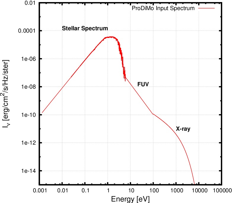
Figure 1: Input spectrum for model with $L_{\rm X}=10^{30}$ erg s^-1 and $L_{\rm FUV}=10^{31}$ erg s^-1.

Our input spectrum is composed of the stellar spectrum and a FUV excess as described in Woitke et al. (2009), along with an X-ray component as outlined in Aresu et al. (2011). The FUV excess (from 92.5 to 205 nm) spectrum is a power law with $I_{\nu}(\lambda)\propto\lambda^{1.2}$. The X-ray spectrum (0.1 - 10 keV) has been chosen following Glassgold et al. (2007) and is the same we used in Aresu et al. (2011). It is a bremsstrahlung spectrum with $I_{\nu}(E)\propto 1/E\times\exp(-E/kT)$ (see Fig. 1). We varied those quantities that could potentially affect the penetration of X-ray and FUV radiation and change the energy deposition through the disk. For example, we use two different values for the dust size distribution power law. The first value, generally used in the literature for the ISM, is a power law index of $a_{\rm pow}=3.5$. It is well known, though, that dust coagulation is the seed process that in timescales of a few million years leads to the formation of planetesimals. To model a disk that could have undergone dust coagulation, we also adopt a shallower power law index of $a_{\rm pow}=2.5$. For the same reason, we vary the minimum dust size: 0.1, 0.3, and 1 $\mu m$. These two parameters ($a_{\rm min}$ and $a_{\rm pow}$) determine the FUV opacity and, as a result, impact the amount of energy reprocessed by the photoelectric heating. Ultimately, the parameters affect the gas thermal balance in the disk. The changing opacity and optical depth also impact the dust temperature $T_{\rm dust}$.

Aresu et al. (2011) performed an exploratory study on the influence of X-rays and FUV irradiation on the structure of protoplanetary disks, for X-ray luminosities ranging from $L_{x}=10^{29}-10^{32}$ erg s^-1. The range of values for this particular parameter is based on the outcome of the Taurus survey (Güdel et al., 2007), which showed that X-ray-active T Tauri stars emit in the range $L_{\rm X}=10^{29}-10^{31}$ erg s^-1. The model with $L_{X}=10^{32}$ erg s^-1, on the other hand, is an extreme case with interesting implications in terms of modeling. FUV excess emission from classic T Tauri stars between 6 and 13.6 eV is believed to arise from accretion spots on the surface of the star and stellar activity. The disk is truncated to several stellar radii from the star magnetic field, which channels matter toward the stellar photosphere. Shocks in the outer layers of the star cause the temperature to rise and emit FUV photons, which results in a FUV excess with respect to the stellar luminosity in the same band (Gullbring et al., 2000). Gorti & Hollenbach (2008) infer the FUV excess luminosity (91.2 nm $<h\nu<$ 205 nm) to be between $L_{\rm FUV}/L_{*}\sim 10^{-2}-10^{-3}$ . In our grid, we decided to scale the FUV flux so that we obtain the same range of luminosities as we use for the X-rays. The adopted values of $L_{\rm FUV}/L_{\rm*}$ are then 2.6$\times 10^{-2}$, 2.6$\times 10^{-3}$, 2.6$\times 10^{-4}$, and 2.6$\times 10^{-5}$. This way we can directly compare the input energy radiation in the FUV and X-ray band as well as its effects on the disk. We also explore two different values for the surface density power law distribution $\epsilon$, which is defined as $\Sigma(r)=\Sigma(r_{0})\times(r/r_{0})^{-\epsilon}$: Hayashi (1981) derived the value $\epsilon=1.5$ in his model for the minimum mass solar nebular (MMSN) and their diagnostic value for our own solar system, while Hartmann (1998) suggested $\epsilon=1$ for objects older than 1 Myr.

In summary, the current paper discusses the effects of variations in the following parameters: X-ray luminosity (five values), FUV luminosity (four), surface density profile (two), and dust size distribution, varying both the minimum grain size $a_{min}$ (three) as well as power law indices (two). This yields a total of 240 models; the summary of the model parameters is given in Table 1.

Table 1: Parameters used in the models.

Quantity	Symbol	Value
Stellar mass	$M_{*}$	1 $M_{\odot}$
Effective temperature	$T_{\rm eff}$	5770 K
Stellar luminosity	$L_{*}$	1 $L_{\odot}$
Disk mass	$M_{\rm disk}$	0.01 $M_{\odot}$
X-ray luminosity (0.1-50 keV)	$L_{\rm X}$	$0,10^{29},10^{30}$
		$10^{31},10^{32}$ erg s-1
FUV luminosity	$L_{\rm FUV}$	$10^{29}$, $10^{30}$,
		$10^{31}$, $10^{32}$ erg s-1
Inner disk radius	$r_{\rm in}$	0.5 AU
Outer disk radius	$r_{\rm out}$	500 AU
Surface density power law index	$\epsilon$	1.0, 1.5
Dust-to-gas mass ratio	$\rho_{d}/\rho$	0.01
Min. dust particle size	$a_{\rm min}$	0.1, 0.3, 1.0 $\rm{\mu m}$
Max. dust particle size	$a_{\rm max}$	10 $\rm{\mu m}$
Dust size distribution power index	$a_{\rm pow}$	2.5, 3.5
Dust material mass density	$\rho_{\rm gr}$	$2.5$ g cm-3
Strength of incident ISM FUV	$\chi^{\rm ISM}$	1
Cosmic ray ionization rate of H2	$\zeta_{\rm CR}$	$5\times 10^{-17}$ s-1
Abundance of PAHs relative to ISM	$f_{\rm PAH}$	0.12
Viscosity parameter	$\alpha$	0

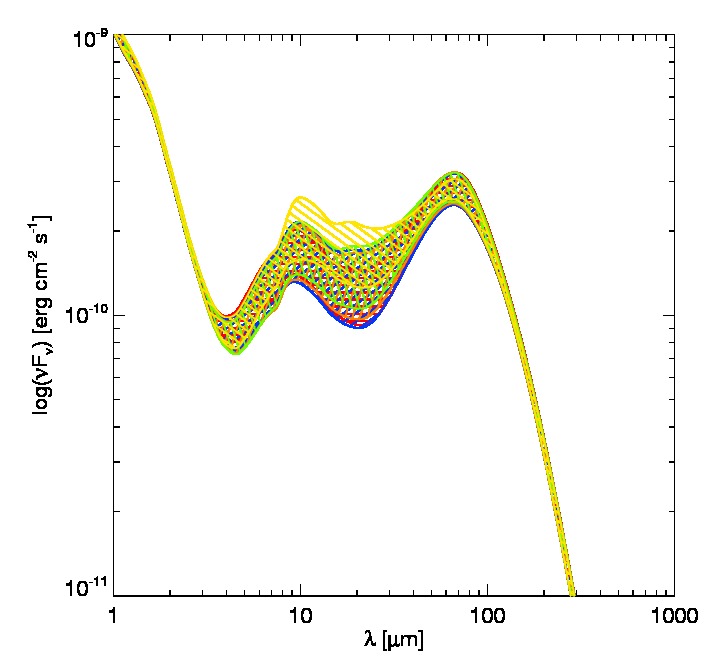
Figure 2: Average spectral energy distributions of models with $L_{\rm X}=0$ (red), $10^{29}$ (blue), $10^{30}$ (orange), $10^{31}$ (green), and $10^{32}$ erg s^-1 (yellow).

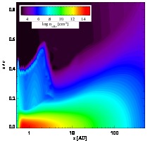
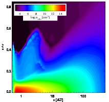
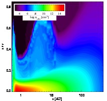
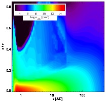
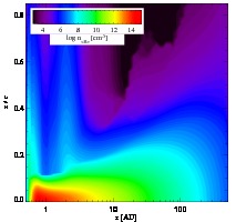
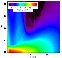
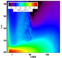
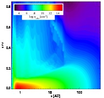
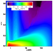
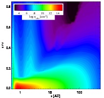
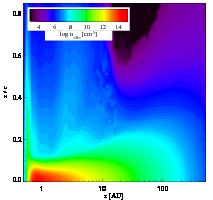
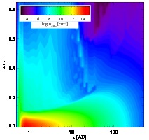
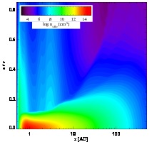
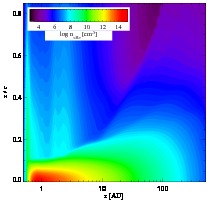
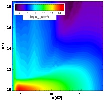
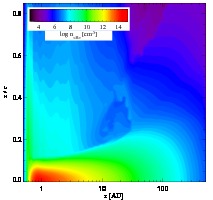
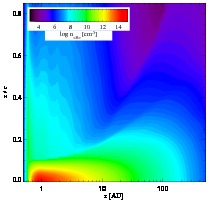
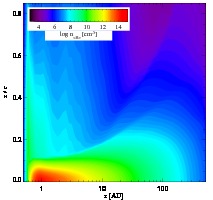
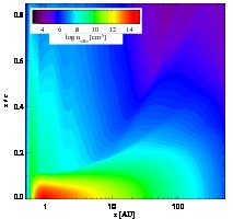
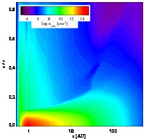
Figure 3: Total density: FUV luminosity increasing from $L_{\rm FUV}=10^{29}$ (left) to $10^{32}$ erg/s (right). X-ray luminosity increasing from $L_{x}=0$ (top) to $10^{32}$ erg/s (bottom).

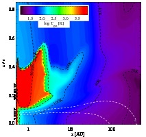
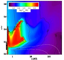
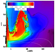
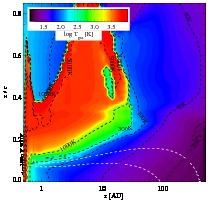
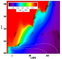
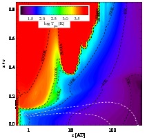
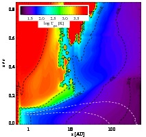
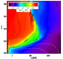
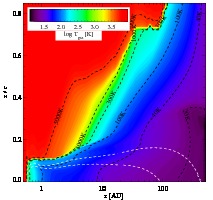
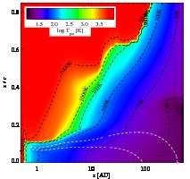
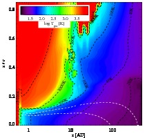
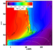
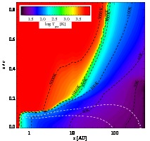
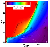
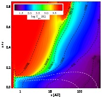
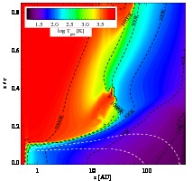
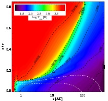
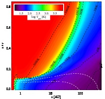
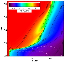
Figure 4: Gas temperature distribution: FUV luminosity increasing from $L_{\rm FUV}=10^{29}$ (left) to $10^{32}$ erg/s (right). X-ray luminosity increasing from $L_{x}=0$ (top) to $10^{32}$ erg/s (bottom). White contours represent the $A_{\rm v}=1$ and 10. The black contours represent the gas temperatures.

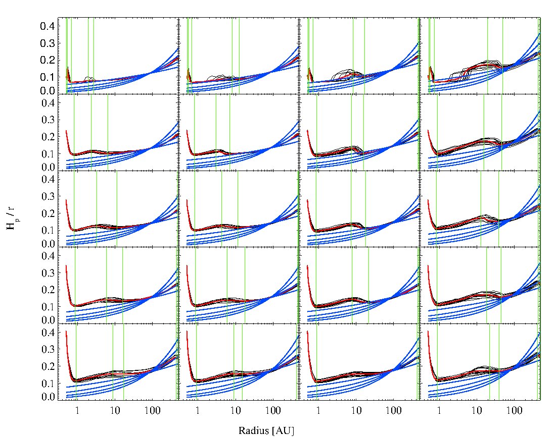
Figure 5: Scale height of the disk at $z/r=0.5$. The black lines show the 12 different models ($a_{\rm min}$, $a_{\rm max}$, and $\epsilon$), at a particular $L_{FUV}$ and $L_{\rm X}$. The vertical green lines indicate a maximum or minimum in the scale height. The red line is the average of the 12 models.

3 Disk thermal and density structure

The coupling of gas and dust to the radiation field determines the heating and cooling rates, which in return determine the pressure balance and structure of a disk. FUV and X-rays couple differently to the gas: FUV is absorbed by dust grains and ejects an electron with a small surplus of energy in the form of kinetic energy, which then consequently heats the gas. X-rays, on the other hand, are absorbed by the K-, L-, or M-shell of atoms, where no distinction is made as to whether this atom is part of a molecule, dust grain, or PAH. This assumption might overestimate the X-ray absorption cross section by a factor of approximately $\sim 2$ at energies $E<1$ keV, since we do not include self-shielding effects by large grains (see, e.g., Fig. 1 of Fireman, 1974). On the other hand, not much is known about gas and dust phase elemental abundances in disks. The observed abundance of, e.g., neon (dominating the X-ray absorption cross section between $\sim 0.9$ to $1.2$ keV, and, as such, the total absorption of our 1 keV thermal source), already varies over a larger range (see Glassgold et al., 2004, for a discussion on this topic). The electron that is ejected has a large energy capable of exciting, ionizing and heating the gas. The efficiency for X-ray heating is much larger, about 10 to 40 percent, depending on the ionization fraction of the gas, while that for FUV heating does not exceed one to three percent. The coupling of X-rays to gas is weaker than for FUV, due to the smaller cross section for the absorption, but the larger efficiency makes sure that it is an important heating source, even when the FUV excess is large. Their relative contribution to the energy budget will result in a different structure and emitted line fluxes. X-rays do not much affect the continuum fluxes, certainly less than $a_{\rm min}$, $a_{\rm pow}$, and $\epsilon$ (see Fig. 2). It shows that the fluxes change at most by a factor of three between $\lambda=5-100$ $\mu$m due to X-rays. The models with $L_{\rm X}=10^{32}$ erg s^-1 are affected most, and these high X-ray fluxes are rarely observed for T Tauri stars.

Woitke et al. (2009) have already pointed out that the cooling and heating balance is very important in determining the physical structure of the disk. They present in their Fig. 9 the density structures for (1) a model where the gas temperature is decoupled from the dust and (2) where the gas and dust temperature are coupled. Model 1 shows a very complex structure, where the gas is puffed up at the inner rim and a second bump in the density is seen at a radius $r\sim 10$ AU. Aresu et al. (2011) extended this model by including X-rays and showed for the particular model of Woitke et al. (2009) that the vertical extension inward of 10 AU becomes smoothed out for increasing X-ray fluxes and merges with the inner rim for the largest X-ray fluxes. A minimum in the vertical extension remains visible, though.

In Figs. 3 and 4, the density and temperature of the disk are shown for FUV luminosities ranging from $L_{\rm FUV}=10^{29}$, $10^{30}$, $10^{31}$, and $10^{32}$ erg/s (left to right) and for X-ray luminosities $L_{\rm X}=0$, $10^{29}$, $10^{30}$, $10^{31}$, and $10^{32}$ erg/s. There are 12 different possible variations with these X-ray and FUV luminosities (due to the variations in $a_{\rm min}$, $a_{\rm max}$, and $\epsilon$); as a baseline model, we always show the models with $a_{\rm min}=0.1$ $\mu$m, $\epsilon=1.5$, and $a_{\rm pow}=3.5$.

3.1 Density distribution

Because density and temperature structure are directly related and we assume hydrostatic equilibrium, many of the effects that are seen in the density structure will show up in the temperature structure as well. The FUV-only models show that the inner rim becomes higher and broader for increasing luminosity. The disk right behind the inner wall is shielded, and a second, vertically more extended density structure thus appears at radii between $r=2$ and 6 to 30 AU (depending on the FUV luminosity).

The X-rays have a different effect on the density structure. While the peak of the second bump in the density structure appears at larger radii for higher FUV luminosities, the X-rays mostly affect the region within 5 AU. The second bump behind the inner rim expands to smaller and smaller radii for increasing X-ray luminosities (while keeping FUV the same), and the absolute densities become higher (from $n\sim 10^{6}$ to $10^{8}$ cm^-3). Eventually, the puffed-up inner rim and the second bump merge. At the highest FUV luminosity, the merging of the two density structures occurs at the smallest X-ray luminosity.

3.2 Temperature structure

When only FUV is included in the models, we find that the temperature structure of the disk shows an inversion in the vertical direction: The temperature reaches a maximum at a certain relative height $z/r$ and shows a fast drop above it. For example, the models with $L_{\rm FUV}=10^{29}$ erg/s show a region with temperatures $T>1000$ K out to a radius $r\sim 3$ AU and between relative heights $z/r\sim 0.1$ to 0.4. Noticeable is also that the hot region extends to a slightly higher relative height at the inner rim (up to $z/r=0.45$) and at a radius $r=3$ AU (out to $z/r=0.55$). This is the result of shielding; the disk surface is less heated right behind the inner rim. For larger FUV luminosities, shielding effects are even more prominent and the drop in temperature right behind the inner rim is increasingly pronounced.

Adding X-ray heating changes this picture. These models show a much more extended region with temperatures higher than $T>1000$ K, even when the X-ray luminosity is much smaller than the FUV luminosity. At radii $r<5-10$ AU, the inversion layer disappears and the temperature just smoothly increases toward larger $z/r$. At larger radii ($r>10-20$ AU), the inversion layer only disappears when the X-ray luminosity is at least ten percent of the FUV luminosity. In models where the X-ray luminosity is much smaller, temperature distribution is also affected (or even dominated) by the FUV. An example is $L_{\rm FUV}=10^{32}$ erg/s in combination with $L_{\rm X}=10^{29}$ erg/s. Although the inversion layer disappears at small radii ($r<5$ AU), it is still present at larger radii.

3.3 Heating and cooling processes

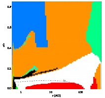
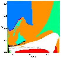
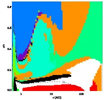
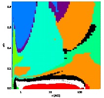
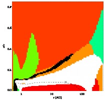
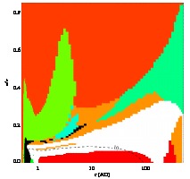
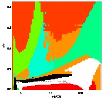
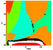
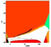
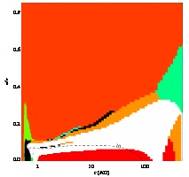
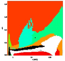
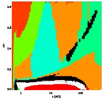
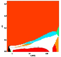
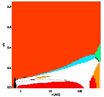
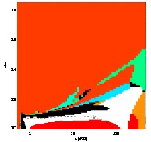
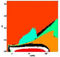
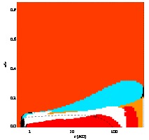
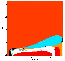
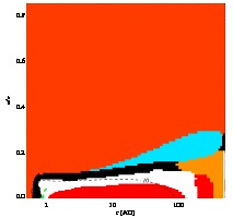
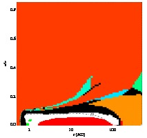
Figure 15: Main heating sources throughout the disk: FUV luminosity increasing from $L_{FUV}=10^{29}$ (left) to $10^{32}$ erg/s. X-ray luminosity increasing from $L_{x}=0$ to $10^{32}$ erg/s. background heating by [CII] (blue), PAH heating (orange), photo-electric heating (dark purple), X-ray Coulomb heating (light red), heating by collisional de-exciation of H₂ (blue-green), CI ionization heating (green-blue), infrared background by CO ro-vibrational lines (black), heating by thermal accomodation grains (white), cosmic ray heating (red), X-ray H₂ dissociation heating (light blue), free-free absorption (green), background heating by FeII (light green), background heating by SiII (green-yellow), infrared background heating by H₂O rotational transitions (yellow), heating by H₂ formation on dust (dark blue), and background heating by [OI] (purple).

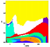
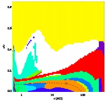
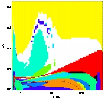
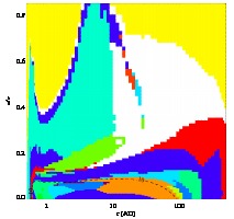
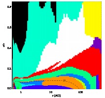
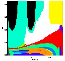
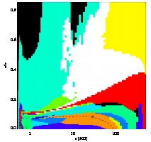
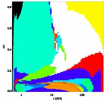
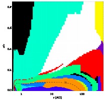
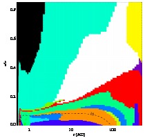
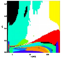
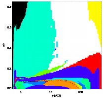
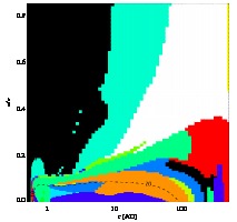
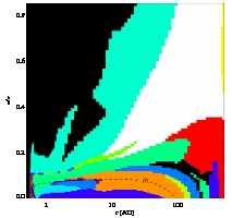
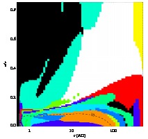
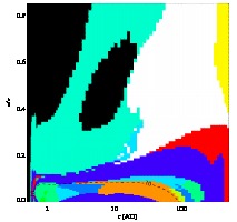
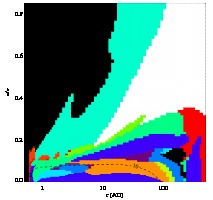
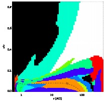
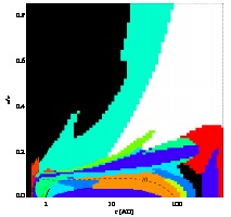
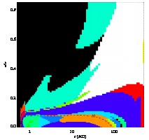
Figure 16: Main cooling sources throughout the disk: FUV luminosity increasing from $L_{FUV}=10^{29}$ (left) to $10^{32}$ erg/s. X-ray luminosity increasing from $L_{x}=0$ to $10^{32}$ erg/s. Lyman $\alpha$ cooling (black), [FeII] line cooling (blue-green), [OI] line cooling (white), [CII] line cooling (yellow), CO rotational and ro-vibrational cooling (red), H₂O rotational cooling (green-blue), OH rotational cooling (light green), HCN line cooling (dark purple), [CI] line cooling (light purple), HNC line cooling (blue), cooling by thermal accomodation on grains (dark blue), CS line cooling (yellow-green), H₂ line cooling (light blue), chemical cooling (red-orange), and free-free emission (green).

Temperature and density structure are in the end determined by the balance between the heating and cooling processes. Line cooling processes (except Lyman $\alpha$ and [OI] 6300Å line cooling) are treated in an escape probability approximation. Before solving the equations for statistical equilibrium, a global continuum radiation transfer calculation is done to estimate the background mean intensities for the radiative excitation and de-excitation rates. Other heating and cooling processes are approximated by an analytical expression. Over 50 different heating and 50 different cooling processes are included in the code. Except for the treatment of X-ray related heating processes, which are described in Aresu et al. (2011), we refer to Woitke et al. (2009, 2011) for a more detailed description. The reason that so many processes are included is that they each play a significant role, depending on the ambient density and radiation field (FUV, X-rays, cosmic rays), which vary over many orders of magnitude. It is beyond the scope of this paper to describe all these processes in detail for the models. However, we do present the dominant heating and cooling processes in Figs. 15 and 16 for the models for which we are showing the temperature and density structure.

First, we consider the FUV-only models. At the lowest FUV luminosity $L_{FUV}=10^{29}$ erg s^-1, there are three main heating process in the unattenuated part of the disk, namely, background heating by C⁺ at the lowest densities, $n_{H}=10^{5}$ cm^-3 (dark blue), PAH heating within the inner rim and the second extension of the disk (orange), and heating by carbon ionization in the outer disk (blue-green). Increasing the FUV field makes the picture more complicated. Heating by collisional de-excitation of H₂ becomes important in the second bump (light blue), while background heating by FeII is dominant at the inner rim. Locally, other processes, such as photo-electric heating, are important. Going to the more shielded regions of the disk, there is roughly a three-layered structure of dominating heating processes: (1) infrared background heating CO ro-vibrational transitions (black), (2) slightly deeper in the disk heating by thermal accomodation on grains (white), and (3) in the mid-plane cosmic ray heating (red). This three-layered structure becomes more confined toward the mid-plane for higher FUV luminosities.

X-ray Coulomb heating dominates in the upper part of the disk, when the FUV to X-ray luminosity $L_{\rm FUV}/L_{\rm X}\leq 1$. When it is higher than one, X-ray Coulomb heating is restricted to the higher regions of the disk. Adding X-rays increases the temperature significantly in the disk, making [FeII] also dominant in large parts of the second-density extension at the lowest X-ray luminosity, $L_{X}=10^{29}$ erg s^-1. For large X-ray luminosities, the structure of heating sources becomes less complicated. The entire unshielded part of the disk is dominated by X-ray Coulomb heating, followed by the three-layered structure described above (CO ro-vib, thermal accommodiation on grains, cosmic ray). For the highest two X-ray fluxes, an additional layer with X-ray H₂ dissociation heating as the main heating source is located on top of this three-layered structure.

In the FUV-only case, there are three main coolants in the unattenuated part of the disk: C⁺ line cooling (yellow), [FeII] line cooling (blue-green), and [OI] line cooling. The size of the region, where [FeII] line cooling dominates expands for higher FUV luminosities, while reducing the size of region where [OI] line cooling dominates. When X-rays are added, the region where C⁺ line cooling dominates is pushed to the outer part of the disk. Temperatures are much higher in the upper part of the disk, and as a result Lyman $\alpha$ cooling (black) dominates in increasingly larger regions of disk, when X-ray luminosities become larger. At the highest X-ray luminosities, we find a three-layered structure of Lyman $\alpha$ cooling, [FeII] line cooling, and [OI] line cooling. The shielded region of the disk shows a layered structure. CO ro-vibrational (red) and H₂O rotational cooling (green-blue) are on top. Closer to mid-plane, several smaller regions have their own major coolant, such as HCN (purple), and HNC (orange).

3.4 Vertical scale height

Another way to show the combined effects of X-rays and FUV on the disk structure is by comparing the scale vertical height. Our definition is the same as the one used by Woitke et al. (2009), and is approximately (i.e., assuming $z\ll r$) given by

$$\left(\frac{H}{r}\right)^{2}\simeq\frac{2rc_{T}}{GM_{\star}},$$ (1)

where $H$ is defined as $\rho(z)\approx\rho(0)\exp(−z^{2}/H^{2})$ and $c_{T}$ is the isothermal sound speed. As mostly the disk atmosphere is affected by the FUV and X-ray irradiation, we plot $H/r$ at the relative height $z/r=0.5$ in Fig. 5. In each panel, we overplot the scale height for all the different parameters in black (twelve models in total), and the red line is the average. Four blue lines are overplotted, indicating flaring index $H/r\propto r^{p}$ with $p=0.15-0.45$, where the lines are normalized to the vertical scale height at $r=100$ AU.

A number of things stand out in these plots: (i) The vertical scale height of the inner rim is mostly affected by the X-rays, and almost no response is seen for different FUV luminosities. The scale height is $H/r=0.15$ without X-rays at the inner rim, and it increases to $\sim 0.4$ at $L_{X}=10^{32}$ erg/s. (ii) The second bump also shows up when plotting $H/r$ and slowly moves outward for increasing X-ray luminosities. (iii) The flaring index $p$ is 0.25 in the outer disk ($r>100$ AU), similar to the $2/7$ exponent found by Chiang & Goldreich (1997). The vertical scale height in the inner disk is elevated, compared to the outer disk. (iv) The $H_{0}/r\approx 0.1$ and $0.18$ at $r_{0}=100$ AU and $z/r=0.1$ and 0.5, respectively. For a direct comparison to Chiang & Goldreich (1997), we measure $H_{0}/r$ at $r_{0}=10$ AU, because the approximation of the disk dust temperature being vertically isothermal does not hold in our models at the larger distances. We find a value $H_{0}/r\approx 0.04$, which is very similar to Chiang & Goldreich (1997), after correcting for the stellar mass and their definition of the scale height. (v) The merging of the inner rim with the second bump is clearly visible, as changes in the vertical scale height in the inner disk ($r=1-10$ AU) become more gradual for larger X-ray luminosities.

4 The chemical balance in the disk

The combined effects of X-rays and FUV irradiation on the disk are discussed in this section. The density structure is in pressure equilibrium as discussed in the previous section and is altered due to irradiation effects. The chemical rates are density dependent, and as such the pressure balance also influences the abundances of the species.

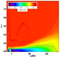
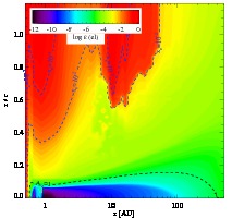
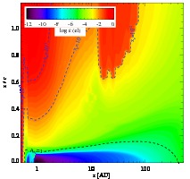
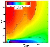
Figure 6: Electron abundance: FUV luminosity is fixed at $10^{31}$ erg/s. X-ray luminosity increases from $L_{x}=0$ (left) to $10^{32}$ erg/s (right). The black dashed line indicates $A_{\rm V}=1$. The blue lines mark the ionization fractions $x_{e}=10^{-2}$ and 10^-1.

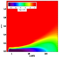
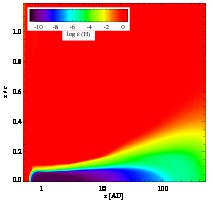
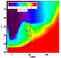
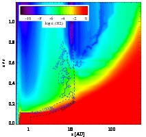
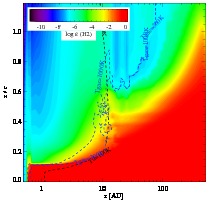
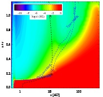
Figure 7: Abundance structure of atomic (top) and molecular (bottom) hydrogen. FUV and X-ray fluxes are the same as in Fig. 6. The blue contours indicate the gas temperature $T_{\rm gas}=300$ and 1000 K. The black line indicates $T_{\rm dust}=100$ K.

4.1 Electron abundances

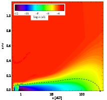
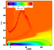
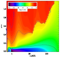
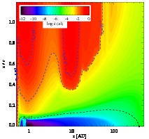
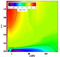
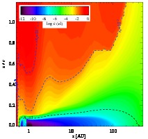
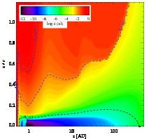
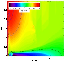
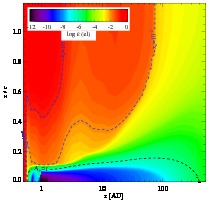
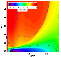
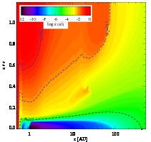
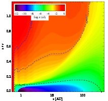
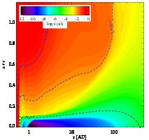
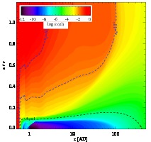
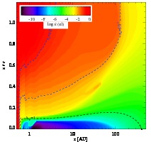
Figure 17: Electron abundance: FUV luminosity increasing from $L_{FUV}=10^{29}$ (left) to $10^{32}$ erg/s (right). X-ray luminosity increasing from $L_{x}=0$ (top) to $10^{32}$ erg/s (bottom).

The main electron donor in a FUV-only chemistry is atomic carbon, because the incident FUV radiation field is not capable of ionizing atomic hydrogen, leaving cosmic rays as the only ionization source of atomic hydrogen. As a result, the maximum electron abundance will not be higher than $x_{\rm e}\sim 10^{-4}-10^{-3}$, as can be seen in Figs. 6 and Fig. 17. The maximum electron abundances occur where the disk is unshielded to the radiation source. The inner rim has significant ionization fractions ($x_{\rm e}\sim 10^{-4}-10^{-3}$) all the way down to the midplane of the disk, while further out the electron abundances are only this high at densities $n<10^{7}$ cm^-3. The drop of the electron abundances below $x_{\rm e}<10^{-6}-10^{-5}$ for higher densities nicely coincides with the $A_{V}=1$. Closer to the midplane, when the radiation becomes more shielded and densities are higher, the electron abundance exhibits a fast drop. This is the result of a combination of a decreasing ionization rate, $\zeta\propto n$, and an increasing recombination rate, $k_{\rm rec}\propto n^{2}$. The abundance drop becomes more gradual at larger radii, which is a result of lower ambient densities and thus lower recombination rates. The region where the transition occurs is moving slightly toward smaller relative heights, when FUV fluxes are higher. The change in the transition location is not much due to the sharp increase of the density toward the midplane ($k_{rec}\propto n^{2}$): A relatively small increase in the density already compensates for larger FUV fluxes.

This picture changes quite significantly when the radiation fields also contain X-rays. The absorption of an X-ray photon by an arbitrary species creates a fast electron that can produce many ionizations, e.g., a 1 keV electron is able to produce $\sim 27$ hydrogen ionizations. As a result, the electron abundances are much higher when X-rays are included. In the unattenuated part of the disk, ionization fractions are of the order $x_{e}\sim 10^{-2}-10^{-1}$ (contours for $x_{e}=10^{-2}$ and $10^{-1}$ are indicated). They can even be higher than $x_{\rm e}>10^{-1}$ at very small radii ($r<0.5$ AU) and high relative heights ($z/r\gtrsim 0.5$). Here, low densities ($n_{\rm H}<10^{7}$ cm^-3) and high temperatures ($T\gg 5000$ K) reduce the recombination rates. Recombination rates decrease with temperature up to $T\sim 10000$ K because they are dominated by radiative recombination, which scales as $k_{\rm rec}\propto n_{e}n_{i}(T/10^{4})^{-X_{\rm rad}}$, with $X_{\rm rad}\sim 0.6-0.9$. We find slightly higher ionization fractions than, e.g., Glassgold et al. (2004). Their calculation at $r=1$ AU (see their Fig. 4) is truncated at vertical column density $N_{\rm H}\approx 2\times 10^{18}$ cm^-2 and density $n_{\rm H}\approx 10^{7}$ cm^-3 . Ercolano et al. (2008) (their Figs. 1 and 2) show calculations for lower column densities and densities, and they find ionization fractions slightly higher than $x_{e}>1$ at 0.07 AU at vertical column densities $N_{\rm H}<10^{16}$ cm^-2. Both calculations are consistent with those presented here. The electron abundance structure looks a little counterintuitive, especially for the lowest two X-ray fluxes $L_{\rm X}=10^{29}$ and $10^{30}$ erg/s. The region with very high ($x_{\rm e}\approx 10^{-2}-10^{-1}$) becomes smaller for increasing FUV luminosities (Fig. 17). This is because the inner rim is puffed up more and even merged with the second bump for the highest FUV fluxes. The densities are elevated to $n_{\rm H}=10^{8}$ cm^-3 in these regions, and the recombination rates are orders of magnitude higher as a result. The outer disk is shielded from radiation. The regions with very high ionization fractions ($x_{\rm e}>10^{-2}$) are of similar size for all FUV luminosities only for the highest X-ray luminosity (see Fig. 17).

When the ionization fraction is increased by orders of magnitude, the gas shows a radically different chemistry, as it will be dominated by ion-molecule reactions. This will be discussed for some of the key species, and water in particular.

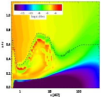
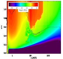
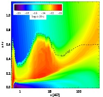
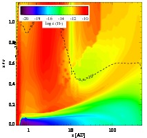
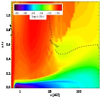
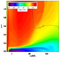
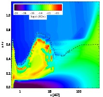
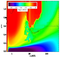
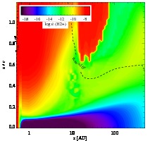
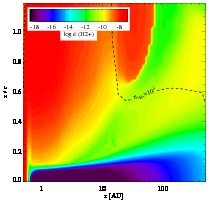
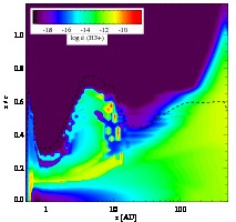
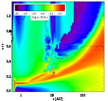
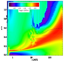
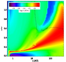
Figure 8: Abundance structure of H⁺, H^-, H${}_{2}^{+}$, and H${}_{3}^{+}$. FUV and X-ray fluxes are the same as in Fig. 6. Black contour indicates $n_{\rm H}=10^{5}$ cm^-3.

4.2 H and H₂ abundances

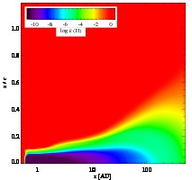
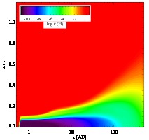
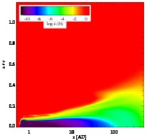
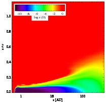
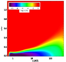
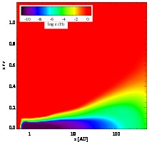
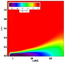
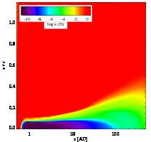
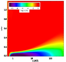
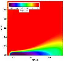
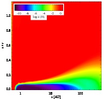
Figure 18: H abundances. FUV and X-ray fluxes are the same as Fig. 17.

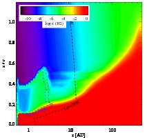
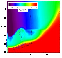
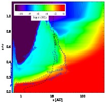
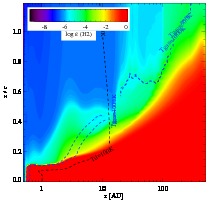
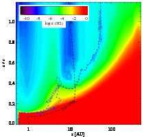
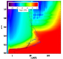
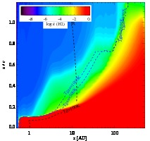
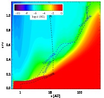
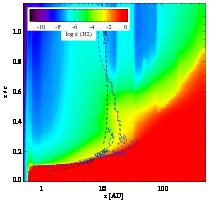
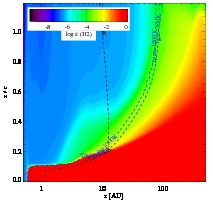
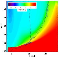
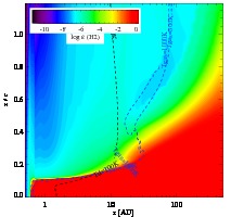
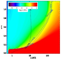
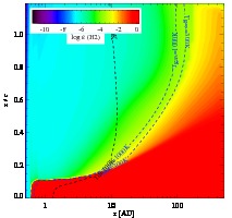
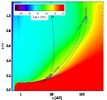
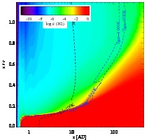
Figure 19: H₂ abundances. FUV and X-ray fluxes are the same as Fig. 17.

The abundance structure of atomic hydrogen is shown in the top panel of Fig. 7 (and also in Figs. 18 and 19). The highest abundances ($x_{\rm H}\gtrsim 10^{-2}$) are obtained in the unshielded region of the disk, where FUV and X-rays have high fluxes. At radii $r<0.6$ AU, the disk is atomic all the way down to the mid-plane of the disk, as it is directly exposed to the central source. At larger radii, the atomic fraction drops below $x_{\rm H}\sim 10^{-2}$ and makes a transition to molecular hydrogen at a relative height of $z/r\sim 0.1$ between $r\sim 0.6-5$ AU. The transition occurs at increasingly larger relative heights at larger distances to the central source, and it is at approximately $z/r\sim 0.4-0.5$ (depending on the X-ray flux) at a distance $r\sim 100$ AU. The transition occurs at slightly smaller relative heights at larger X-ray fluxes.

The formation of H₂ on grains is extremely efficient ($\sim 1$) when the dust temperatures are not high ($T_{\rm dust}\sim 10-50$ K (Cazaux & Tielens, 2004). At dust temperatures higher than $T_{\rm dust}>100$ K, the H₂ efficiency drops rapidly and H₂ formation on dust does not occur at $T_{\rm dust}>1000$ K. H₂ is also formed through the H^- route, $\rm H^{-}+H\rightarrow H_{2}+e^{-}$, especially when X-rays are present, and the fractional abundance of electrons is relatively high (and thus also H^-). It is possible to maintain an efficient route to form molecular hydrogen in the gas phase at high temperatures, $T_{\rm gas}>300$ K and $T_{\rm dust}>100$ K (see contours in Fig. 7). Also FUV is much more efficient in destroying H₂, than X-rays. The FUV photo-dissociates H₂ ($\rm H_{2}+$ FUV photon $\rightarrow\rm H_{2}^{*}\rightarrow H+H$). X-rays predominantly ionize molecular hydrogen indirectly by collisions with fast electrons produced after an X-ray absorption ($\rm H_{2}+e^{-*}\rightarrow H_{2}^{+}+e^{-}+e^{-*}$), while only a small fraction of H₂ is dissociated in this process. After ionization, H₂ is able to reform H₂ through $\rm H_{2}^{+}+H\rightarrow H_{2}+H^{+}$, but it will also be able to form H${}_{3}^{+}$ through the reaction $\rm H_{2}^{+}+H_{2}\rightarrow H_{3}^{+}+H$. This particular species is key in forming molecules through ion-molecule reactions. Because X-rays are destroying H₂ less efficiently and can provide an environment to form H₂ in the gas-phase, a fast ion-neutral chemistry results, which makes it possible to form molecules (and maintain significant abundances) at much higher temperatures than when only FUV is present.

The bottom panel of Fig. 7 presents the abundances of H₂. It shows that the H₂ abundance in the warm atmosphere of the disk is largest for the highest X-ray fluxes (as high as $x_{\rm H_{2}}\sim 10^{-6}$ in the region directly exposed to the central source at $r=0.6$ AU). This is the result not only of the processes described above, but also of the scale height of the inner rim, which increases with X-ray luminosities, an effect described in the previous section.

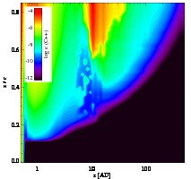
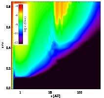
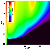
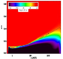
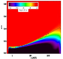
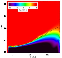
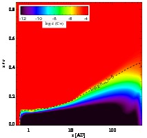
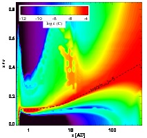
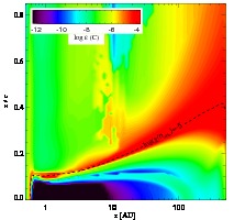
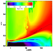
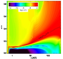
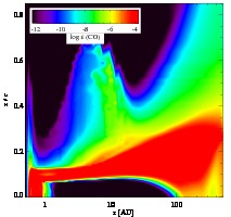
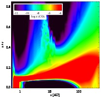
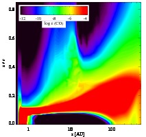
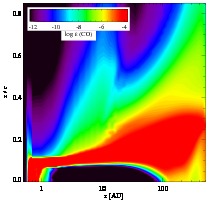
Figure 9: C²⁺, C⁺, C, CO abundances. The black dashed line indicates $\log(\chi/n_{\rm H})=-5$. Fluxes are the same as Fig. 6.

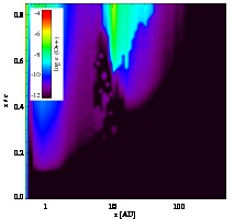
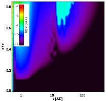
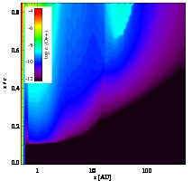
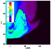
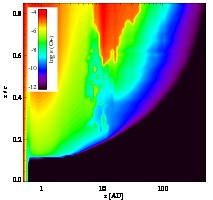
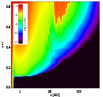
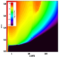
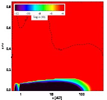
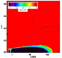
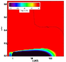
Figure 10: O²⁺, O⁺, and O abundances. Fluxes are the same as in Fig. 6. The black contour in the lower panel indicates the critical density of the [OI] 63 $\mu$m line.

4.3 H⁺, H^-, H${}_{2}^{+}$, and H${}_{3}^{+}$ abundances

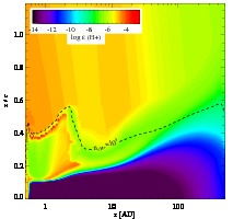
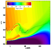
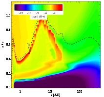
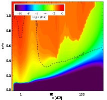
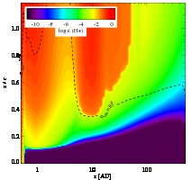
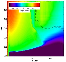
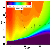
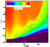
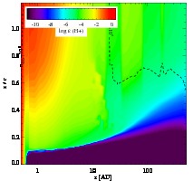
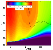
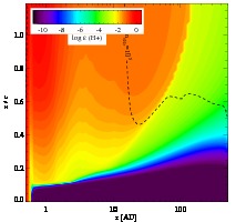
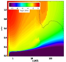
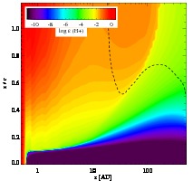
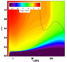
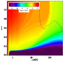
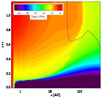
Figure 20: H⁺ abundances. FUV and X-ray fluxes are the same as Fig. 17.

The main drivers of the chemistry in the atmospheres of disks exposed to irradiation are ionic species, starting with H⁺, H${}_{2}^{+}$, and H${}_{3}^{+}$ (see also the discussion of the water chemistry). The H^- abundance structure is shown for completeness, since it can be important in the production of H₂ (see Fig. 8 and Figs. 20 to 23).

The abundance structure of ionized hydrogen shows abundances as high as $x_{\rm H^{+}}\sim 10^{-3}-10^{-2}$, even if there is only FUV irradiation. FUV is not able to photo-ionize atomic hydrogen, and hydrogen ionization is solely done by cosmic rays. This only happens at very low densities ($n<10^{4}$ cm^-3), though. Once densities of the order of $n\sim 10^{5}$ cm^-3 are reached, the ionized hydrogen fractions are closer to $x_{\rm e}\sim 10^{-5}-10^{-4}$ or smaller. The ionization balance is regulated by the charge exchange reaction $\rm H+O^{+}\leftrightarrow H^{+}+O$. The backward reaction has an energy barrier of $T=227$ K, so the ratio of O⁺ with respect to H⁺ decreases with temperature. The charge exchange rates are much faster than the photo-ionization reaction or the recombination rates of the species. The amount of H⁺ is thus directly coupled to the production rate of O⁺, which is also produced by cosmic ray ionization. Even when X-ray ionization determines the ionization balance of the gas, the charge exchange rates are much faster than the primary and secondary X-ray ionization rates of the species, and the ion abundances are directly coupled. X-rays produce much higher fractions of H⁺ (as high as $x_{\rm H+}>0.1$ at the lowest densities). The abundance structure strongly resembles that of the electrons, although the H⁺ abundance drops faster closer to the mid-plane, and other species such as Na⁺ take over as electron donor (see also Ádámkovics et al., 2011).

Once the gas gets more shielded to the radiation, it has higher abundances of molecular species (see, e.g., Fig. 19). In those regions, H⁺ can also be produced by other reaction paths, such as $\rm CO^{+}+H\rightarrow CO+H^{+}$ when only FUV is present and secondary X-ray ionization of H₂ when X-rays are present as well. Once cosmic ray ionization is the dominant source of ionization, H⁺ is produced by cosmic ray ionization of H₂ or charge exchange with He⁺.

The H^- ion is produced by cosmic ray ionization ($\rm H_{2}+CR\rightarrow H^{+}+H^{-}$) or by radiative recombination (${\rm H}+{\rm e^{-}}\rightarrow{\rm H}^{-}+h\nu$). This last reaction is fairly slow at low temperatures due to temperature barriers, but it becomes important in the warm part of the atmosphere of the disk. When only FUV is irradiating the disk, the H^- abundance is high ($x_{\rm H^{-}}\sim 10^{-11}-10^{-10}$) at the inner rim and in the second bump extending out of the disk, and to a lesser extent in the transition zone from atomic to molecular gas. There are two reasons that there is not as much H^- at high altitudes in the disk. The first one is that the electron densities are two to three orders of magnitude lower. The second one is that the ambient temperatures are between 50 and 100 K, which is not very favorable as the reaction rate contains an energy barrier. At the inner rim and in the second bump, both temperatures ($T>1000$ K) and densities ($n>10^{7}$ cm^-3, and thus also electron densities) are much higher. When X-ray irradiation plays a role, the abundances structure changes a lot. The temperatures are in excess of $T>1000$ K to large relative heights (see Fig. 4), and electron abundances are much higher (due to higher ionization rates and slower recombination rates). Especially when X-ray luminosities exceed $L_{X}>10^{30}$ erg/s, the relative abundances of H^- are one to three orders of magnitude higher (close to $x_{\rm H^{-}}\sim 10^{-8}$). In the FUV case, the H^- route to form H₂ is at least three orders of magnitude lower than the formation route on dust grains. It becomes a significant contributor ($\sim 30\%$) to the total H₂ formation rate at the highest X-ray luminosities when these extreme ($x_{\rm H^{-}}\sim 10^{-8}$) abundances are reached, and at the same time, H₂ formation on dust is quenched by high dust temperatures.

H${}_{2}^{+}$ is formed by cosmic ray ionization ($\rm H_{2}+CR\rightarrow H_{2}^{+}+e^{-}$) in the regions where the gas is molecular and shielded from FUV and X-ray radiation. When the H₂ abundance is high ($x_{\rm H_{2}}\sim 0.5$), however, the H${}_{2}^{+}$ is quickly transformed to H${}_{3}^{+}$ ($\rm H_{2}^{+}+H_{2}\rightarrow H_{3}^{+}+H$). It is above this layer, that the H${}_{2}^{+}$ abundance is increasing. Here, the gas is more exposed to radiation (FUV or X-rays). If X-rays are present, H₂ is ionized through secondary ionizations. In the FUV-only case, where we do not have this last reaction, other routes contribute to the production of H${}_{2}^{+}$. One example is $\rm S^{+}+H_{2}\rightarrow H_{2}^{+}+S$. In the unshielded regions of the disk, where H₂ abundances are low ($x_{\rm H_{2}}<10^{-6}$), the only efficient way to form H${}_{2}^{+}$ is through radiative association ${\rm H^{+}}+{\rm H}\rightarrow{\rm H_{2}^{+}}+h\nu$. However, this is only efficient at relatively high temperatures ($T>5000$ K) and significant abundance levels of H⁺. In Fig. 8, the cation H⁺ is shown to be more abundant by orders of magnitude when X-rays are present. It is obvious that the production of H${}_{2}^{+}$ is much more efficient as well, and hence abundances $x_{\rm H_{2}^{+}}\sim 10^{-8}-10^{-7}$ occur in the high warm atmosphere of the disk. In the FUV-only case, there is only a significant abundance ($x_{\rm H_{2}^{+}}>10^{-12}$) in the inner rim and the second bump.

The dominant way to form H${}_{3}^{+}$ is through the ion-molecule reaction $\rm H_{2}^{+}+H_{2}\rightarrow H_{3}^{+}+H$. As a result, the H/H₂ transition layer and the region below is very suitable to produce large abundances: H₂ is present in reasonable amounts ($x_{\rm H_{2}}>10^{-5}-10^{-3}$, see Fig. 7), and radiation is available to produce H${}_{2}^{+}$ (see previous paragraph, and Fig. 8). Once the H${}_{2}^{+}$ drops below an abundance $x_{\rm H_{2}^{+}}<10^{-12}$, the H${}_{3}^{+}$ abundance also drops to values below $x_{\rm H_{3}^{+}}<10^{-11}$. Consequently, there is a distinct layer where H${}_{3}^{+}$ is formed in the most optimal way. We also saw that the H${}_{2}^{+}$ is more efficiently formed when X-rays are abundantly present in the disk. The H${}_{3}^{+}$ abundances thus also significantly increase for larger X-ray luminosities and can be as high as $x_{\rm H_{3}^{+}}\gtrsim 10^{-8}$. In the FUV-only case, the size of the region where H${}_{3}^{+}$ is present in large abundances is smaller, and the maximum abundance is at least an order of magnitude lower compared to the models that include X-rays. It is a key species in driving ion-molecule chemistry, and so the chemistry with and without X-rays will obviously yield significantly different abundance structures.

4.4 C²⁺, C⁺, C and CO abundances

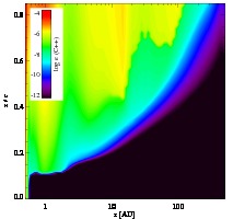
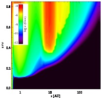
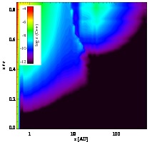
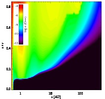
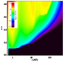
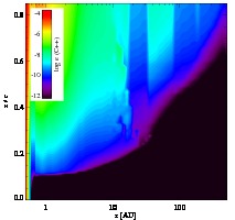
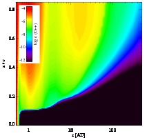
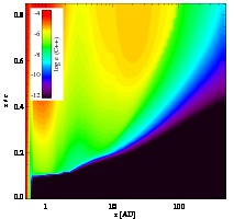
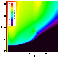
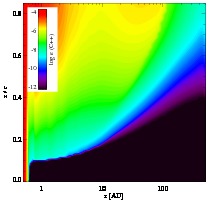
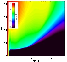
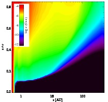
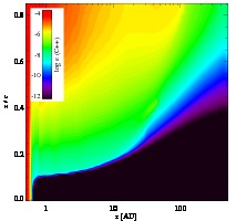
Figure 24: C²⁺ abundances. FUV and X-ray fluxes are the same as Fig. 17.

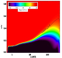
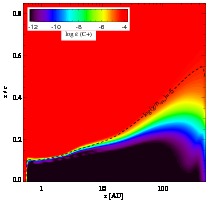
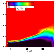
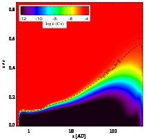
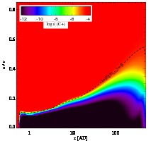
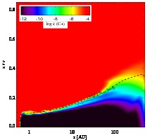
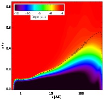
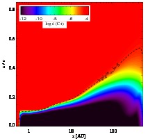
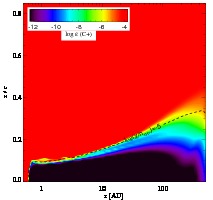
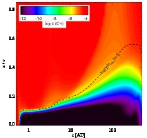
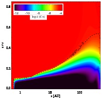
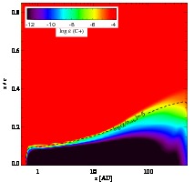
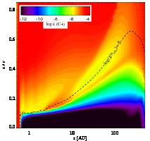
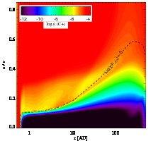
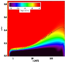
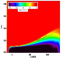
Figure 25: C⁺ abundances. FUV and X-ray fluxes are the same as Fig. 17.

The ionization potentials ($IP$) of the species C and C⁺ are $IP=11.26$ and 24.38 eV, respectively. While FUV photons can ionize neutral carbon, X-rays (or collisions with the resulting fast electrons) and/or cosmic rays are needed to reach a higher degree of ionization. As a result, the abundance patterns of the two species C⁺ and C²⁺ respond radically differently to the incident radiation field on the disk. The C²⁺ abundance pattern is, of course, strongly correlated with the X-ray luminosity, and C²⁺ is absent in models without X-rays. The region with significant C²⁺ abundances ($x_{\rm C^{2+}}>10^{-9}-10^{-8}$) extends to larger radii and smaller relative heights for higher X-ray luminosities, simply because there is more ionizing radiation available (and not inhibited by dust, since the dominant opacity is caused by the gas). However, the FUV plays an important role in shaping the disk and therefore indirectly affects the abundance distribution as well. The bump in the total H number density (see Fig. 3) extends to larger relative heights for larger FUV luminosities, thereby increasing the density at larger relative heights. This causes a larger attenuating column between the central source and the outer part of the disk, thus reducing the amount of ionizing photons. Furthermore, it allows H₂ to form at smaller radii. H₂ is very efficient in reducing C²⁺ by charge exchange reactions, such as $\rm C^{2+}+H_{2}\rightarrow C^{+}+H$. As a result, the FUV luminosity confines the C²⁺ to smaller radii (see Fig. 24). C⁺ is present throughout the unattenuated part of the disk. It has an abundance $x_{\rm C^{+}}\sim 10^{-4}$ down to the mid-plane in the inner rim ($r<0.6$ AU). Beyond this radius, carbon is only significantly ionized above a relative height $z/r\sim 0.1$ (at $r\sim 0.6$ AU), increasing to $z/r\sim 0.4$ at $r\sim 200$ AU. The width $\Delta z/r$, over which the transition from C⁺ to C and CO occurs, is larger toward the outer regions of the disk. Absolute densities of C⁺ and e^- in the inner disk are larger, and recombination rates scale with $n^{2}$. As a result, the transition from ionized to neutral carbon occurs abruptly, similar to the abundance drop of electrons (at approximately $z/r\sim 0.01$ at $r=1$ AU). However, in the outer disk ($r=200$ AU), the transition stretches out from $z/r\sim 0.04$ to 0.01. Although there are variations of a factor a few in the absolute abundance of C⁺, the overall appearance of the abundance structure is not significantly affected for different values of the X-ray and FUV luminosity (see Fig. 25).

The neutral carbon abundance pattern is very much affected by variations in the X-ray and FUV luminosities. In the case where only FUV is irradiating the disk, one finds a clear transition from C⁺ to C to CO (see Fig. 9), which is expected in a FUV-dominated PDR (cf. Hollenbach & Tielens, 1999). To guide the eye, we added a contour with value $\log(\chi/n_{\rm H})=-5$ (with $\chi$ the Draine field). This contour follows the C⁺/C/CO transition very well, indicating PDR physics. Neutral carbon is confined in a layer between the C⁺ and CO. This picture is more complicated when X-rays are added. Perhaps not entirely intuitive, the overall trend with increasing X-rays is that neutral carbon is more and more abundant in the unattenuated part of the atmosphere (as high as $x_{\rm C}\sim 10^{-5}-10^{-4}$). When X-rays are present, neutral carbon is higher by at least one to two orders of magnitude in abundance compared to models that exclude X-rays. The C and C⁺ ionization rates are of course higher, but the recombination rates are also higher owing to the increased electron abundances (although the higher temperatures reduce the recombination rates, as already pointed out in Sect. 4.1). This is because electrons are now also produced by, e.g., ionization of hydrogen and helium. The fact that C⁺ and C coexist in more or less equal amounts, when X-rays are dominating the ionization fraction of gas clouds, was already pointed out in papers by Maloney et al. (1996) (see their Figs. 3a and 4a) and Meijerink & Spaans (2005) (see their Figs. 3 and 4).

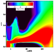
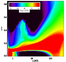
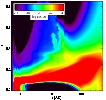
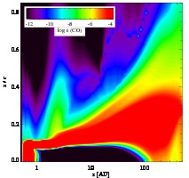
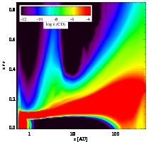
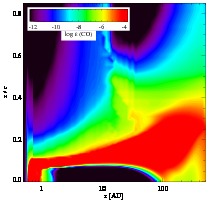
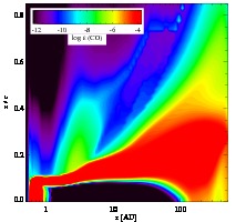
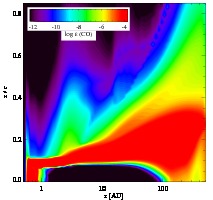
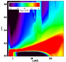
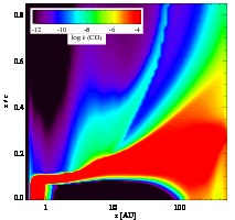
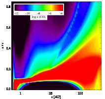
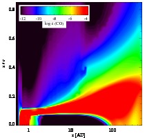
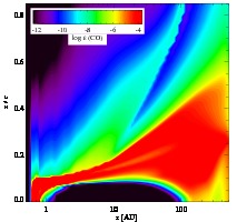
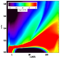
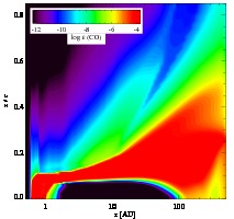
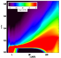
Figure 27: CO abundances. FUV and X-ray fluxes are the same as Fig. 17.

The bulk of the CO is situated in the shielded, optically thick part of the disk, and the total CO gas mass does not change when varying the FUV and X-ray radiation field. This molecule could thus serve as a tracer of the total mass of a protoplanetary disk, keeping in mind that the conversion factor depends on the amount of ice formation. A few details should be noted. There is a significant correlation between CO and OH in the unattenuated part of the disk (compare Fig. 27 with 31). A route to form CO is through the reaction $\rm C+OH\rightarrow CO+H$. While it is possible to obtain an abundance level of $x_{\rm CO}\sim 10^{-7}$ through this channel, it will never go up to $x_{\rm CO}\sim 10^{-4}$, because the OH abundance is $x_{\rm OH}\sim 10^{-7}$. As OH becomes less abundant for higher FUV luminosities (when X-rays are fixed), the CO also becomes less abundant and slightly more confined to the midplane. In addition, the the average abundance of CO drops slowly with increasing X-ray luminosity at the inner rim by destruction through ion-molecule reactions, such as $\rm CO+He^{+}\rightarrow C^{+}+O+He$. This could have an effect on the ro-vibrational lines that are predominantly produced in these regions.

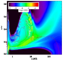
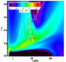
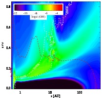
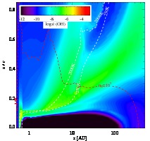
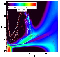
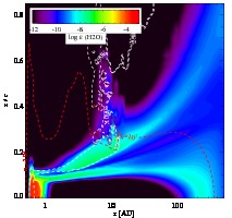
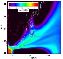
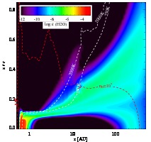
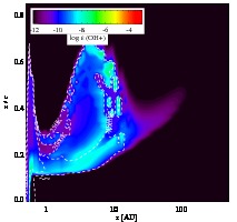
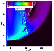
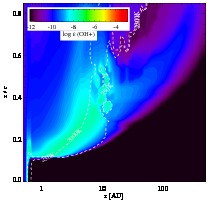
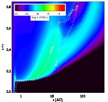
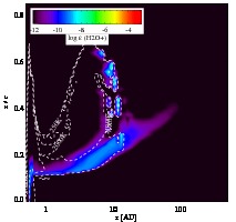
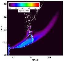
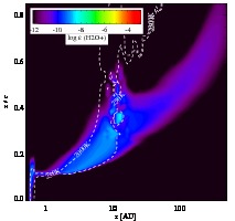
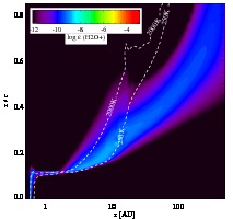
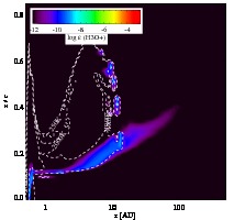
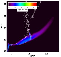
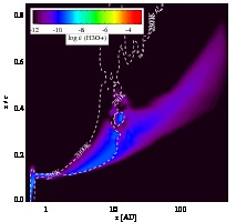
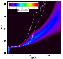
Figure 11: OH, H₂O, OH⁺, H₂O⁺, and H₃O⁺ abundances. Fluxes are the same as in Fig. 6. The white contours indicate gas temperatures of 250 and 2000 K. The red contour indicates the number density $n_{\rm H}=10^{6}$ cm^-3.

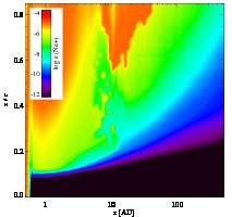
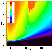
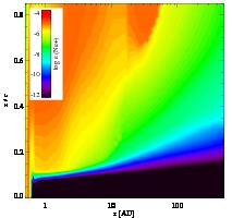
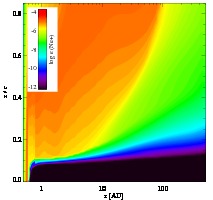
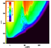
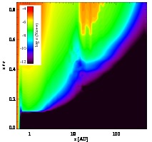
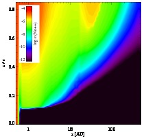
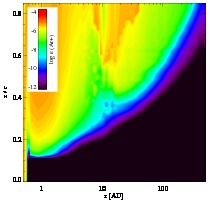
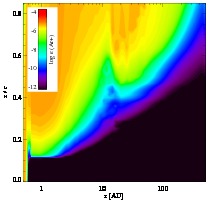
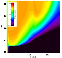
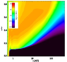
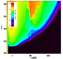
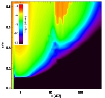
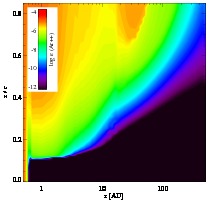
Figure 12: Abundance structure of selected heavy elements: Ne⁺ (top), Ne²⁺, Ar⁺, and Ar²⁺ (bottom). The FUV luminosity is fixed at $L_{\rm FUV}=10^{31}$ erg s^-1. X-ray luminosities vary between $L_{\rm X}=10^{29}$ and $10^{32}$ erg s^-1.

4.5 O²⁺, O⁺, and O abundances

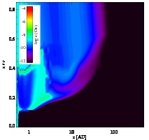
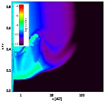
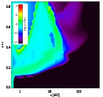
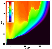
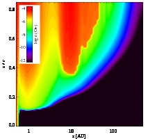
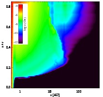
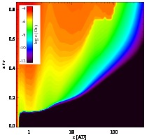
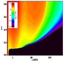
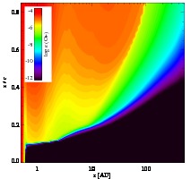
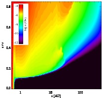
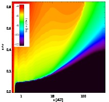
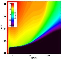
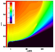
Figure 29: O⁺ abundances. FUV and X-ray fluxes are the same as Fig. 17.

The ionization potentials of O and O⁺ are $IP=13.68$ and 35.12 eV. Even the $IP$ of neutral oxygen is above the threshold of $IP=13.6$ eV, where neutral hydrogen blocks the radiation efficiently. The implications of this are seen in Fig. 10, where the abundances of neutral, singly and doubly ionized oxygen are shown for a FUV luminosity $L_{\rm FUV}=10^{31}$ erg s^-1 and all considered X-ray luminosities except $L_{\rm X}=10^{32}$ erg s^-1. The second row of Fig. 10 (and also Fig. 29 for variations with FUV luminosity) shows the abundance structure of singly ionized oxygen. Unlike the C⁺, the abundances of O⁺ do not exceed $x_{\rm O^{+}}\sim 10^{-8}-10^{-7}$ in the FUV-only case. The abundance of ionized oxygen is mostly set by the charge exchange balance with atomic hydrogen, while the ionization of both hydrogen and oxygen is entirely due to cosmic ray ionization. When X-rays are added, the abundances increase three to four orders of magnitude compared to the FUV-only case, even at low X-ray luminosities ($L_{\rm X}=10^{29}$ erg s^-1). Important to note is that the O⁺ is confined to smaller radii for larger FUV luminosities, which is also the case for C²⁺. This was discussed earlier in Sect. 4.4 and explained by the larger recombination rates due to higher densities in the upper atmosphere of the disk and the lower ionization rates due to shielding. The confinement to smaller radii is even stronger for the case of O²⁺, because this species is not affected by cosmic rays.

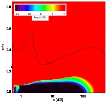
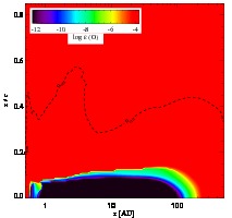
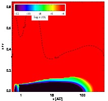
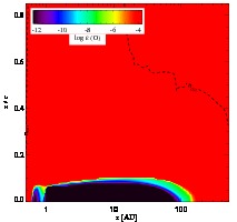
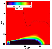
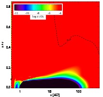
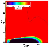
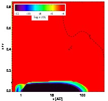
Figure 30: O abundances. FUV and X-ray fluxes are the same as Fig. 17.

The bottom panel of Fig. 10 shows the neutral oxygen abundance structure. The critical density is $n_{\rm crit}=5\times 10^{5}$ cm^-3 for the [OI] 63 $\mu$m line, which is indicated by a black dashed contour. This species does not change with X-ray luminosity. Neutral oxygen is the dominant oxygen carrier throughout the disk, except for those regions, where large fractions of the gas are frozen onto dust grains (i.e., the midplane). This species is very insensitive to changes in FUV and the ambient chemistry (see Fig. 30). The bulk of atomic oxygen is in LTE for the commonly observed [OI] 63 and 145 $\mu$m fine-structure lines and thus sensitive to the average temperature of the region that it is probing. As a result, the [OI] fine-structure lines have the potential to probe the total energy budget of the gas (the combined FUV and X-ray luminosity irradiating the disk). There will be an elaborate analysis of the oxygen fine-structure line emission in paper II.

4.6 OH, OH⁺, H₂O, H₂O⁺, and H₃O⁺ abundances

The water chemistry and its related species are significantly affected by X-ray irradiation. The physical circumstances in the disk change with radius $r$ and height $z$ due to radiation shielding and large differences in chemistry, which means that the X-ray and FUV energy deposition per particle, $H_{\rm X}/n$, and $\chi/n$ (with $\chi=1$ the interstellar radiation field as defined by Draine, 1978; Draine & Bertoldi, 1996, and integrated between 91.2 and 205 nm), and their relative ratio change over orders of magnitude in the disk. As a result, the main chemical pathways forming the molecules OH and H₂O change throughout the disk and the grid.

X-rays heat the gas and therefore the reaction rates with activation barriers increase. They also drive the ionization, which enhances formation routes through ion-molecule reactions. The formation of the neutral species OH and H₂O is either by the neutral-neutral reactions, $\rm H_{2}+O\rightarrow OH+H$, and $\rm H_{2}+OH\rightarrow H_{2}O+H$, or by recombination of ionized species, such as $\rm H_{3}O^{+}+e^{-}\rightarrow H_{2}O+H$ and $\rm H_{2}O^{+}+e^{-}\rightarrow OH+H$. Which of these pathways are dominating depends thus strongly on the temperature and ionization fraction. The routes through neutral-neutral reactions have activation barriers, making them efficient only when gas temperatures are sufficiently high, i.e., $T>200-300$ K. One way to increase the neutral-neutral route without the need of higher temperatures is by lowering the activation barrier, which can be done by exciting H₂ to a higher vibrational state after absorption of a FUV photon. At high relative heights ($z/r>0.5$), this reaction will dominate when only FUV photons are present. The ion-molecule chain is started with cosmic ray or X-ray ionization of H₂ and thus requires significant ionization rates.

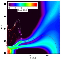
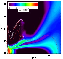
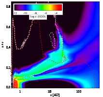
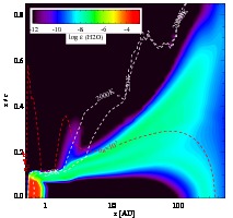
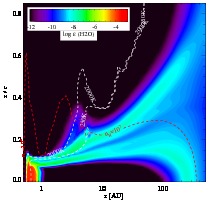
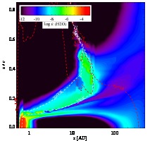
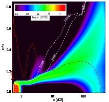
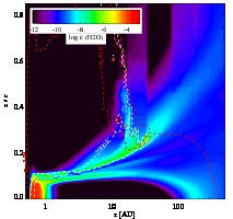
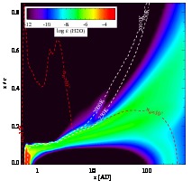
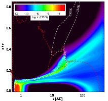
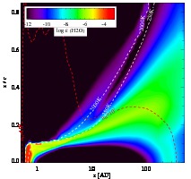
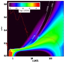
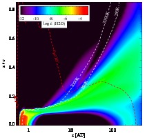
Figure 32: H₂O abundances. FUV and X-ray fluxes are the same as Fig. 17.

It turns out that the neutral-neutral reaction pathways dominate in the inner part of the disk ($r<5$ AU). The X-rays heat regions deeper in the disk, resulting in the production of a thick warm water layer. Although there is a larger fraction of X-rays ionizing the gas than when only FUV photons are present, the X-ray heating causes the neutral-neutral reactions to dominate. It is remarkable to note that in the outer region ($r\gtrsim 20$ AU) of the disk the ion-neutral reaction network dominates. This is because temperatures are too low for the neutral-neutral reaction pathways to occur. These combined effects become apparent in the distribution of the water throughout the disk, as shown in the second panel from the top in Fig. 11 (see also Fig. 32 for a more elaborate view on the effects of both FUV and X-rays). In the models without any X-rays (left-hand side), the water shows a strong abundance peak at the inner rim (all the way down to the midplane of the disk) and a warm water layer at a relative height $z/r\approx 0.1$, with an abundance of $x_{\rm H_{2}O}\sim 10^{-7}$, and a second water reservoir higher up in the disk. This reservoir is located at a relative height $z/r\sim 0.015$ at small radii ($r\sim 1$ AU), and at a relative height of $z/r\sim 0.5$ at a radius of $r\sim 100$ AU, thus following the flaring of the disk. These different water reservoirs were already noted by Woitke et al. (2009) for Herbig AeBe stars. An elaborate discussion on the formation of warm water reservoirs through (the dominant) neutral-neutral reactions and formation on dust grains in the inner regions of an X-ray irradiated disk is also outlined by Glassgold et al. (2009).

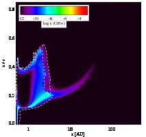
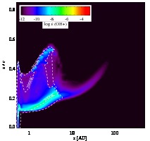
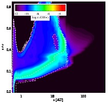
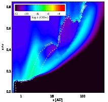
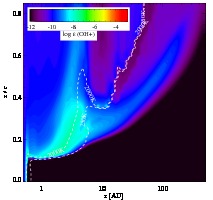
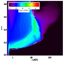
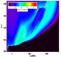
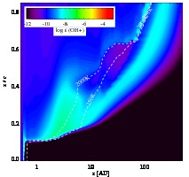
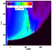
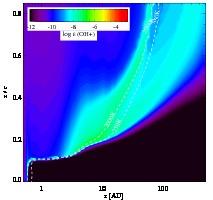
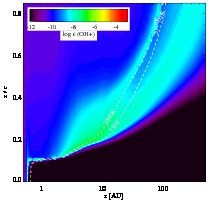
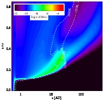
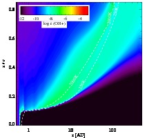
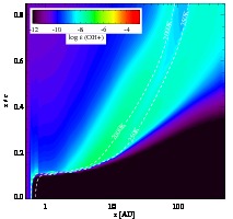
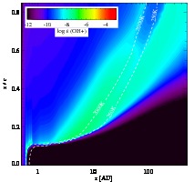
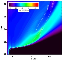
Figure 33: OH⁺ abundances. FUV and X-ray fluxes are the same as Fig. 17.

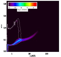
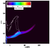
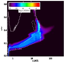
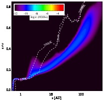
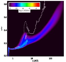
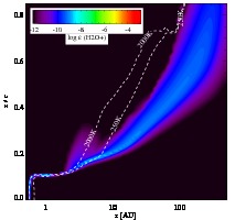
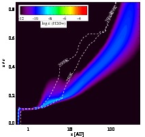
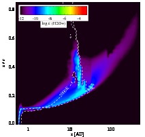
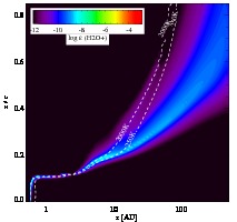
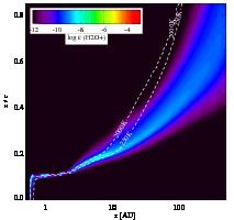
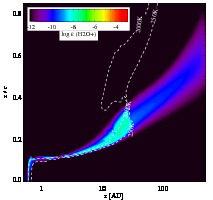
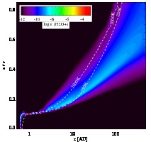
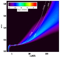
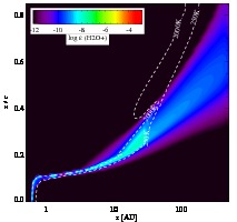
Figure 34: H₂O⁺ abundances. FUV and X-ray fluxes are the same as Fig. 17.

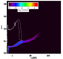
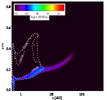
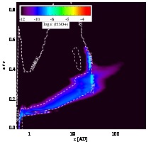
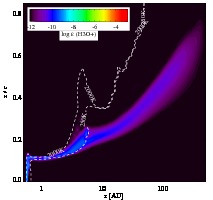
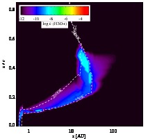
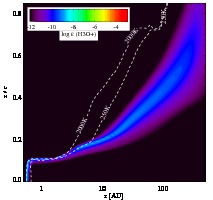
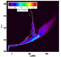
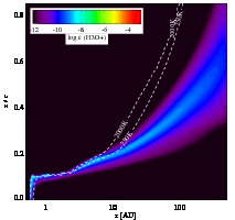
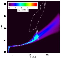
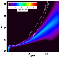
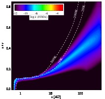
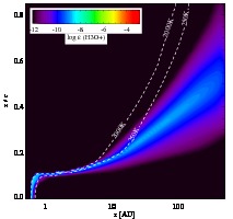
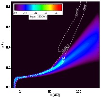
Figure 35: H₃O⁺ abundances. FUV and X-ray fluxes are the same as Fig. 17.

In the models where only FUV is included, the second layer is confined to the regions where temperatures are between $T\sim 300-1000$ K. The regions at higher temperatures are exposed to FUV fluxes that essentially destroy the water faster than it is formed. When X-rays are included, the second water reservoir extends to increasingly larger radii. Although there is water present in the FUV-only models out to radii $r\sim 200$ AU, the abundances are ultimately one to two orders of magnitude higher when X-rays are added. The additional water is increased since the ion-molecule chemistry is very effective in forming the water. This is illustrated in the third to fifth panel of Fig. 11 (and also Figs. 33, 34, and 35), where the changing abundance structures of the ionic species OH⁺, H₂O⁺, and H₃O⁺ are shown for various combinations of X-ray and FUV luminosities (appendix A only). The ionic species extend to larger radii for larger X-ray fluxes, but larger FUV fluxes decrease the extent. The fact that FUV confines the ionic species to smaller radii is an indirect effect, because FUV tends to puff up the upper layers of the disk and the density becomes higher at larger relative heights (see Fig. 3). These larger densities increase the recombination rates and reduce the abundances of these ionic species.

The first layer described above is located in those regions of the disk, where the conventional routes do not work anymore. Temperatures are too low and the ionization fraction is small. This is the region where more exotic reactions take over, such as $\rm NH_{2}+NO\rightarrow N_{2}+H_{2}O$. This layer has a smaller vertical extent in relative height for larger FUV fluxes. On the other hand, the second separate layer becomes thicker when X-rays are added. When the $L_{X}/L_{FUV}\gtrsim 1$ ratio, these two layers merge. The reason for the merging is the enhancement of the transient species OH⁺, H₂O⁺, and H₃O⁺ (see also Fig. 33, 34 and 35). As mentioned earlier, these species react sensitively to the presence of an ionization source and become increasingly abundant with higher X-ray fluxes.

The situation with OH is very similar. OH becomes more abundant in the outer disk, when X-rays are added. OH is located at higher altitudes in the disk (although there is also a large overlap with the regions where the water is located). For this reason, the effect of the X-rays on the abundance in the outer disk is not as pronounced as for water. The H₂ used in the neutral-neutral formation route of OH is on average at higher temperatures, so the relative contribution of the ion-molecule route is smaller.

4.7 Ar⁺, Ar²⁺, Ne⁺, and Ne²⁺ abundances

These species have ionization potentials that are larger than that for atomic hydrogen, with $IP=21.56$, 40.96, 15.76, and 27.63 eV for Ne, Ne⁺, Ar, and Ar⁺, respectively. The only way to produce these species is through direct (photon absorption and Auger effect) or indirect (fast electron collisions) ionization by X-rays. The presence of these ionized species is thus a direct result of the X-ray irradiation of the disk.

The models include a thermal source of temperature, $T_{\rm X}=1$ keV. As a result, the cross sections for neon are more favorable for direct ionizations than for argon. The cross section for the absorption is located at approximately $\sim 1$ keV for neon, while for argon it is $\sim 4$ keV. On the other hand, the rates for secondary ionizations are a little higher for argon, $\sigma(A)/\sigma({\rm H})=1.1$, 0.48, 3.7, and 1.8, with $A$ equal to Ne, Ne⁺, Ar, Ar⁺, respectively. Consequently, the total ionization rates are very comparable. However, there is one big difference in the chemical network of these species. The charge transfer rate of Ne⁺ with H₂ is very low ($k<10^{-14}$ cm³ s^-1), while the other ions have significant rates for charge exchange with molecular hydrogen. The Ne⁺ abundance structure thus extends to much smaller relative heights, down to $z/r\sim 0.01$, than Ar⁺, which is abundant above $z/r\sim 0.01-0.06$ at radii $r\gtrsim 10-200$ AU. The abundance structure of Ar⁺ is very similar to those for Ne²⁺ and Ar²⁺.

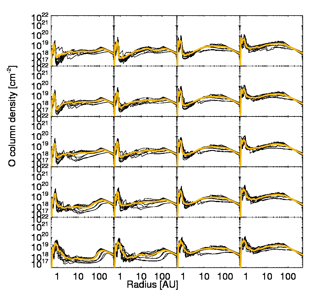
Figure 13: Radial column density distribution of O. FUV and X-ray fluxes are the same as Fig. 3.

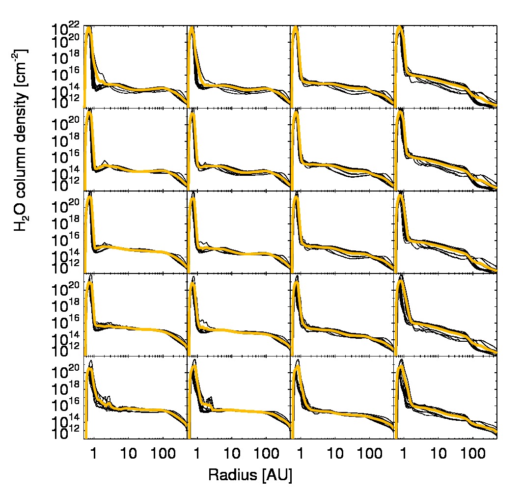
Figure 14: Radial column density distribution of H₂O. FUV and X-ray fluxes are the same as Fig. 3.

5 Radial column density profiles

Although the abundance distributions of species well illustrate the change in the chemistry due to different combinations of X-ray and FUV luminosities, it is necessary to look at the integrated properties of the disk that are observed by our telescopes. The focus in this is on the species C⁺, O, H₂O, and Ne⁺, as their line intensities and line profiles are extensively discussed the paper II. The figures show the average column density in yellow, while the black lines represent the 12 models at fixed FUV and X-ray luminosities. Changing parameters other than those for FUV and X-rays does not affect the results significantly.

C⁺ column density profile (Fig. 40): The column density of C⁺ is strongly related to the inicident FUV flux at the inner rim, where it increases from $N_{\rm C^{+}}\sim 10^{17}$ to $10^{19}$ cm^-2, when the FUV luminosity increases from $L_{\rm FUV}=10^{29}$ to $10^{32}$ erg s^-1. Right after the peak at the inner rim, there is a sharp drop in the column density, which is caused by the inner rim casting a shadow and therefore reducing ionizing radiation. A second peak in the column density profile is seen between $r\sim 5-10$ AU. The peaks moves to larger radii for higher FUV luminosities. The X-rays affect the column density profile in a different way. They reduce the minimum column density right after the inner rim and smooth the radial distribution. The combination of the highest FUV and X-ray fluxes gives the flattest distribution.

O column density profile (Fig. 13): The column density profiles of neutral oxygen do not change as much as those for C⁺. The maximum column density, $N_{\rm O}\sim 3-10\times 10^{19}$ cm^-2, is located right behind the inner rim and only varies with a factor of at most ten, which is again caused by the FUV irradiation. The width of the oxygen column density peak broadens a bit for higher FUV and X-ray fluxes. This makes the mininum in the column density less prominent in the radial column density profile. Because the column density is not very affected by radiation, it is a clean probe of the properties of a disk temperature ([OI] fine-structure lines), since there are no strong dependencies on uncertainties in the chemical network.

H₂O column density profile (Fig. 14): The highest water column densities, $N_{\rm H_{2}O}\sim 10^{20}-10^{22}$ cm^-2, are found at the inner rim, $r\sim 0.5$ AU. As discussed, the water abundances are enhanced by higher temperatures and higher ionization fractions throughout the disk. The FUV counteracts this to some extent, and the most favorable situation is a high X-ray to FUV luminosity ratio. FUV irradiation puffs up the inner rim, and shields the outer disk, thus allowing less ionizing radiation to penetrate into the outer regions of the disk. As a result, it confines the water to smaller regions of the disk. The bottom panel ($L_{\rm X}=10^{32}$ erg s^-1) of Fig. 14 shows that the column density distribution is flat for the lowest FUV flux, dropping steadily as a function of radius for the highest FUV flux. The only region in the disk where the column density becomes smaller is at the inner rim due to reactions with ions such as $\rm H_{2}O+He^{+}\rightarrow H^{+}+He+OH$. The water column density is almost two orders of magnitude smaller for the models with the highest X-ray luminosities compared to those with only FUV.

Ne⁺ column density profile (Fig. 41): Ne⁺ is only produced by X-rays and therefore only the models that include X-rays show significant column densities. The profiles show a peak in the column density at the inner rim and a second bump at a few AU. The second bump smoothes out for larger X-ray fluxes, while the maximum column density increases from $N_{\rm Ne^{+}}\sim 10^{15}$ to $10^{17}$ cm^-2. The FUV tends to confine the Ne⁺ to smaller radii for the lower X-ray luminosities, which becomes apparent in the line profile (see paper II).

6 Conclusions

In this paper, we discussed the combined effects of FUV and X-rays on both the density structure and the thermal and chemical balance of disks around T Tauri stars for an expected range of parameters (dust size distribution, density profile, etc.), yielding a total of 240 models. Here we highlight the main results and a few implications:

6.1 The disk thermal and chemical structure

Temperature structure: The extent of the disk where the temperature is higher than $T>1000$ K is much larger when X-rays are included. X-rays have a much higher heating efficiency than FUV, $30-50$% compared to $<3$%, respectively.

Density structure: Increasing FUV luminosities does not change the scale height of the inner rim; it only alters the width and height of the second bump in the disk that is created at intermediate radii ($r\sim 3-10$ AU), behind the region shielded by the puffed-up inner rim. Gas temperatures at the inner rim are much higher when X-rays are included and, as a result, the inner rim is puffed up to higher and higher altitudes for increasing X-ray luminosities. As a direct extension of this theoretical work, the existence of the second bump could potentially be tested by continuum imaging face-on protoplanetary disks in the near-infrared with, e.g., VLT or Keck.

Scale height: Considering only FUV, we see that the scale height shows a maximum in the unattenuated parts ($z/r>0.5$) of the disk. When X-rays are added we find that this maximum is smoothed over a larger region (out to $r\sim 10$ AU). The scale height in these regions is larger than one would expect from the flaring index in the outer regions of the disk. When moving to smaller relative height, e.g, $z/r=0.1$, the break in the flaring index disappears. Another observational possibility would be to do continuum interferometry in the near-IR (VLTI) to directly measure the physical height of the inner rim.

6.2 Chemical balance

Ionization fraction: The ionization fraction reaches values as high as $x_{\rm e^{-}}\sim 10^{-2}$ in exceptional cases in our FUV-only models, whereas X-rays easily maintain these ionization fractions throughout large portions of the disk. Even when the gas becomes partially shielded, it can still maintain a significant ionization fraction, leading to an ion-molecule chemistry that can form molecules at low temperatures, which is not possible with neutral-neutral reactions as they usually have temperature barriers.

Formation of H₂ through the H^- route: Formation of H₂ dust is usually much more efficient in environments that have solar metallicities. Because of the high ionization fraction due to X-ray irradiation, the formation route $\rm H^{-}+H\rightarrow H_{2}+e^{-}$ is able to provide a significant addition of order 50% percent to the H₂ on dust formation route. Overall, the H₂ to H abundance ratio is increased by at least two orders of magnitude when X-rays are present.

Formation of water and OH: The OH and H₂O abundances are more concentrated toward the inner regions of the disk, when only FUV is irradiating the disk. This is because the temperature is only there sufficient to drive the neutral-neutral formation route. The outer disk shows significant enhancements (up to two orders of magnitude) when X-rays are added. The higher ionization fractions make it possible to form the species through ion-molecule reactions and sustain abundance levels of $x_{\rm H_{2}O}\sim 10^{-6}-10^{-7}$. Such abundance levels cannot be reached in outer disk models without X-rays. Only the warm inner disks allow even higher levels of water abundance through warm neutral-neutral chemistry.

Resulting abundance structures and radial column density profiles: Whereas neutral oxygen and CO are very stable to both FUV and X-rays, this is not the case for, e.g., C⁺, Ne⁺, and H₂O. Ne⁺ is strongly enhanced by X-rays and confined to the inner regions by larger FUV luminosities. This latter aspect will certainly affect the line widths. A high $L_{\rm X}/L_{\rm FUV}$ ratio is favorable for water formation, especially in the outer disk.

6.3 Outlook

In paper II, we will perform a radiation transfer analysis of the aforementioned species and correlate line fluxes and line widths directly to the FUV and X-ray luminosities. This will allow a discussion of the diagnostic value of these species and provide a theoretical framework for the interpretation of observational data. We will also discuss our results in the context of data obtained within several observational efforts (Spitzer, Herschel, and ground-based observing programs).

Appendix A X-ray chemistry

Our chemical network is composed of $N_{\rm sp}$=110 species (see Table 2), linked by $\sim$1500 reactions.

Table 2: Species included in the chemical network.

110 species
H, H+, H-, H2, H${}_{2}^{+}$, H${}_{2}^{*}$, H${}_{3}^{+}$, He, He+, O, O+, O2+, O2, O${}_{2}^{+}$,
OH, OH+, H2O, H2O+, H3O+, CO, CO+,CO2, CO${}_{2}^{+}$, HCO, HCO+,
H2CO,
N, N+, N2+, NO, NO+, C, C+, C2+, CH, CH+, CH2, CH${}_{2}^{+}$, CH3, CH${}_{3}^{+}$,
CH4, CH${}^{+}_{4}$, CH${}^{+}_{5}$, Si, Si+, Si2+, SiO, SiO+, SiH, SiH+, SiH${}_{2}^{+}$, SiOH+,
S, S+, S2+, SO, SO+, SO2, SO${}_{2}^{+}$, OCS, CS, CS+, HS, HS+, HCS+,
H2S+, H3S+,
Mg, Mg+, Mg2+, Fe, Fe+, Fe2+, Ne, Ne+, Ne2+, Ar, Ar+, Ar2+, Na,
Na+, Na2+,
NH, NH+, NH2, NH${}_{2}^{+}$, N2H+, NH3, NH${}_{3}^{+}$, NH${}_{4}^{+}$, N2, HN${}_{2}^{+}$, CN, CN+,
HCN, HCN+, HNC, C2H2, C2H${}_{3}^{+}$, HCNH+, CO#, H2O#, CO2#,
CH4#, NH3#,
PAH, PAH-, PAH+, PAH2+, PAH3+

References for the rate coefficients: Millar et al. (1986); Lennon et al. (1988); Landini & Fossi (1991); Anicich (1993); Badnell (2006)

For a given species i, the net formation rate reads (following Woitke et al. 2009):

$$\frac{dn_{i}}{dt} = \sum_{jkl}R_{jk\rightarrow il}(T_{\rm g})n_{j}n_{k}+\sum_{jl}\left(R_{j\rightarrow il}^{\rm ph}+R_{j\rightarrow il}^{\rm cr}+R_{j\rightarrow il}^{\rm Xpr}+R_{j\rightarrow il}^{\rm Xsec}\right)n_{j}$$ (2)

$$- n_{i}\left(\sum_{jkl}R_{il\rightarrow jk}(T_{g})+\sum_{jk}\left(R_{i\rightarrow jk}^{\rm ph}+R_{i\rightarrow jk}^{\rm cr}+R_{i\rightarrow jk}^{\rm Xpr}+R_{i\rightarrow jk}^{\rm Xsec}\right)\right).$$

The terms involved are

• $R_{jk\rightarrow il}$, the temperature-dependent rate for a two-body reaction where species i and l are formed out of species j and k

• $R_{i\rightarrow jk}^{\rm ph}$, a photo-reaction rate that depends on the local strength of the FUV radiation field

• $R_{i\rightarrow jk}^{\rm cr}$, a reaction that depends on the cosmic ray ionization rate

• $R_{j\rightarrow il}^{\rm Xpr}$ and $R_{j\rightarrow i}^{\rm Xsec}$, the X-ray primary and secondary ionization reaction rates.

Assuming statistical equilibrium $\left(\frac{dn}{dt}=0\right)$, we obtain $N_{\rm sp}$ non-linear equations for the $N_{\rm sp}$ unknown particle densities $n_{k}$,

$$F_{i}(n_{k})=0.$$ (3)

For the species densities $n_{k}$, this system of nonlinear equations is solved through a Newton-Raphson iterative method, which expands $F_{i}$ into a Taylor series in the neighborhood of $n_{k}$,

$$F_{i}(n_{k}+\delta n_{k})=F_{i}(n_{k})+\sum_{j}\frac{\partial F_{i}}{\partial n_{k}}\delta n_{k}+O(\delta n^{2}_{k}).$$ (4)

The code then needs to calculate the Jacobi matrix:

$$J_{ik}=\frac{\partial F_{i}}{\partial n_{k}}.$$ (5)

Neglecting terms of the order of $\delta n^{2}_{k}$, the math SLATEC routines are used to find a set of $n_{k}$ that satisfies $F_{i}(n_{k}+\delta n_{k})=0$:

$$J_{ik}\cdot\delta n_{k}=-F_{i}.$$ (6)

When the rate of a given reaction does not depend on the particle density $n_{k}$, the derivative of $F_{i}$ is straightforward, e.g, a photo-reaction that destroys species i:

$$J_{ik}=\frac{\partial F_{i}}{\partial n_{k}}=-R_{i\rightarrow j}^{\rm ph}\cdot\delta_{ik}.$$ (7)

X-ray reaction rates, however, depend on the electron density $n_{\rm e}$, atomic hydrogen density $n_{\rm H}$, and/or molecular hydrogen density $n_{\rm H_{2}}$. These densities determine how much of the absorbed X-ray photons will go into the different channels for heating, ionization, and excitation. If the rate $R$ shows a dependency on the particle densities, for example, the electron density ($n_{\rm el}$), atomic hydrogen density ($n_{\rm H}$), and/or molecular hydrogen density ($n_{\rm H_{2}}$), the Jacobian can be expressed as:

$$J_{ik}=\frac{dF_{i}}{dn_{k}}=\frac{\partial F_{i}}{\partial n_{k}}+\frac{\partial F_{i}}{\partial n_{\rm el}}\frac{\partial n_{\rm el}}{\partial n_{k}}+\frac{\partial F_{i}}{\partial n_{\rm H}}\frac{\partial n_{\rm H}}{\partial n_{k}}+\frac{\partial F_{i}}{\partial n_{\rm H_{2}}}\frac{\partial n_{\rm H_{2}}}{\partial n_{k}}.$$ (8)

ProDiMo calculates this term analytically to ensure an accurate chemical solution. Here we describe how the Jacobian terms for the X-ray reactions rates are calculated. We define the following quantities, which will be used below:

$$n_{\left<{\rm H}\right>} = \sum_{j}n_{j}Q(j,{\rm H})$$ (9)

$$n_{\rm el} = \sum_{j}n_{j}q_{j},$$ (10)

where $n_{\left<{\rm H}\right>}$ is the total hydrogen nuclei density, $Q$(j,H) is the stoichiometric coefficient for the hydrogen nuclei (which is 0 for all those species that do not contain hydrogen, while for species containing hydrogen we have: $Q$(H,H)=1, $Q$(H₂,H)=2, $Q$(H${}^{+}_{3}$,H)=3, etc.). The electron density is denoted as $n_{\rm el}$ and $q_{j}$ is the charge of the particle j.

A.1 Primary ionization

For the generic atomic species A, A⁺ and molecular species AB, these are reactions of the kind:

$${\rm A}+X_{\rm ph} \rightarrow {\rm A}^{2+}+2{\rm e}^{-}$$ (11)

$${\rm A}^{+}+X_{\rm ph} \rightarrow {\rm A}^{2+}+{\rm e}^{-}$$ (12)

$${\rm AB}+X_{\rm ph} \rightarrow {\rm A}^{2+}+{\rm B}+2{\rm e}^{-}$$

$$\rightarrow {\rm A}^{+}+{\rm B}^{+}+2{\rm e}^{-}$$

$$\rightarrow {\rm A}+{\rm B}^{2+}+2{\rm e}^{-},$$

where $X_{\rm ph}$ is an X-ray photon. When the $i$-th species is molecular (A.1), the reaction rate $R_{i\rightarrow jl}^{\rm Xpr}$ for the reaction that destroys the species i has two indices j, and l, for the resulting species. Otherwise the reaction rate should simply read $R_{i\rightarrow j}^{\rm Xpr}$ as only one species is produced out of reactions 11 and 12. For simplicity, from now on, we use the molecular reaction rate as an example for X-ray primary ionization. The rate is calculated as

$$R_{i\leftarrow jl}^{\rm Xpr}=\int_{E_{i}}^{\infty}\sigma_{i}(E)F(E,r)dE\qquad[\rm s^{-1}].$$ (14)

It depends on the X-ray radiation field $F(E,r)$ at the point $r$ where it is computed and on the cross section $\sigma_{i}$ of the species i. It does not depend on the local particle density. From equations 4 and 7, we see that the contribution to the equilibrium equation for the species i can be written as

$$F_{i}=F_{\rm oth}-\sum_{jl}R_{i\leftarrow jl}^{\rm Xpr}\cdot n_{i}+\sum_{jl}R_{j\rightarrow il}^{\rm Xpr}\cdot n_{j}.$$ (15)

The contribution to the Jacobi element of this reaction is then

$$J_{ik}=\frac{\partial F_{\rm oth}}{\partial n_{k}}-\sum_{jl}R_{i\leftarrow jl}^{\rm Xpr}\cdot\delta_{ik}+\sum_{jl}R_{j\rightarrow il}^{\rm Xpr}\cdot\delta_{jk}.$$ (16)

A.2 Secondary ionization

We consider X-ray secondary ionization for all the atomic species A and only for a single molecule H₂:

$${\rm A}+{\rm e}^{-} \rightarrow {\rm A}^{+}+2{\rm e}^{-}$$ (17)

$${\rm H_{2}}+{\rm e}^{-} \rightarrow {\rm H_{2}}^{+}+2{\rm e}^{-}$$ (18)

$$\rightarrow {\rm H}+{\rm H}^{+}+2{\rm e}^{-}.$$ (19)

The reaction rate for the X-ray secondary ionization of species i is

$$R_{i\rightarrow j}^{\rm Xsec}=r_{i}\frac{H_{X}n_{\left<{\rm H}\right>}}{Wn_{H}}\qquad[\rm s^{-1}],$$ (20)

where $r_{i}$ is a parameter that takes into account the geometrical cross section of species $i$ compared to the hydrogen cross section, $n_{\left<{\rm H}\right>}$ is the total hydrogen nuclei density, $H_{\rm X}$ is the X-ray energy deposition (Maloney et al. 1996), and $W$ [eV] is the mean energy consumed per ion pair (Dalgarno et al. 1999).

$W$ for hydrogen and all the other atomic elements except He is

$$W_{\rm H}=W_{0,{\rm H}}\left(1+c_{1}\left(\frac{n_{\rm el}}{n_{\rm\left<\rm H\right>}}\right)^{\alpha}\right)\left(1+c_{2}\frac{n_{\rm H_{2}}}{n_{H}}\right)\qquad[{\rm eV}],$$ (21)

where $W_{0,{\rm H}}$ is the collisional ionization rate for H in a pure neutral atomic gas (13.6 eV), $n_{\rm el}$ is the electron density, $n_{\rm H_{2}}$ is the molecular hydrogen density, and $\alpha$, $c_{1}$ and $c_{2}$ are fitting parameters.

$W_{\rm H}$ is then the energy needed to collisionally ionize hydrogen in a gas mixture with $n_{\rm el}$, $n_{\rm H}$ and $n_{\rm H_{2}}$. The values for other atomic elements are scaled up, considering the geometrical factor $r_{i}=\sigma_{i}^{coll}/\sigma_{H}^{coll}$ (Ádámkovics et al. 2011). $W$ has been calculated for He and H₂ as well; these cases will be treated separately further on.

A.3 Hydrogen

The X-ray energy deposition is a quantity defined per unit of hydrogen nuclei as follows:

$$H_{X}=\int\sigma_{\rm tot}(E)F(E,r)dE\qquad\rm{[erg\,\left<H\right>^{-1}]},$$ (22)

where $\sigma_{\rm tot}$ is given by

$$\sigma_{\rm tot}(E)=\sum_{i=1}^{N_{\rm sp}}\sigma_{i}(E)n_{i}/n_{\left<{\rm H}\right>}\qquad\rm{[cm^{2}]},$$ (23)

and $F(E,r)$ is the radiation field in unit of erg s^-1 cm^-2 eV^-1. For a given atomic species i, at the equilibrium, the contribution of the secondary ionization to the volumetric rate is

$$F_{i} = F_{\rm oth}+F_{i}^{\rm Xsec}$$ (24)

$$= F_{\rm oth}-R_{i\leftarrow j}^{\rm Xsec}\cdot n_{i}+R_{j\rightarrow i}^{\rm Xsec}\cdot n_{j}$$

$$= F_{\rm oth}-r_{i}\frac{H_{X}n_{\left<{\rm H}\right>}}{W_{H}n_{H}}n_{i}+r_{j}\frac{H_{X}n_{\left<{\rm H}\right>}}{W_{H}n_{H}}n_{j}.$$

Following Eq. 8, the derivative of $F_{i}^{\rm Xsec}$ with respect to $n_{k}$ is

$$\frac{dF_{i}^{\rm Xsec}}{dn_{k}} = -r_{i}\times$$

$$\left[\frac{n_{i}}{W_{\rm H}n_{\rm H}}\frac{\partial\left(H_{X}n_{\left<{\rm H}\right>}\right)}{\partial n_{k}}-\frac{H_{x}n_{\left<{\rm H}\right>}n_{i}}{W_{\rm H}^{2}n_{\rm H}}\frac{\partial W_{\rm H}}{\partial n_{k}}-\frac{H_{x}n_{\left<{\rm H}\right>}n_{i}}{W_{\rm H}n_{\rm H}^{2}}\delta_{{\rm H},k}+\frac{H_{x}n_{\left<{\rm H}\right>}}{W_{\rm H}n_{\rm H}}\delta_{ik}\right].$$

Here we develop separately the partial derivative for all involved terms:

$$\frac{\partial\left(H_{X}n_{\left<{\rm H}\right>}\right)}{\partial n_{k}} = \frac{\partial}{\partial n_{k}}\int\Sigma_{j}n_{j}\sigma_{j}(E)F(E,r)dE$$ (26)

$$= \int\sigma_{k}(E)F(E,r)dE$$

$$= D_{K}$$

$$\frac{\partial W_{\rm H}}{\partial n_{k}} = \frac{\partial}{\partial n_{k}}\left[W_{0,{\rm H}}\left(1+c_{1}\left(\frac{n_{\rm el}}{n_{\left<{\rm H}\right>}}\right)^{\alpha}\right)\left(1+c_{2}\frac{n_{\rm H_{2}}}{n_{\rm H}}\right)\right]$$

$$= W_{0,{\rm H}}\,c_{1}\frac{\alpha q_{k}n_{\rm el}^{\alpha-1}}{n_{\left<{\rm H}\right>}^{\alpha}}\left(1+c_{2}\frac{n_{\rm H_{2}}}{n_{\rm H}}\right)$$

$$- W_{0,{\rm H}}\,c_{1}\frac{\alpha n_{\rm el}^{\alpha}Q_{k,{\rm H}}}{n_{\left<{\rm H}\right>}^{\alpha+1}}\left(1+c_{2}\frac{n_{\rm H_{2}}}{n_{\rm H}}\right)$$

$$+ W_{0,{\rm H}}\left(1+c_{1}\frac{n_{\rm el}^{\alpha}}{n_{\left<{\rm H}\right>}^{\alpha}}\right)\frac{c_{2}}{n_{\rm H}}\delta_{{\rm H_{2}},k}$$

$$- W_{0,{\rm H}}\left(1+c_{1}\frac{n_{\rm el}^{\alpha}}{n_{\left<{\rm H}\right>}^{\alpha}}\right)c_{2}\frac{n_{\rm H_{2}}}{n_{\rm H}^{2}}\delta_{{\rm H},k}.$$

Substituting these results in Eq. A.3 we obtain seven terms:

$$\frac{dF_{i}^{\rm Xsec}}{dn_{k}} = -r_{i}\frac{n_{i}}{W_{H}n_{H}}D_{K}$$

$$- r_{i}\frac{H_{X}n_{\left<{\rm H}\right>}}{W_{\rm H}n_{\rm H}}\delta_{ik}$$

$$- r_{i}\frac{H_{X}}{W^{2}_{\rm H}n_{\rm H}}n_{i}W_{0,{\rm H}}c_{1}\alpha\left(\frac{n_{\rm el}}{n_{\left<{\rm H}\right>}}\right)^{\alpha}\left(1+c_{2}\frac{n_{\rm H_{2}}}{n_{\rm H}}\right)Q(k,{\rm H})$$

$$- r_{i}\frac{H_{X}n_{\left<{\rm H}\right>}n_{i}}{W^{2}_{\rm H}n_{\rm H}^{2}}W_{0,{\rm H}}\left(1+c_{1}\left(\frac{n_{\rm el}}{n_{\left<{\rm H}\right>}}\right)^{\alpha}\right)c_{2}\frac{n_{\rm H_{2}}}{n_{\rm H}}\delta_{{\rm H},k}$$

$$+ r_{i}\frac{H_{X}}{W^{2}_{\rm H}n_{\rm H}}n_{i}W_{0,{\rm H}}c_{1}\alpha\left(\frac{n_{\rm el}}{n_{\left<{\rm H}\right>}}\right)^{\alpha-1}\left(1+c_{2}\frac{n_{\rm H_{2}}}{n_{\rm H}}\right)q_{k}$$

$$+ r_{i}\frac{H_{X}n_{\left<{\rm H}\right>}n_{i}}{W^{2}_{\rm H}n_{\rm H}^{2}}W_{0,{\rm H}}\left(1+c_{1}\left(\frac{n_{\rm el}}{n_{\left<{\rm H}\right>}}\right)^{\alpha}\right)c_{2}\delta_{{\rm H}_{2,k}}$$

$$+ r_{i}\frac{H_{X}n_{\left<{\rm H}\right>}n_{i}}{W_{\rm H}n_{\rm H^{2}}}\delta_{{\rm H},k}.$$

The seven terms can be interpreted as follows:

1. The first term represents the variation of the energy deposition $H_{\rm X}$ when $n_{k}$ is increased. According to this term only, increasing $n_{k}$ brings more fast electrons in the gas phase via primary ionization of the species k. Hence more electrons are available for the secondary ionization of the species i.

2. The second term directly impacts $R_{i\leftarrow j}^{\rm Xsec}$ if i=k more particles are available for secondary ionization.

3. The third calculates the variations in $W$ if the species considered contains hydrogen.

4. The fourth term comes from the dependency of $W_{\rm H}$ on $n_{\rm H}$ (the higher $n_{\rm H}$ the closer is $W_{\rm H}$ to $W_{\rm 0,H}$).

5. Analogous to the previous one, the fifth term shows that if the molecular hydrogen density increases, atoms are less likely to be ionized by fast electrons because $W_{\rm H}$ will be higher.

6. If the density of a positively charged particle increases, the electron density must increase at the same time as well. This favors Coulomb losses in energy of the incoming fast electrons over secondary ionization of species i. If $k=$H^-, this sixth term becomes negative because fewer electrons will be in the gas phase, favouring secondary ionization over Coulomb heating.

7. The seventh term comes directly from the secondary ionization rate. The higher the atomic hydrogen density, the lower is $R_{i\leftarrow j}^{\rm Xsec}$.

A.4 Molecular Hydrogen and Helium

The mean energy per ion pair for H₂ is

$$W_{\rm H_{2}}=W_{0,{\rm H_{2}}}\left(1+c_{1}\left(\epsilon_{\rm el}^{*}\right)^{\alpha}\right)\left(1+c_{2}\frac{n_{\rm H}}{n_{\rm H_{2}}}\right),$$ (28)

while for helium, it is

$$W_{\rm He}=W_{0,{\rm He}}\left(1+c_{1}\left(\epsilon_{\rm el}\right)^{\alpha}\right)$$ (29)

where $\epsilon^{*}_{\rm el}$ is

$$\epsilon^{*}_{\rm el}=\frac{1.83\epsilon_{\rm el}}{1+0.83\epsilon_{\rm el}},$$ (30)

with $\epsilon_{\rm el}$ is the electron fraction ($n_{\rm el}/n_{\left<{\rm H}\right>}$). Inserting these terms into 24 and generating the derivative with respect to $n_{k}$ gives the Jacobi elements for molecular hydrogen and helium respectively. Since they look very similar to Eq. A.3, we will not write them out.

Appendix B Additional figures

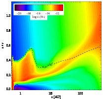
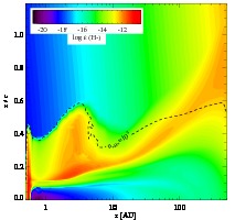
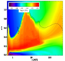
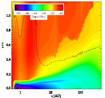
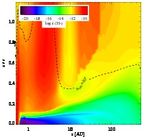
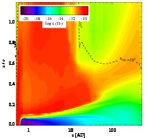
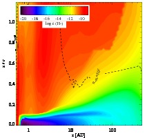
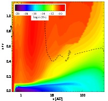
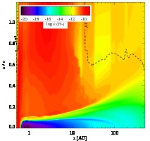
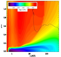
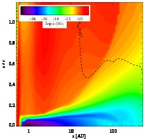
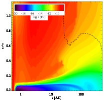
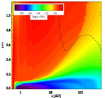
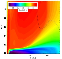
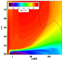
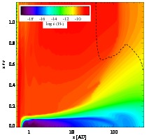
Figure 21: H^- abundances. FUV and X-ray fluxes are the same as Fig. 17.

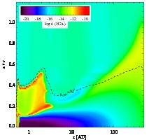
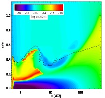
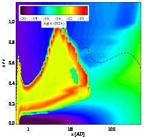
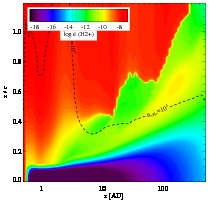
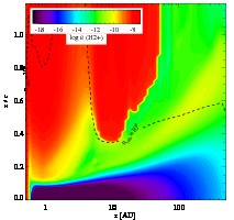
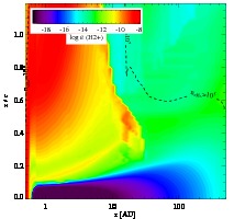
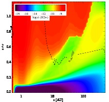
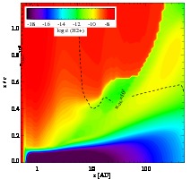
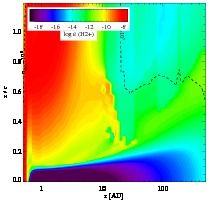
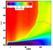
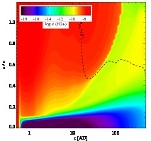
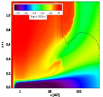
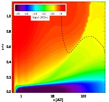
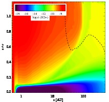
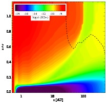
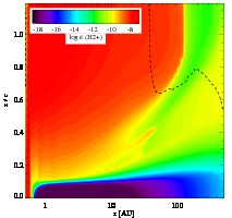
Figure 22: H${}_{2}^{+}$ abundances. FUV and X-ray fluxes are the same as Fig. 17.

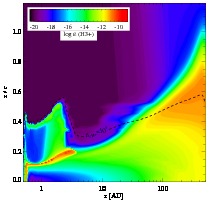
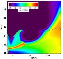
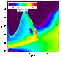
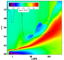
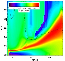
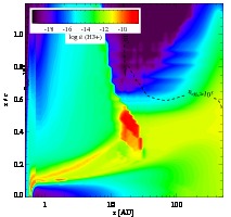
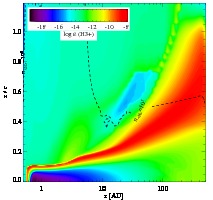
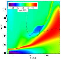
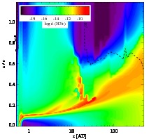
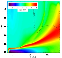
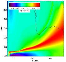
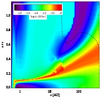
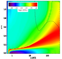
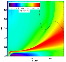
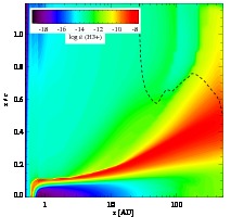
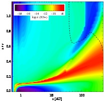
Figure 23: H${}_{3}^{+}$ abundances. FUV and X-ray fluxes are the same as Fig. 17.

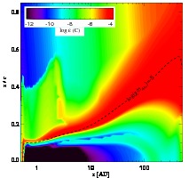
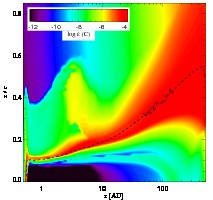
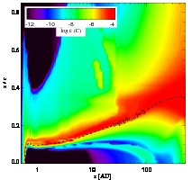
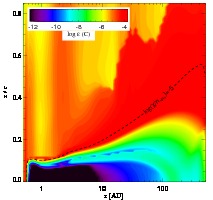
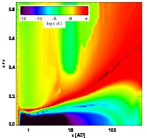
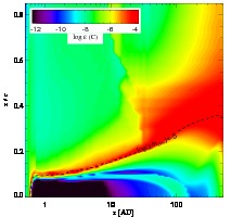
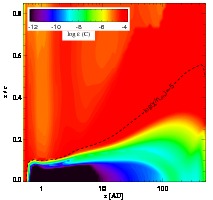
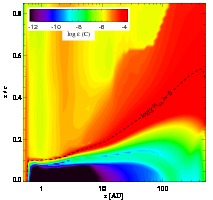
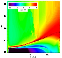
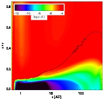
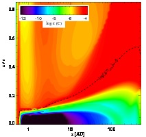
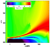
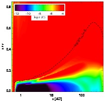
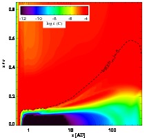
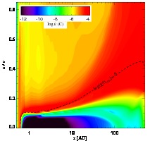
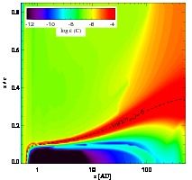
Figure 26: C abundances. FUV and X-ray fluxes are the same as Fig. 17.

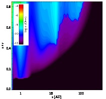
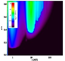
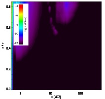
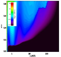
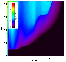
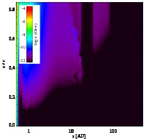
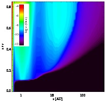
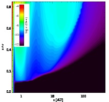
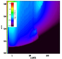
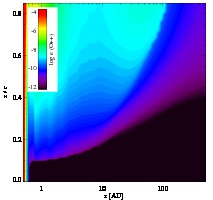
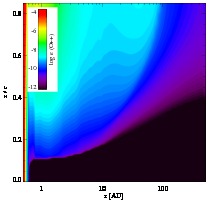
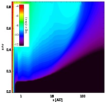
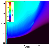
Figure 28: O²⁺ abundances. FUV and X-ray fluxes are the same as Fig. 17.

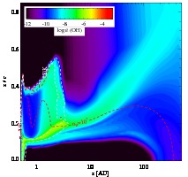
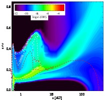
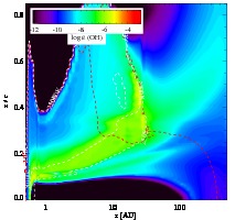
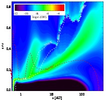
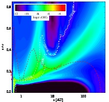
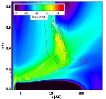
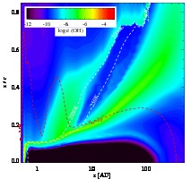
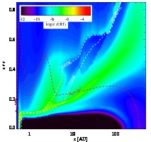
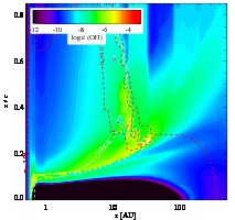
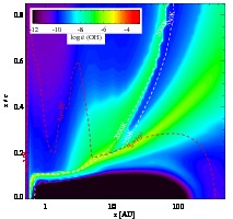
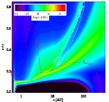
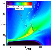
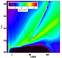
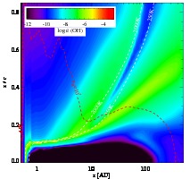
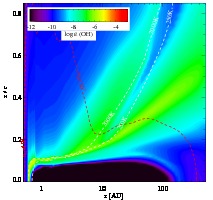
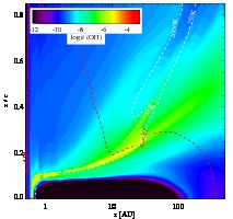
Figure 31: OH abundances. FUV and X-ray fluxes are the same as Fig. 17.

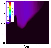
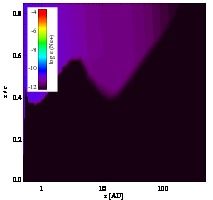
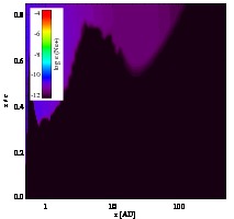
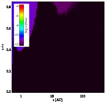
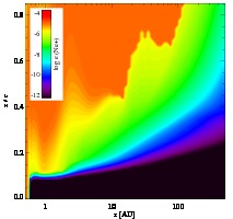
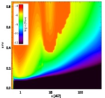
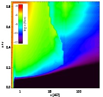
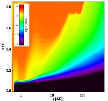
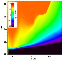
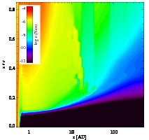
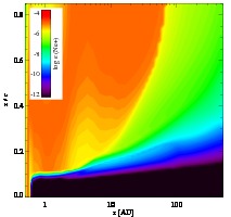
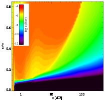
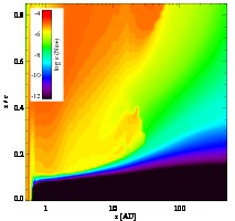
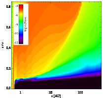
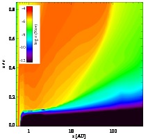
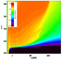
Figure 36: Ne⁺ abundances. FUV and X-ray fluxes are the same as Fig. 17.

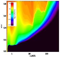
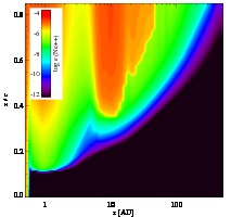
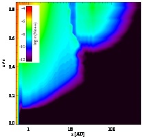
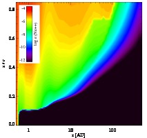
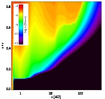
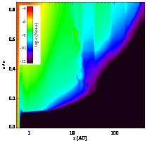
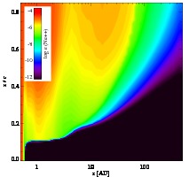
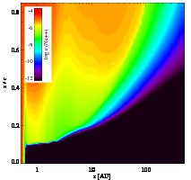
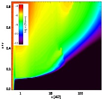
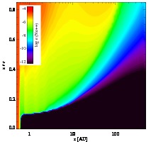
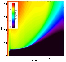
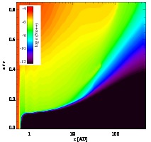
Figure 37: Ne²⁺ abundances. FUV and X-ray fluxes are the same as Fig. 17.

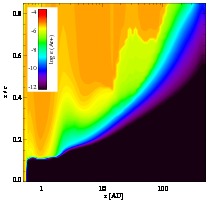
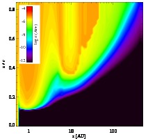
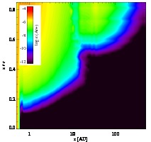
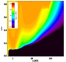
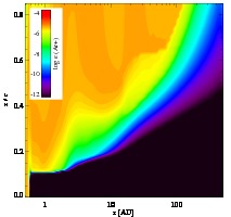
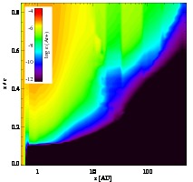
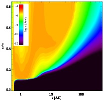
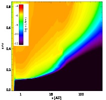
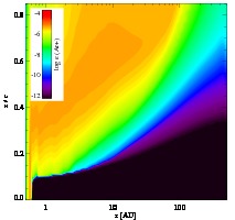
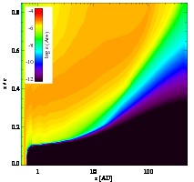
Figure 38: Ar⁺ abundances. FUV and X-ray fluxes are the same as Fig. 17.

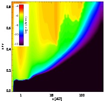
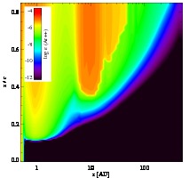
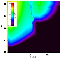
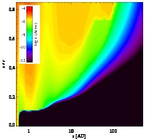
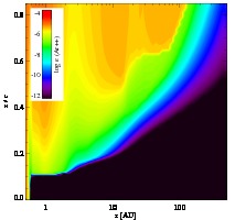
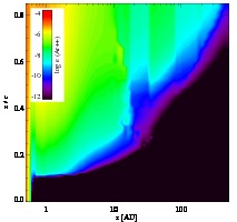
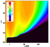
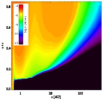
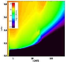
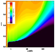
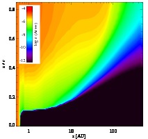
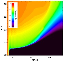
Figure 39: Ar²⁺ abundances. FUV and X-ray fluxes are the same as Fig. 17.

Figure 40: Radial column density distribution of C⁺. FUV and X-ray fluxes are the same as Fig. 17.

Figure 41: Radial column density distribution of Ne²⁺. FUV and X-ray fluxes are the same as Fig. 17.