Absorption Spectra of Astaxanthin Aggregates

Abstract

Carotenoids in hydrated polar solvents form aggregates characterized by dramatic changes in their absorption spectra with respect to monomers. Here we analyze absorption spectra of aggregates of the carotenoid astaxanthin in hydrated dimethylsulfoxide. Depending on water content, two types of aggregates were produced: H-aggregates with absorption maximum around 390 nm, and J-aggregates with red-shifted absorption band peaking at wavelengths >550 nm. The large shifts with respect to absorption maximum of monomeric astaxanthin (470-495 nm depending on solvent) are caused by excitonic interaction between aggregated molecules. We applied molecular dynamics simulations to elucidate structure of astaxanthin dimer in water, and the resulting structure was used as a basis for calculations of absorption spectra. Absorption spectra of astaxanthin aggregates in hydrated dimethylsulfoxide were calculated using molecular exciton model with the resonance interaction energy between astaxanthin monomers constrained by semi-empirical quantum chemical calculation. The intramolecular vibrations of astaxanthin are modeled by a line shape function corresponding to two characteristic C-C and C=C stretching modes with frequencies of 1150 cm^-1 and 1520 cm^-1. The solvent is represented by a spectral density of harmonic vibrations. The spectral changes at increasing concentrations of water were assigned to formation of aggregates with decreasing exposure of the astaxanthin hydrophobic chain to the solvent.

I Introduction

Carotenoids are a widespread group of natural pigments that attracted a lot of attention during the past decade due to their rich photophysics Polivka2004a-1 ; Ostroumov-2 ; Maiuri-3 ; Polivka-4 ; Kosumi-5 ; Gradinaru-6 . Their photophysical properties are important for their functions in photosynthetic organisms, where they act as key molecules in both light-harvesting and photoprotection Polivka-7 ; Ruban-8 . Based on a number of studies of monomeric carotenoids it is now a well-established fact that the strongly absorbing transition from the ground state responsible for the characteristic colors of carotenoids is not their lowest energy transition. Instead, at least one dark singlet state, denoted as the $S_{1}$ state, lies below the absorbing state which is denoted as $S_{2}$ state, accordingly Polivka2004a-1 . Moreover, recent results indicated that other dark states inaccessible from the ground state may be located within the $S_{1}$-$S_{2}$ energy gap Ostroumov-2 ; Maiuri-3 ; Polivka-4 ; Koyama-9 .

While the excited-state properties of monomeric carotenoids were studied to great details by various experimental and theoretical methods Polivka2004a-1 ; Ostroumov-2 ; Maiuri-3 ; Polivka-4 ; Kosumi-5 ; Gradinaru-6 ; Polivka-7 ; Ruban-8 ; Koyama-9 ; Starcke-10 ; Ghosh-11 ; Kleinschmidt-12 , spectroscopic properties of carotenoid aggregates, which are readily formed in hydrated polar solvents Simonyi-13 ; Billsten-14 ; Koepsel-15 ; Mori-16 ; Ruban-17 ; Giovannetti-18 , are much less understood. Two types of carotenoid aggregates can be distinguished according to their absorption spectra. The first type is associated with a large blue shift of the absorption spectrum of a monomeric carotenoid that is also accompanied by a loss of vibrational structure of the $S{}_{2}$ state. These aggregates are usually denoted as H-aggregates, in which the conjugated chains are closely packed oriented parallel to each other Simonyi-13 ; Spano-19 . The second aggregation type (J-aggregate) is characterized by a red-shift of the absorption spectrum, while the resolution of vibrational bands is mostly preserved. This aggregation (J-type) is likely a result of a head-to-tail organization of conjugated chains, forming a loose association of carotenoid molecules Simonyi-13 ; Spano-19 . Besides changes in absorption spectra, carotenoid aggregates also exhibit significant changes in circular dichroism (CD) Simonyi-13 , excited-state dynamics Billsten-14 , and Raman spectra Wang-20 ; Wang-21 .

Recent experimental studies showed that carotenoid aggregates may play a significant role in various natural and artificial systems. Carotenoids tend to aggregate when present in lipid bilayers, where they typically form H-type aggregates Sujak-22 ; Gruszecki-23 . However, it was recently shown that absorption changes consistent with J-type aggregation may occur in certain carotenoproteins Aspinall-24 ; chabera-25 . In artificial systems, H-aggregates are often formed when carotenoids are deposited on surfaces. Since assemblies consisting of carotenoid molecules attached to conducting or semiconducting materials hold promise to act as photoactive species in dye-sensitized solar cells Gao-26 ; Pan-27 ; Pan-28 ; Xiang-29 ; Wang-30 , understanding the effects of aggregation on the structure of excited states is an important factor in controlling the efficiency of such devices. Also, aggregation of carotenoids facilitates a homofission process Smith-31 , in which the $S_{1}$ state of carotenoid aggregate breaks down to form two triplets Wang-20 ; Wang-21 . When attached to an electron acceptor (e.g. TiO₂ semiconductor), this process promises to generate two electrons from a single absorbed photon, thus it is extremely attractive for the future design of devices aiming for conversion of solar energy to electricity.

Carotenoid astaxanthin, which is the subject of this study, is known mainly as the colorant of the lobster carapace where it is the only pigment of the carotenoprotein crustacyanin Cianci-32 . Upon binding to crustacyanin, absorption spectrum of astaxanthin undergoes a large red shift whose origin is still a matter of debate and excitonic interaction due to aggregation has been one of the suggested mechanisms of the red shift Wijk-33 . A few experimental studies of astaxanthin aggregation in hydrated solvents demonstrated that at ambient temperatures astaxanthin predominantly forms H-aggregates in hydrated acetone Mori-16 or methanol Koepsel-15 ; Giovannetti-18 . J-aggregates are generated and stabilized only upon heating up the system above 30 °C Giovannetti-18 . Yet, no theoretical studies aiming for explanation of aggregation-induced changes of absorption spectra of astaxanthin were carried out so far.

In this work, we explain absorption spectra of astaxanthin aggregates employing Frenkel exciton model for resonance interaction within astaxanthin aggregates, constrained by molecular dynamics simulations of an astaxanthin dimer. Two related models of astaxanthin aggregates are developed. For the purpose of calculating absorption spectra of astaxanthins, we introduce a molecular exciton model. In order to estimate one of the essential parameters of the exciton model, the resonance coupling, and in order to constrain its values for subsequent fitting, we use a more detailed, but still simplified, semi-empirical $\pi$-electron molecular orbital model of the astaxanthin. Excitonic model with explicit treatment of fast vibrational modes of carotenoids was used by Spano et al. Spano-19 to explain absorption and CD spectra of carotenoids. Here, the general approach is similar, although we do not consider the vibrational modes explicitly, but describe them by energy gap correlation function.

In Section II we discuss the preparation of the astaxanthin aggregates in different solutions. Section III, presents the lineshape method of calculation of absorption spectrum. The intramolecular vibrations of the astaxanthin are modeled by a two modes with frequencies $\omega_{vib}^{(1)}=1150$ cm^-1 and $\omega_{vib}^{(2)}=1520$ cm^-1 and the solvent is represented by a spectral density of harmonic vibrations (e.g. instantaneous normal modes). In Section IV we discuss the molecular exciton model, where the astaxanthin is represented by two electronic levels, (the ground state $|g\rangle$ and exited state $|e\rangle$) standing for the $S_{0}$ and the allowed $S_{2}$ states of the astaxanthin, respectively. We also discuss calculation of the absorption spectrum of the aggregates of astaxanthins based on such a model. The crucial parameter, which characterizes the aggregates assembled after the water is added into the solution, is the resonance coupling between the members of the aggregate. We perform molecular dynamics simulations in Section V to obtain an insight into the structure of the astaxanthin dimer in water. The average distance between the molecules in this case is used to qualitatively estimate the resonance coupling in Section VI. In Section VII we compare the spectra of different aggregates of astaxanthin and fit the experimental absorption spectra obtained under various solution conditions.

II Preparation of astaxanthin aggregates

Absorption spectra of astaxanthin monomers and aggregates in hydrated dimethylsulfoxide (DMSO) along with molecular structure of astaxanthin, are shown in Fig. 1. DMSO was chosen due to good solubility of astaxanthin in this solvent and also due to the large viscosity of DMSO which stabilizes aggregates. Also, as descried below, both types of aggregates can be readily formed in DMSO. Absorption spectrum of astaxanthin monomer in DMSO peaks at 20280 cm^-1 (493 nm). The $S_{0}$-$S_{2}$ transition of astaxanthin monomer does not exhibit any vibrational structure, a phenomenon characteristic of carotenoids having conjugated carbonyl groups Frank-34 ; Zigmantas-35 . Addition of water into the stock solutions of astaxanthin in DMSO changes absorption spectra significantly. All astaxanthin aggregates were prepared in a way that astaxanthin concentration, 20 $\mu$M, remains constant in all solvent/water mixtures.

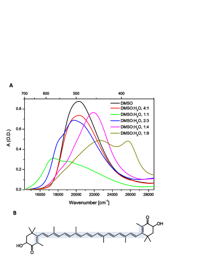
Figure 1: Part A: Absorption spectra of astaxanthin in pure DMSO and in various DMSO/water mixtures. In all samples, the concentration of astaxanthin is 20 (micro)M. Part B: Molecular structure of astaxanthin with the part of the $\pi-$conjugated system used for calculations marked in light blue.

In hydrated DMSO both J- and H-types of astaxanthin aggregates are readily formed. At DMSO:water ratio of 1:1, a clear band 17450 cm^-1 (573 nm) indicates that most of the astaxanthin molecules in solution formed J-aggregates. At increasing water concentration, J-aggregates transforms to H-aggregates as indicated by narrow absorption band at 25640 cm^-1 (390 nm). Thus, DMSO promotes formation of both types of aggregates with J-type generated only in rather narrow water concentration in agreement with earlier reports on astaxanthin Giovannetti-18 or zeaxanthin Billsten-14 in methanol. However, while in previous studies using methanol or acetone required higher initial concentrations of carotenoid to induce stable J-aggregates, in DMSO the J-aggregates are generated even at moderate concentration of 20 $\mu$M. Since we kept the concentration of astaxanthin constant during experiments, absorption spectra shown in Fig. 1 also demonstrate how the extinction coefficient of the $S_{0}$-$S_{2}$ transition changes upon aggregation. In both solvents, formation of aggregates is accompanied by significant decrease of extinction coefficient of both J- and H-aggregates.

III Calculation of Absorption Spectrum

In order to characterize absorption spectra of astaxanthin aggregates, we apply a line shape model based on second cumulant expansion of the electron-phonon coupling. In contrast to recently reported vibronic exciton approach aiming to explain absorption and CD spectra of aggregates of another carotenoid, lutein Spano-19 , we do not treat vibrational modes of the carotenoid explicitly. In the case of a carotenoid monomer, the two approaches would lead to the same results (second cumulant expansion is exact for calculation of absorption spectra of harmonic systems Doll2008a ). The reduction to a purely electronic exciton approach, which is very successful in describing chlorophyll based aggregates Cho2005a , simplifies the treatment of the system significantly. It is also motivated by the lack of detailed vibrational structure in astaxanthin and by only a small perturbation of the vibrational band structure upon aggregation reported for other carotenoids Wang2012

The astaxanthin molecule in solution can be represented by the following Hamiltonian

$$H_{{\rm car}}=(\epsilon_{g}+T+V_{g})|g\rangle\langle g|+(\epsilon_{e}+T+V_{e})|e\rangle\langle e|,$$ (1)

where the states $|g\rangle$ and $|e\rangle$ were introduced in Section I, $\epsilon_{g}$ and $\epsilon_{e}$ are the ground and excited state electronic energies, $T$ represents the kinetic energy operator of the intramolecular nuclear modes of the carotenoid and the kinetic energy of the solvent DOF, and $V_{g}$ and $V_{e}$ represent the potential energy surfaces of these DOF in the electronic ground and excited states, respectively. The Hamiltonian, Eq. (1), can be split into the usual system (S), bath (B) and interaction (I) parts as follows

$$H_{{\rm car}}=\underbrace{T+V_{g}}_{H_{B}}+\underbrace{\epsilon_{g}|g\rangle\langle g|+[\epsilon_{e}+\langle V_{e}-V_{g}\rangle_{eq}]|e\rangle\langle e|}_{H_{S}}$$

$$+\underbrace{\Delta V|e\rangle\langle e|}_{H_{I}}.$$ (2)

In the interaction Hamiltonian $H_{I}$ we introduced so-called energy gap operator

$$\Delta V=V_{e}-V_{g}-\langle V_{e}-V_{g}\rangle_{eq},$$ (3)

where $\langle V_{e}-V_{g}\rangle_{{\rm eq}}={\rm tr}\{(V_{e}-V_{g})W_{{\rm eq}}\}$ is the equilibrium expectation value of the difference between the excited state and the ground state nuclear PES.

To describe spectroscopy, let us introduce the light-matter interaction Hamiltonian in the semiclassical dipole approximation, i.e.

$$H_{E}(t)=-\bm{\mu}\cdot\bm{E}(t),$$ (4)

where the dipole moment operator reads

$$\bm{\mu}=\bm{d}|g\rangle\langle e|+\bm{d}^{*}|e\rangle\langle g|,$$ (5)

with $\bm{d}$ independent of the solvent and intramolecular carotenoid DOF (Condon approximation). The absorption coefficient can then be expressed in terms of linear response function $S^{(1)}(t)$ as MukamelBook

$$\alpha(\omega)=\frac{\omega}{n(\omega)}{\rm Re}\int\limits_{0}^{\infty}d\omega\ S^{(1)}(t)e^{i\omega t}.$$ (6)

For a two-level system interacting with harmonic oscillators, exact expression for the linear response function can written down in terms of the so-called line shape function

$$g(t)=\frac{1}{\hbar^{2}}\int\limits_{0}^{t}d\tau\int\limits_{0}^{\tau}d\tau^{\prime}C(\tau^{\prime}),$$ (7)

where $C(t)$ is so-called bath or energy gap correlation function

$$C(t)={\rm tr}\{e^{\frac{i}{\hbar}H_{B}t}\Delta Ve^{-\frac{i}{\hbar}H_{B}t}\Delta V\ W_{{\rm eq}}\}.$$ (8)

Here, $W_{{\rm eq}}$ is the equilibrium density matrix of the intramolecular and solvent DOF. The first order response now reads as

$$S^{(1)}(t)=\frac{i}{3}\Theta(t)|d|^{2}e^{-g(t)-i\omega_{eg}t}.$$ (9)

The prefactor $\frac{1}{3}$ results from the averaging of the response function over an isotropic distribution of the dipole moment vectors of the molecule in space. By prescribing the correlation function $C(t)$ in a form of two independent contributions

$$C(t)=C_{{\rm vib}}(t)+C_{{\rm solvent}}(t),$$ (10)

where the contribution of intramolecular vibrations

$$C_{{\rm vib}}(t)=\lambda_{{\rm vib}}\Big{(}\frac{2k_{B}T}{\hbar}\cos(\omega_{{\rm vib}}t)$$

$$-i\omega_{{\rm vib}}\sin(\omega_{{\rm vib}}t)\Big{)}e^{-\Gamma_{{\rm vib}}t/2},$$ (11)

and the contribution of solvent reads as

$$C_{{\rm solvent}}(t)=\lambda_{{\rm solv}}\left(\frac{2k_{B}T}{\hbar}-i\Gamma\right)e^{-\Gamma t},$$ (12)

we completely specify the absorption spectrum of the monomer. Details of the model correlation functions Eqs. (11) and (12) can be found in the Ref. MukamelBook .

The correlation function, Eq. (8), enables us to describe another important contribution to the absorption spectrum, so-called static disorder or inhomogeneous broadening. Provided that there is a certain distribution of transition energies $\hbar\omega_{eg}$ such that it is characterized by a constant energy gap correlation function $C_{{\rm dis.}}(t)=\Delta^{2}$, this could be easily incorporated into the absorption spectrum formula, Eq. (6), which now reads

$$\alpha(\omega)=\frac{\omega|d|^{2}}{3n(\omega)}{\rm Im}\int\limits_{0}^{\infty}d\omega\ e^{-g(t)-\frac{\Delta^{2}}{2\hbar^{2}}t^{2}-i(\omega_{eg}-\omega)t}.$$ (13)

Instead of Eq. (13), one can alternatively use explicit drawing of the energy gap value out of a Gaussian distribution with the width $\Delta^{2}$. For a monomer, both approaches are equivalent. For aggregate, the line-shape function depends on the aggregate structure, and the simulation of disorder has to be preformed explicitly.

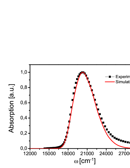
Figure 2: Experimental (red) and calculated (black) absorption spectrum of a monomer astaxanthin in DMSO. The parameters of calculation are: transition frequency $\omega_{eg}=20700$ cm^-1, vibrational frequencies $\omega_{{\rm vib}}^{(1)}=1520$ cm^-1, and $\omega_{{\rm vib}}^{(2)}=1150$ cm^-1, reorganization energies of the vibrations $\lambda_{{\rm vib}}^{(1)}=1220$ cm^-1, and $\lambda_{{\rm vib}}^{(2)}=250$ cm^-1, damping time of the vibrations $\tau_{{\rm vib}}^{(1,2)}=\frac{1}{\Gamma_{{\rm vib}}}=1$ ps, solvent reorganization energy $\lambda_{{\rm solv}}=550$ cm^-1, solvent correlation time $\tau_{c}=100$ fs.

IV Excitonic Model

When aggregates are formed in the solution, astaxanthin molecules start to interact with each other. We will use the subscript $n$ and the superscript $(n)$ to distinguish individual molecules of the aggregate in this section. The total Hamiltonian reads

$$H=\sum_{n=1}^{N}H_{{\rm car}}^{(n)}+H_{{\rm int}},$$ (14)

where $H_{{\rm int}}$ represents all possible interaction terms that follow from quantum chemistry. Electronic states of the aggregates can be expressed using the basis composed of excitations of individual monomers. The aggregate is in the ground state when all the molecules in the aggregate are in the ground state. Thus we can write

$$|G\rangle\equiv\prod_{n=1}^{N}|g_{n}\rangle,$$ (15)

where $|g_{n}\rangle$ is the ground state of the n^th astaxanthin. The excited states of the aggregate in the spectral region around the $S_{2}$ band of the monomeric astaxanthin are formed from single excitation states

$$|E_{k}\rangle=\prod_{n=1}^{k-1}|g_{n}\rangle|e_{k}\rangle\prod_{m=k+1}^{N}|g_{m}\rangle,$$ (16)

where $|e_{k}\rangle$ is the excited $S_{2}$ state of the k^th astaxanthin in the aggregate.

Expressed in these states, the aggregate Hamiltonian reads

$$H=H_{B}+\sum_{n}(\tilde{\epsilon}_{n}+\Delta V^{(n)})|E_{n}\rangle\langle E_{n}|$$

$$+\sum_{m\neq n}J_{mn}|E_{m}\rangle\langle E_{n}|,$$ (17)

where the ground state energy of the aggregate $\epsilon_{g}$ is set to zero, $\tilde{\epsilon}_{n}=\hbar\omega_{eg}^{(n)}$ is the excited state energy of the n^th astaxanthin ($\tilde{\epsilon}_{n}=\epsilon_{e}+{\rm tr}_{{\rm bath}}\{(V_{e}^{(n)}-V_{g}^{(n)})W_{eq}\}$) and $J_{nm}$ is the electrostatic coupling between two astaxanthins

$$J_{nm}={\rm tr}_{{\rm bath}}\{\langle E_{n}|H_{int}|E_{m}\rangle W_{eq}\}.$$ (18)

The electronic eigenstates of the Hamiltonian, Eq. (17), can be found by the diagonalization of its purely electronic part (i.e. ignoring $\Delta V^{(n)}$ and $H_{B}$ in Eq. (17)). The new excited eigenstates and their energies will be denoted $|\bar{E}_{n}\rangle$ and $\bar{\epsilon}_{n}$, respectively. The total Hamiltonian now reads

$$H=H_{B}+\sum_{n}(\bar{\epsilon}_{n}+\Delta\bar{V}_{nn})|\bar{E}_{n}\rangle\langle\bar{E}_{n}|$$

$$+\sum_{m\neq n}\Delta\bar{V}_{mn}|\bar{E}_{m}\rangle\langle\bar{E}_{n}|.$$ (19)

The last term represents energy transfer between the electronic eigenstates of the aggregate, the effects of which lead to broadening of the absorption spectra. We will ignore these effects in further discussion and assume them to be smaller than the effects of broadening due to pure dephasing (the diagonal term $\Delta\bar{V}_{nn}$) and the disorder. The pure dephasing terms read as

$$\Delta\bar{V}_{nn}=\sum_{k}|\langle\bar{E}_{n}|E_{k}\rangle|^{2}\Delta V^{(k)}.$$ (20)

The delocalized eigenstates $|\bar{E}_{n}\rangle$ are usually termed molecular excitons ValkunasBook . Thus we arrive at a situation which is similar to calculation of the absorption spectrum of the monomer, Eq. (13), except of the number of involved states which is equal to the number of members of the aggregate. We thus have

$$\alpha(\omega)=\frac{\omega}{3n(\omega)}\langle\sum_{n}|d_{n}|^{2}{\rm Im}\int\limits_{0}^{\infty}d\omega\ e^{-g_{nn}(t)-i(\omega_{ng}-\omega)t}\rangle_{diss},$$ (21)

where $\langle\dots\rangle_{diss}$ denotes explicit averaging over energy gap disorder, $d_{n}$ are the transition dipole moments of the $n^{th}$ eigenstate, and $g_{nn}(t)$ is the lineshape function corresponding to the energy gap operator $\Delta\bar{V}_{nn}$ in the Hamiltonian Eq. (19). Assuming that the bath fluctuations on different molecules are the same, but are not correlated, we can write for the line shape functions

$$g_{nn}(t)=\sum_{k}|\langle\bar{E}_{n}|E_{k}\rangle|^{4}g(t),$$ (22)

where $g(t)$ is the lineshape function of a monomeric molecule.

V Molecular Dynamics Simulation

In order to obtain parameters for calculation of excitonic interaction, aggregation of astaxanthin dimer in aqueous solution was studied by means of classical molecular dynamics (MD) simulations with non-polarizable force fields. The simulated system consisted of two astaxanthin molecules and 2700 water molecules forming a slab of liquid in the center of the simulation box, with two water/vapor interfaces perpendicular to the z axis. The x, y and z-dimensions of the rectangular simulation box were set to 50.0, 50.0 and 100.0 Å, respectively with periodic boundary conditions in all three dimensions. The astaxanthin carotenoid molecule was modeled by using the general Amber force field (GAFF) Wang-36 and water molecules were modeled by using SPC/E model Berendsen-37 . To obtain partial charges of astaxanthin molecule, ab initio geometry optimization of single astaxanthin molecule was performed using the Gaussian 03 package gaussian03-38 by employing the density functional theory B3LYP/cc-pVT. After the optimization by ab initio calculations, restricted electrostatic potential (RESP) procedure was applied using Antechamber program Wang-39 , which is implemented in the Amber program package amber8-40 for obtaining the atomic partial charges. For preparation of the initial configuration, two astaxanthin molecules with distance of larger than 10 Å were solvated in water box, which was followed by energy minimization for a few thousands steps. The system was then equilibrated for 2 ns followed by a 5 ns production run. The simulation was carried out in the NVT ensemble at 300 K, and temperature was controlled by the Berendsen thermostat Berendsen-41 . Equations of motion were integrated using the Leapfrog algorithm with the time step of 1 fs. The non-bonding interactions were cut at distance of 12.0 Å, and long-range electrostatic interactions were treated by the Particle Mesh Ewald procedure Daren-42 ; Essmann-43 . All bonds involving hydrogen atoms were constrained using the SHAKE algorithm Ryckaert-44 and a trajectory was constructed by sampling the coordinates at each 5 ps for further analysis such as distance between conjugated chains and head groups. All MD simulations were performed by employing Amber85 program package, and VMD program was used for visualizations and preparation of snapshots and distances Humphrey-45 . Fig. 3 shows typical snapshot from MD simulation which shows the aggregation taking place when astaxanthin molecules solvate in the aqueous solutions. The structure of astaxanthin dimer is stabilized within first few ps, which was revealed by analyzing the trajectory from MD simulation. The conjugated chains of two astaxanthin molecules have in average the distance of 4.1 Å though the head groups can have even closer distances during the MD simulation.

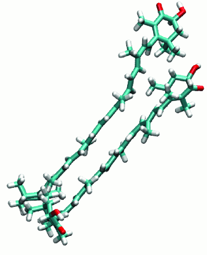
Figure 3: Structure of astaxanthin dimer resulting from molecular dynamics simulations. Carbon atoms are shown in blue, hydrogens are white and oxygens red.

VI Resonance Coupling between Carotenoid Molecules

Within the usual excitonic model one could calculate resonance coupling between two molecules in dipole-dipole approximation. Transition dipole moment vector and mutual positions of the molecules are parameters of the model. This approximation is applicable to well spaced compact molecules, such as chlorophylls in photosynthetic antennae (i.e. in proteins), but fails for chain-like molecules such as astaxanthins in solution. Obviously, the distance between two astaxanthins can be much smaller than the extent of the molecule, in which case dipole-dipole approximation breaks down. In order to estimate the coupling between astaxanthins, we need to use quantum chemical packages, or, as we do here, to construct a phenomenological model carotenoid with a qualitative description of the molecular states. We aim at a qualitative theory of coupling, which allows us to make claims beyond the validity of the dipole-dipole approximation.

The $S_{2}$ state of a carotenoid originates from the excitation of the conjugated $\pi$-electronic system. Therefore, we consider only the delocalized $\pi$-electrons, and we calculate its wavefunction using an Hückel type semi-empirical method. Our model carotenoid is made of carbon atoms with bond length $1.4$ Å and with positions chosen in such way, that all bonding angles are 120°. The structure is depicted on Fig. 1. We describe the $\pi$-electron p-orbital wavefunctions by the STO-3G basis of atomic orbitals Szabo1996a .

Inspired by the extended Hückel method (EHM) Hoffmann1963 , we define the Hückel Hamiltonian in the form

$$\langle\phi_{\mu}|H^{Huckel}|\phi_{\nu}\rangle=H_{\mu\nu}^{Huckel}=\delta_{\mu\nu}\alpha+(S_{\mu\nu}-\delta_{\mu\nu})\beta,$$ (23)

where $S_{\mu\nu}\equiv\langle\phi_{\mu}|\phi_{\nu}\rangle$ are overlap integrals of the atomic orbitals $|\phi_{\mu}\rangle$ and $\alpha$, $\beta$ are parameters of the method constructed from valence state ionization potentials Hoffmann1963 . By solving eigenvalue problem in a form

$$\sum_{\nu}H_{\mu\nu}^{Huckel}c_{\nu i}=\varepsilon_{i}\sum_{\nu}S_{\mu\nu}\,c_{\nu i},\;$$ (24)

we obtain the expansion coefficients $c_{i}$ of the molecular orbitals in the basis of the atomic orbitals. Eq. (24) can be rewritten as

$$\alpha^{\prime}\sum_{\nu}\delta_{\mu\nu}c_{\nu i}=\varepsilon{}_{i}^{\prime}\sum_{\nu}S_{\mu\nu}c_{\nu i}$$ (25)

with $\alpha^{\prime}=\alpha-\beta$ and $\varepsilon{}_{i}^{\prime}=\varepsilon{}_{i}-\beta$. We fit the parameter $\alpha^{\prime}$ to reproduce values of HOMO-LUMO transition energies of several polyenes of a different length reported in Ref. Smith2004 . Because we are interested in only in the energy difference, the particular value of the parameter $\beta$ is irrelevant, and we may work with just $\alpha^{\prime}$. Unlike in the original EHM, this value does not have a direct physical interpretation. The comparison with polyens yields

$$\alpha^{\prime}=66.48\;\mathrm{eV}.$$ (26)

Using the obtained molecular orbitals, we calculate the HOMO-LUMO energy gap and the related transition dipole moment in a standard manner. We get

$$\begin{array}[]{c}\Delta E^{HOMO-LUMO}=20742\;{\rm cm}^{-1},\\ |\mathbf{d}_{trans.}^{HOMO-LUMO}|=28.6\;\mathrm{D\;.}\end{array}$$ (27)

In order to calculate the resonance coupling between two astaxanthins, we evaluate the corresponding matrix element of the electrostatic interaction Hamiltonian Madjet2006

$$V_{ab,a^{\prime}b^{\prime}}=\int d\mathbf{r}_{1}\dots d\mathbf{r}_{N}\int d\bar{\mathbf{r}}_{1}\dots d\bar{\mathbf{r}}_{N}$$

$$\Psi_{a}^{*}(\mathbf{r}_{1},\dots,\mathbf{r}_{N})\Psi_{b}^{*}(\mathbf{\bar{r}}_{1},\dots,\mathbf{\bar{r}}_{N})$$

$$\times\Bigg{\{}\sum_{i,j}\frac{1}{|\mathbf{r}_{i}-\mathbf{\bar{r}}_{j}|}-\sum_{i,J}\frac{Z_{J}}{|\mathbf{r}_{i}-\mathbf{\bar{R}}_{J}|}-\sum_{I,j}\frac{Z_{I}}{|\mathbf{R}_{I}-\mathbf{\bar{r}}_{j}|}$$

$$+\sum_{I,J}\frac{Z_{I}Z_{J}}{|\mathbf{R}_{I}-\mathbf{\bar{R}}_{J}|}\Bigg{\}}\Psi_{a^{\prime}}(\mathbf{r}_{1},\dots,\mathbf{r}_{N})\Psi_{b^{\prime}}(\mathbf{\bar{r}}_{1},\dots,\mathbf{\bar{r}}_{N})\;.$$ (28)

Here, $N$ is the number of all electrons of given molecule, $Z_{I}$ are the nuclear charges in units of the elementary charge, $\mathbf{r}_{i}$ and $\mathbf{\bar{r}}_{i}$ are coordinates of electrons of astaxanthin 1 and 2, $\mathbf{R}_{I}$ and $\mathbf{\bar{R}}_{I}$ are coordinates of nuclei of astaxanthin 1 and 2 and $\Psi_{a}(\mathbf{r}_{1},\dots,\mathbf{r}_{N})$, $\Psi_{b}(\mathbf{\bar{r}}_{1},\dots,\mathbf{\bar{r}}_{N})$ are complete electronic wavefunctions of astaxanthin 1 and astaxanthin 2 respectively. They are constructed as Slater determinants from atomic orbitals. Overlaps between atomic orbitals of different astaxanthins are neglected. Contributions of particular terms of Hamiltonian, Eq. (28), can be found by using the Slater-Condon rules for matrix elements Szabo1996a .

VII Absorption Spectra of Astaxanthin Aggregates

Molecular dynamics simulations show that in water carotenoids tend to minimize the exposure of their hydrophobic chain to the solvent. Thus a parallel dimer (see Figs. 3 and 4) is a possible arrangement. The dipole-dipole coupling formula predicts a positive value $J$ of the resonance coupling. Excitonic model predicts in such a dimer existence of two exited states, which have a form of a symmetric and anti-symmetric linear combinations of the $S_{2}$ excited states of individual astaxanthins. For the parallel dimer arrangement, optical excitation of the energetically higher state is allowed, whereas the lower lying state is dark. Thus one expects a blue shift of the absorption spectrum upon aggregation.

However, in a mixture of DMSO and water, at the percentage of water of $50-60$ we observe a red shift (see Fig. 1). Such a shift requires negative value of the resonance coupling. Dipole-dipole coupling formula results in negative coupling for a “serial” dimer (see Fig. 4) where the centers of the astaxanthins are shifted by a sufficient distance $X$. As we discussed above, dipole-dipole coupling is not a reliable approximation for astaxanthins, and we therefore performed a calculation for different values of $X=0,\dots,30$ Å and $R=4.1$ Å (the value predicted by MD simulations in Section V) with our semi-empirical method. The resulting values of coupling are presented in Fig. 5 and the comparison of the two predictions is made in the inset. Both results coincide for large distances $R$ and $X$ where dipole approximation holds. One can immediately notice that dipole-dipole formula grossly overestimates the positive coupling for $X=0$, it predicts a rapid switch to negative values of $J$ (at $X=2.9$ Å) and even for larger $X$ it overestimates the magnitude of the negative coupling. Our Hückel-type calculation, on the other hand, predicts moderate values of the resonance coupling (between $-1500$ and $3000$ cm^-1), and the switch from positive to negative values occuring at larger $X$, roughly when $X$ is comparable with the half length of the astaxanthin conjugated chain. Since our calculations of the resonance coupling are too simple to aim at quantitative results, we will use the parameter $J$ for selected structures as a fitting parameter in the next section. We also constrain the resonance coupling to values up to few thousands of cm^-1.

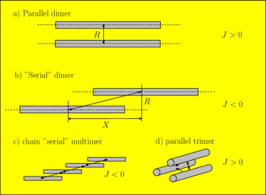
Figure 4: Characteristic structures of the astaxanthin dimers and aggregates used for calculation of absorption spectra. Part a) Parallel dimer and similar slightly shifted arrangements are characterized by $J>0$. Part b) The “serial” dimer with large shift $X$ is characterized by $J<0$. Part c) Larger aggregates of the “serial” character can have a form of chains. Part d) The parallel dimer can form stacks or more compact structures such as a trimer with equal distance between the conjugated chains of the three molecules.

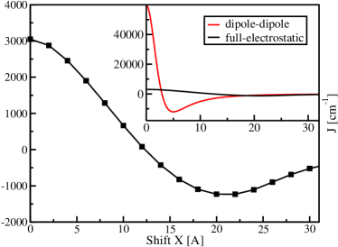
Figure 5: Dependence of the resonance coupling on the mutual shift $X$ (see Fig. 4) of the astaxanthin molecules .

To analyze the absorption spectra of astaxanthin in DMSO with varying percentage of water, we calculated spectra of the two representative mutual configurations of astaxanthin molecules, namely those with positive and negative resonance coupling energy $J$. We start with a simple idea that with increasing percentage of water in the solutions, it will become energetically advantageous for the molecules to minimize the surface of their hydrophobic chains exposed to water. With small amount of water, the free energy profile will be rather flat and we might preferentially find the molecules in the arrangement similar to that one of the “serial” dimer (see Fig. 4). With increasing amount of water a strict parallel dimer arrangement will be more and more preferred.

It is in no way plausible that one could reproduce the absorption spectrum by composing it from a small number discrete structures, e.g. dimers and trimers of particular value of coupling $J$. It is more likely that there exists a smooth distribution of structures depending on the particular interactions between molecules and the solvent at a given concentration of water. This would result in a distribution of values of the coupling $J$. A direct simulation of the disordered structure of aggregates requires some prescription of the probability of various configuration. In the absence of a physical model supporting the distribution, one might attempt an effective approach, where the fluctuation of the structure would be simulated by fluctuations of the transition energies of the carotenoids (disorder parameter $\Delta$) in several selected structures. If successful, it could provide guidance in constructing a more detailed model of aggregation which would take into account the thermodynamics of the process.

The exciton model is not able to account for the reduced extinction coefficient of the aggregates. The total calculated extinction coefficient of the aggregates would thus be overestimated. As a result, one cannot expect to deduce actual concentrations of the aggregates from our model, because the transition dipole moment of an aggregate is reduced by an unknown factor. In order to fit the experimental spectra, we will therefore calculate normalized absorption spectra $\alpha_{1}(\omega)$, $\alpha_{2}(\omega,J_{2})$, $\alpha(\omega,J_{3})$,$\dots$ for monomer, dimer, trimer and larger aggregates with some values $J$ of the resonance coupling. We will then combine them to get the total normalized absorption spectrum $\alpha(\omega)$ as

$$\alpha(\omega)=\frac{1}{{\cal N}}\sum_{n=1}^{K}a_{k}\alpha_{k}(\omega,J_{k}),$$ (29)

where ${\cal N}$ is a normalization constant. This will give us an qualitative picture of the ratio of various aggregates in the mixture,

The values of $J$ and the selected structures where chosen according to the features observed in the astaxanthin spectra at 50 % and 90 % of water (see Fig. 1A) while taking into account qualitative results of the molecular orbital simulations. Such a procedure cannot lead to unique results, but still seriously constrains the composition of the aggregate spectra, as demonstrated below.

VIII Discussion

VIII.1 J-Aggregate Spectrum

Let us first analyze the spectra measured at $50$ % of water. The experimental spectrum shows a significant red shift by $\approx 2800$ cm^-1. This is consistent with formation of J-aggregates ($J<0$) i.e. with the “serial” dimer and larger aggregates of the similar form. Combination of the monomeric spectrum with a spectrum of the dimer ($J=-2500$ cm^-1) leads to the spectrum with characteristic shoulder. Adding small portions of trimers, tetramers and larger aggregates up-to six members leads to a good fit of the experimental spectrum (black dashed curve in Fig. 6) starting from $16000$ cm^-1, with slightly insufficient absorption for frequencies larger than $20000$ cm^-1. The spectral region between $14000$ cm^-1 and $16000$ ^-1 probably contains aggregates with even more members than six. By adding the parallel dimer spectrum (taken from the fit of the spectra at 90 % of water, see below) we obtain far better fit for the frequencies above $20000$ cm^-1 confirming the presence of some parallel H-aggregate type dimers already at $50$ % of water.

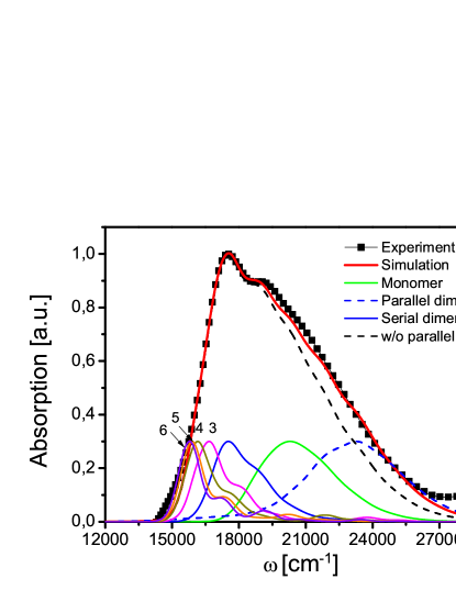
Figure 6: Absorption spectrum of a mixture of astaxanthin aggregates at 50 % of water. Theoretical spectrum is composed of aggregates up to six members with $J<0$ (parallel dimer) and of a sizable amount of parallel dimers with $J>0$ (see Tab. 1). The spectra of various aggregates are all normalized for their maximum equal to 0.3.

The parameters of the fit are summarized in Tab. 1. The fit is composed of absorption spectra of small aggregates whose constituents have the parameters same as the monomer in Fig. 2 . The influence of the trimer and larger aggregate spectra on the total spectrum is small and it was not possible to make conclusions on the magnitude of the disorder in them. We leave their disorder the same as in the monomer.

Nr. of members	$\Delta$ [cm-1]	$J$ [cm-1]	$\frac{a_{n}}{{\cal N}}$
1	800	-	0.50
2	800	-2500	0.75
3	800	-2500	0.28
4	800	-2500	0.09
5	800	-2500	0.03
6	800	-2500	0.02
2	2400	2100	0.21

Table 1: Parameters of the fit in Fig. 6. First column represents the number of monomers in an aggregate. The transition energies $\hbar\omega_{eg}$ are those of the monomer in Fig. 2 (parameters in the text) with disorder parameter $\Delta$ and nearest neighbor coupling $J$. The sum spectrum is composed of the normalized spectra of various aggregates according to Eq. (29) with coefficients $a_{n}$. The last row is the parallel dimer from Tab. 2.

VIII.2 H-Aggregate Spectrum

At the concentration of water equal to 90 %, we can assume the formation of parallel dimers and possibly larger aggregates of similar structure. Positive resonance coupling is suggested by the blue shift of the spectrum with respect to the spectrum of the monomer. The line shape can be fitted by a mixture of monomers, dimers and trimers of the parallel type, and a small contribution of the “serial” dimers. The parallel dimer has to have a significantly larger disorder than the monomer, suggesting the existence of coupling disorder or some deformation of the chain . The trimer contribution cannot be explained by simple stacking of the monomers. This would result in a nearest neighbor coupling and a second nearest neighbor coupling significantly reduced, and correspondingly in an insufficient shift of the trimeric peak. We have to rather assume an increased excitonic coupling which acts among all three molecules of the aggregate. This is consistent with all three molecules touching by their conjugated chains (see Fig. 4D) and a compactification of the aggregate (molecules are closer to each other than in the dimer). As an alternative to this fit, one could try to explain the most blue peak of the experimental H-aggregate spectrum of astaxanthin (Fig. 7) by a dimer with large resonance coupling. This coupling would, however, have to be almost an order of magnitude larger than the one calculated by our semi-empirical method. Assuming a compactified trimer returns the required values of resonance coupling into a reasonable parameter region.

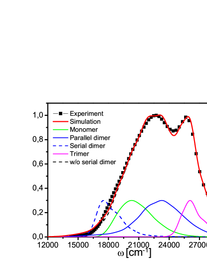
Figure 7: Absorption spectrum of a mixture of astaxanthin aggregates at 90 % of water. The spectrum is composed of mono-, di- and trimers with $J>0$ (parallel dimer) and of a small amount of “serial” dimers with $J<0$ (see Tab. 2). The spectra of various aggregates are all normalized for their maximum equal to 0.3.

Nr. of members	$\Delta$ [cm-1]	$J$ [cm-1]	$\frac{a_{n}}{{\cal N}}$
1	800	-	0.36
2	2400	2100	0.87
3	1200	2750	0.60
2	800	-2500	0.06

Table 2: Parameters of the fit in Fig. 2 First column represents the number of monomers in an aggregate. The transition energies $\hbar\omega_{eg}$ are those of the monomer in Fig. 2 (parameters in the text) with disorder parameter $\Delta$. In case of a dimer, $J$ represents the coupling between the two monomers, for trimer $J$ is the coupling of a monomer to other two monomers. The sum spectrum is composed of the normalized spectra of parallel mono-, di- and trimers and “serial” dimer. The sum spectrum is composed of the normalized aggregate spectra according to Eq. (29) with coefficients $a_{n}$. The last row is the “serial” dimer from Tab. 1.

In both investigated absorption spectra (Figs. 6 and 7) we can see several distinct excitonic features. The most significant feature is the spectral shift of the bands. However, the line shapes also bear signatures of band narrowing, evident e.g in the appearance of the vibrational shoulder in the dimer spectrum at $50$ % of water, or in the narrow line shape of the trimers at $90$ % of water. Both these shapes determine the most obvious features of the aggregate spectra.

IX Conclusions

We have measured and analyzed absorption spectra of aggregates of the carotenoid astaxanthin in hydrated dimethylsulfoxide. We have demonstrated that these absorption spectra can be explained quantitatively as a sum of spectra of small aggregates. Phenomenological excitonic model of resonance interaction between $\pi-$conjugated chains of astaxanthin molecules was constrained by semi-empirical calculations. The observed spectral shifts were assigned to formation of J-type and H-type aggregates and their changing ratio under different concentration of water. Fitting experimental absorption spectra lead to a qualitative estimation of ratio of aggregates of various types in the sample at 50 % and 90 % of water in dimethylsolfoxide. With increased percentage of water in the solvent, the proportion of compact aggregates with a decreasing surface area exposed to the solvent is growing. Based on absorption spectra, it is not possible to exclude that different aggregate configurations result in the same observed features. The ease with which the spectra can be explained by the spectra of small aggregates, however, provides a relatively high degree of confidence in our results.

- (1) T. Polívka and V. Sundström, Chem. Rev. 104, 2021 (2004).
- (2) E. Ostroumov, M. Muller, C. Marian, M. Kleinschmidt, and A. Holzwarth, Phys. Rev. Lett. 103, 108302 (2009).
- (3) M. Maiuri, D. Polli, D. Brida, L. Luer, A. LaFountain, M. Fuciman, R. J. Cogdell, H. Frank, and G. Cerullo, Phys. Chem. Chem. Phys. 14, 6312 (2012).
- (4) T. Polívka and V. Sundström, Chem. Phys. Lett. 477, 1 (2009).
- (5) D. Kosumi, T. Kusumoto, R. Fujii, M. Sugisaki, Y. Iinuma, N. Oka, Y. Takaesu, T. Taira, M. Iha, H. A. Frank, and H. Hashimoto, Phys. Chem. Chem. Phys. 22, 10762 (2011).
- (6) C. C. Gradinaru, J. Kennis, E. Papagiannakis, I. van Stokkum, R. Cogdell, G. Fleming, R. Niederman, and R. van Grondelle, Proc. Natl. Acad. Sci. U.S.A. 98, 2364 (2001).
- (7) T. Polívka and H. A. Frank, Acc. Chem. Res. 43, 1125 (2010).
- (8) A. Ruban, R. Berera, C. Ilioaia, van Stokkum I.H.M., J. Kennis, A. Pascal, H. van Amerongen, B. Robert, P. Horton, and R. van Grondelle, Nature 450, 575 (2007).
- (9) Y. Koyama, F. S. Rondonuwu, R. Fujii, and Y. Watanabe, Biopolymers 74, 2 (2004).
- (10) J. H. Starcke, M. Wormit, J. Schirmer, and A. Dreuw, Chem. Phys. 329, 39 (2006).
- (11) D. Ghosh, J. Hachmann, T. Yanai, and G. K. L. Chan, J. Chem. Phys. 128, 144117 (2008).
- (12) M. Kleinschmidt, M. M. C, M. Waletzke, and S. Grimme, J. Chem. Phys. 130, 044708 (2009).
- (13) M. Simonyi, Z. Bikadi, F. Zsila, and J. Deli., Chirality 15, 680 (2003).
- (14) H. H. Billsten, V. Sundström, and T. Polívka, J. Phys. Chem. A 109, 1521 (2005).
- (15) C. Köpsel, H. Möltgen, H. Schuch, H. Auweter, K. Kleinermanns, H.-D. Martin, and H. Bettermann, J. Mol. Struct. 750, 109 (2005).
- (16) Y. Mori, K. Yamano, and H. Hashimoto, Chem. Phys. Lett. 254, 84 (1996).
- (17) A. V. Ruban, P. Horton, and A. J. Young, J. Photochem. Photobiol. B 21, 229 (1993).
- (18) R. Giovannetti, Alibabaei, L. Pucciarelli, and F., Spectrochim. Acta A 73, 157 (2009).
- (19) F. Spano, J. Am. Chem. Soc. 131, 4267 (2009).
- (20) C. Wang and T. M.J., J. Am. Chem. Soc. 132, 13988 (2010).
- (21) C. Wang, D. E. Schlamadinger, V. Desai, and M. J. Tauber, Chem. Phys. Chem. 12, 2891 (2011).
- (22) A. Sujak, P. Mazurek, and W. I. Gruszecki, J Photochem. Photobiol. B 68, 39 (2002).
- (23) W. Gruszecki, in Photochemistry of Carotenoids, edited by G. B. H. A. Frank, A. J. Young and R. J. Cogdell (Kluwer Academic Publishers, Dordrecht, Netherlands, 1999), Chap. Carotenoids in membranes, p. 363.
- (24) M. Aspinall-O’Dea, M. Wentworth, A. Pascal, B. Robert, A. Ruban, and P. Horton, Proc. Natl. Acad. Sci. U.S.A. 99, 16331 (2002).
- (25) P. Chábera, M. Durchan, P. M. Shih, C. A. Kerfeld, and T. Polívka, BBA-Bioenergetics 1807, 30 (2011).
- (26) F. G. Gao, A. J. Bard, and L. D. Kispert, J. Photochem. Photobiol. A 130, 49 (2000).
- (27) J. Pan, G. Benkö, Y. H. Xu, T. Pascher, L. Sun, V. Sundström, and T. Polívka, J. Am. Chem. Soc. 124, 13949 (2002).
- (28) J. Pan, Y. Xu, L. Sun, V. Sundström, and T. Polívka, J. Am. Chem. Soc. 126, 3066 (2004).
- (29) J. Xiang, F. S. Rondonuwu, Y. Kakitani, R. Fujii, Y. Watanabe, Y. Koyama, H. Nagae, Y. Yamano, and M. Ito, J. Phys. Chem. B 109, 17066 (2005).
- (30) X. F. Wang, Y. Koyama, H. Nagae, Y. Yamano, M. Ito, and Y. Wada, Chem. Phys. Lett. 420, 309 (2006).
- (31) J. Smith, M.B.and Michl, Chem. Rev. 110, 6891 (2010).
- (32) M. Cianci, R. P.J., A. Olczak, J. Raftery, N. Chayen, P. Zagalsky, and J. Helliwell, Proc. Natl. Acad. Sci. U.S.A. 15, 9795 (2002).
- (33) A. van Wijk, A. Spaans, N. Uzunbajakava, C. Otto, H. De Groot, J. Lugtenburg, and F. Buda, J. Am. Chem. Soc. 127, 1438 (2005).
- (34) F. H. A., J. A. Bautista, J. Josue, Z. Pendon, R. G. Hiller, F. P. Sharples, D. Gosztola, and M. R. Wasielewski, J Phys Chem B 104, 4569 (2000).
- (35) D. Zigmantas, R. G. Hiller, F. P. Sharples, H. A. Frank, V. Sundström, and T. Polivka, Phys Chem Chem Phys 6, 3009 (2004).
- (36) R. Doll, D. Zueco, M. Wubs, S. Kohler, and P. Hanggi, Chem. Phys. 347, 243 (2008).
- (37) M. H. Cho, H. M. Vaswani, T. Brixner, J. Stenger, and G. R. Fleming, J. Phys. Chem. B 109, 10542 (2005).
- (38) C. Wang, C. J. Berg, C.-C. Hsu, B. A. Merril, and M. J. Tauber, J. Phys. Chem. B article ASAP (2012).
- (39) S. Mukamel, Principles of nonlinear spectroscopy (Oxford University Press, Oxford, 1995).
- (40) H. van Amerongen, L. Valkunas, and R. van Grondelle, Photosynthetic Excitons (World Scientific, Singapore, 2000).
- (41) J. Wang, R. M. Wolf, J. W. Caldwell, P. A. Kollman, and D. A. Case, J. Comput. Chem. 25, 1157 (2004).
- (42) H. J. C. Berendsen, J. R. Grigera, and T. P. Straatsma, J. Phys. Chem. 91, 6269 (1987).
- (43) M. J. Frisch, G. W. Trucks, H. B. Schlegel, G. E. Scuseria, M. A. Robb, J. R. Cheeseman, J. Montgomery, J. A., T. Vreven, K. N. Kudin, J. C. Burant, J. M. Millam, S. S. Iyengar, J. Tomasi, V. Barone, B. Mennucci, M. Cossi, G. Scalmani, N. Rega, G. A. Petersson, H. Nakatsuji, M. Hada, M. Ehara, K. Toyota, R. Fukuda, J. Hasegawa, M. Ishida, T. Nakajima, Y. Honda, O. Kitao, H. Nakai, M. Klene, X. Li, J. E. Knox, H. P. Hratchian, J. B. Cross, V. Bakken, C. Adamo, J. Jaramillo, R. Gomperts, R. E. Stratmann, O. Yazyev, A. J. Austin, R. Cammi, C. Pomelli, J. W. Ochterski, P. Y. Ayala, K. Morokuma, G. A. Voth, P. Salvador, J. J. Dannenberg, V. G. Zakrzewski, S. Dapprich, A. D. Daniels, M. C. Strain, O. Farkas, D. K. Malick, A. D. Rabuck, K. Raghavachari, J. B. Foresman, J. V. Ortiz, Q. Cui, A. G. Baboul, S. Clifford, J. Cioslowski, B. B. Stefanov, G. Liu, A. Liashenko, P. Piskorz, I. Komaromi, R. L. Martin, D. J. Fox, T. Keith, M. A. Al-Laham, C. Y. Peng, A. Nanayakkara, M. Challacombe, P. M. W. Gill, B. Johnson, W. Chen, M. W. Wong, C. Gonzalez, and J. A. Pople, Gaussian, Inc., Wallingford CT, 2004.
- (44) J. Wang, W. Wang, P. A. Kollman, and D. A. Case, J. Mol. Graph. Model 25, 247260. (2006).
- (45) D. A. Case, T. A. Darden, T. E. I. Cheatham, C. L. Simmerling, J. Wang, R. E. Duke, R. Luo, K. M. Merz, B. Wang, D. A. Pearlman, M. Crowley, S. Brozell, V. Tsui, H. Gohlke, J. Mongan, V. Hornak, G. Cui, P. Beroza, C. Schafmeister, J. W. Caldwell, W. R. Ross, and P. A. Kollman, Amber 8, University of California, San Francisco, 2004.
- (46) H. J. C. Berendsen, J. P. M. Postma, W. F. van Gunsteren, A. DiNola, and J. R. Haak, J. Chem. Phys. 81, 3684 (1984).
- (47) T. Darden, D. York, and L. G. Pedersen, J. Chem. Phys. 98, 10089 (1993).
- (48) U. Essmann, L. Perera, M. L. Berkowitz, T. Darden, H. Lee, and L. G. Pedersen, J. Chem. Phys. 103, 8577 (1995).
- (49) J. P. Ryckaert, G. Ciccotti, and H. J. C. Berendsen, J. Comput. Phys. 23, 327 (1977).
- (50) W. Humphrey, A. Dalke, and K. Schulten, J. Mol. Graphics 14, 33 (1996).
- (51) A. Szabo and N. S. Ostlund, Modern Quantum Chemistry Introduction to Advanced Electronic Structure Theory (Dover, New York, 1996).
- (52) R. Hoffmann, J. Chem. Phys. 39, 1397 (1963).
- (53) S. M. Smith, A. N. Markevitch, D. A. Romanov, X. Li, R. J. Levis, and H. B. Schlegel, J. Phys. Chem. A 108, 11063 (2004).
- (54) M. E. Madjet, A. Abdurahman, and T. Renger, J. Phys. Chem. B 110, 17268 (2006).