Multiwavelength Variations of 3C 454.3 during the November 2010 to January 2011 Outburst

Abstract

We present multiwavelength data of the blazar 3C 454.3 obtained during an extremely bright outburst from November 2010 through January 2011. These include flux density measurements with the Herschel Space Observatory at five submillimeter-wave and far-infrared bands, the Fermi Large Area Telescope at $\gamma$-ray energies, Swift at X-ray, ultraviolet (UV), and optical frequencies, and the Submillimeter Array at 1.3 mm. From this dataset, we form a series of 52 spectral energy distributions (SEDs) spanning nearly two months that are unprecedented in time coverage and breadth of frequency. Discrete correlation anlaysis of the millimeter, far-infrared, and $\gamma$-ray light curves show that the variations were essentially simultaneous, indicative of co-spatiality of the emission, at these wavebands. In contrast, differences in short-term fluctuations at various wavelengths imply the presence of inhomegeneities in physical conditions across the source. We locate the site of the outburst in the parsec-scale “core”, whose flux density as measured on 7 mm Very Long Baseline Array images increased by 70% during the first five weeks of the outburst. Based on these considerations and guided by the SEDs, we propose a model in which turbulent plasma crosses a conical standing shock in the parsec-scale region of the jet. Here, the high-energy emission in the model is produced by inverse Compton scattering of seed photons supplied by either nonthermal radiation from a Mach disk, thermal emission from hot dust, or (for X-rays) synchrotron radiation from plasma that crosses the standing shock. For the two dates on which we fitted the model SED to the data, the model corresponds very well to the observations at all bands except at X-ray energies, where the spectrum is flatter than observed.

1 Introduction

The $\gamma$-ray sky at high Galactic latitudes is dominated by highly variable active galactic nuclei termed “blazars.” Extreme $\gamma$-ray apparent luminosities that can exceed $10^{48}$ erg s^-1 during outbursts in blazars are most easily understood as the result of Doppler boosting of the nonthermal emission from a relativistic plasma jet pointing within several degrees of our line of sight (e.g. Dermer, 1995). The Doppler effect also shortens the observed timescale of variability and accentuates the amplitude of the flux changes. The emission at radio to optical — and in some cases up to X-ray — frequencies is synchrotron radiation from ultra-relativistic electrons gyrating in magnetic fields inside the jet.

The electrons that give rise to the synchrotron emission also create X-rays and $\gamma$-rays through inverse Compton scattering. The synchrotron radiation, as well as other types of emission from various regions in the galactic nucleus, can provide seed photons for scattering. Neither the main source(s) of these seed photons nor the processes that energize the radiating electrons have yet been identified with certainty. A promising method for doing so is to observe and model both the spectral energy distribution (SED) at various stages of an outburst and the time delays between variations at millimeter, infrared (IR), optical, ultraviolet (UV), X-ray, and $\gamma$-ray bands during outbursts. The goal is to use the results of such an analysis to identify the location of the scattering regions (i.e., in the vicinity of the accretion disk $\lesssim 10^{17}$ cm from the central supermassive black hole, within the inner parsec, or farther out) and, by doing so, infer the source of the seed photons [nonthermal emission from the jet or thermal emission from the accretion disk, broad emission-line region (BLR), or parsec-scale hot dust]. This information can then be used to define, or place strong constraints on, the physical conditions in the inner $\sim 10$ pc of the jet (e.g., magnetic field, electron energy density, energy gains and losses of the relativistic electrons, and changes in bulk Lorentz factor).

The flat-radio-spectrum quasar 3C 454.3 (redshift of 0.859) is particularly well-suited for such a study. Analysis of time sequences of images with angular resolution of $\sim 0.1$ milliarcseconds (mas) with the Very Long Baseline Array (VLBA) at a frequency of 43 GHz shows that this blazar contains a narrow (opening half-angle $\lesssim 1^{\circ}$) relativistic jet pointed within $2^{\circ}$ of our line of sight (Jorstad et al., 2005). An extremely bright multiwavelength outburst in 2005 provided an example of the high-amplitude variability of the jet (Villata et al., 2006; Jorstad et al., 2010).

On 2010 October 31, observers discovered that 3C 454.3 was undergoing a pronounced flare at near-IR wavelengths (Carrasco et al., 2010). The flare extended to millimeter, IR, optical, UV, X-ray, and $\gamma$-ray bands (see Vercellone et al., 2011, and references therein). In 2010 November, 3C 454.3 attained the highest flux ever observed at $\gamma$-ray energies near 1 GeV (Vercellone et al., 2010, 2011; Striani et al., 2010; Sanchez et al., 2010; Abdo et al., 2011), peaking on November 19-20. Based on the extraordinary nature of the outburst, we obtained a series of Herschel and Swift target of opportunity observations of the quasar. This was the first time that far-IR, X-ray, and $\gamma$-ray space telescopes were all available to observe simultaneously during a truly extraordinary blazar outburst. We have previously observed flares of blazars at mid-IR and near-IR bands with the Spitzer Space Telescope, first without and then with concurrent AGILE $\gamma$-ray observations (Ogle et al., 2011, Wehrle et al., in preparation). In those observations, we unexpectedly discovered that there were two peaks in the synchrotron SED. The synchrotron SED of BL Lac has also been found to contain a double hump profile at higher frequencies (Raiteri et al., 2010). Such structure in the SED could imply the existence of two distinct sites of IR emission in the jet. One possibility is that both a relatively quiescent component — e.g., the quasi-stationary “core” seen in millimeter-wave VLBA images — and a propagating disturbance — appearing as a superluminal knot in sequences of such images — are present during outbursts. On the other hand, during a singularly bright flare a new knot should dominate the flux, producing a single peak in the SED. Two peaks in the synchrotron SED can also be explained by two separate electron-positron populations. Hadronic proton-proton and proton-photon collisions could make enough pions to produce, via decays and electromagnetic cascading, a secondary electron-positron population. Alternatively, two electron acceleration mechanisms, e.g., magnetic reconnections and shocks, could operate, or the physical conditions could vary across the source.

Jorstad et al. (2010) have linked strong $\gamma$-ray flares with the appearance of superluminal knots at millimeter wavelengths in 3C 454.3. If this is the case for all such events, we expect to see increased activity in the jet in VLBA images at 7 mm that we obtained during and after the outburst.

Here we present extensive multiwavelength data during the outburst in 3C 454.3 and discuss its implications. Our data extend the results presented by Abdo et al. (2011) and Vercellone et al. (2011), especially through the addition of Herschel and VLBA observations. We also offer a different interpretation of the location of the event and the source of seed photons that were scattered up to $\gamma$-ray energies. When translating angular to linear sizes, we adopt the current standard flat-spacetime cosmology, with Hubble constant $H_{0}$=71 km s^-1 Mpc^-1, $\Omega_{M}=0.27$, and $\Omega_{\Lambda}=0.73$. At a redshift $z=0.859$, 3C 454.3 has a luminosity distance $d_{\ell}$ = 5.489 Gpc, and 1 mas corresponds to a projected distance of 7.7 pc in the rest frame of the host galaxy of the quasar.

2 Observations

Our Herschel target of opportunity observations began on 2010 November 19 (MJD 55519). Near-daily Swift pointings were arranged by us as well as by other groups starting on 2010 November 2, with a few gaps caused by moon avoidance, $\gamma$-ray burst observations, and other incidents. Observations at other wavebands were already underway or were initiated shortly thereafter. The Large Area Telescope (LAT) instrument on Fermi operated in standard survey mode, scanning the entire sky every three hours. Twice-weekly observations of 3C 454.3 were carried out at the Submillimeter Array (SMA) on Mauna Kea, HI. VLBA observations took place on 2010 November 1, 6, and 13 and December 4 as part of the ongoing Boston University (BU) $\gamma$-ray blazar monitoring program. We obtained limited mid-IR flux measurements of 3C 454.3 with the NASA Infrared Telescope Facility (IRTF) on Mauna Kea on 2010 November 3, during the early stage of the outburst.

2.1 Herschel Observations

Our Herschel observing plan was designed to obtain both time delays and spectral energy distributions with intensive observing on every possible day when the PACS-Photometer and SPIRE-Photometer modes were operating during the 51-day visibility window. PACS and SPIRE observations are normally carried out in separate instrument campaigns 10-14 days long; on changeover days, both instruments can observe within a 24 hour period.

Each PACS-Photometer observation was carried out in “scan map” mode with 3-arcminute legs and a cross-scan step of 4 arcseconds with a total on-source time of 72 seconds. Each PACS-Photometer observation included “70 $\mu$m” (60-85 $\mu$m bandpass) and “160 $\mu$m” (130-210 $\mu$m bandpass) bands. The SPIRE-Photometer observations were done in “small map” mode with a total on-source time of 37 seconds. We obtained a total of 42 PACS-Photometer images at each filter band (70, 160 $\mu$m) taken on 15 days between 2010 Nov 19 and 2011 January 10. Similarly, we obtained a total of 13 SPIRE-Photometer images at each filter band (250, 350, 500 $\mu$m) taken on 13 days between 2010 November 23 and 2011 January 9. On 2010 Dec 7 (MJD 55537) and 2011 Jan 8 (MJD 55569), we obtained both SPIRE and PACS data. We derived flux densities from the Herschel pipeline images (version 6.1) from aperture photometry carried out in the Herschel Interactive Processing Environment. Annular sky photometry using HIPE task “annularSkyAperturePhotometry” was used for PACS images, and aperture corrections applied as tabulated in the “PACS Photometer- Point Source Flux Calibration” document (version 1.0, 12 April 2011, Herschel Document PICC-ME-TN-037), Table 14. The PACS systematic error was 2.64% at 70 $\mu$m and 4.15% at 160 $\mu$m (PACS Photometer -Point Source Calibration, p. 23).

For the SPIRE measurements, we used Gaussian-fitting photometry on Herschel pipeline images (version 6.1), via HIPE task “sourceFitting”, and then applied aperture and pixelization corrections as described in “The SPIRE Photometry Cookbook” (version 3 May 2011). Although the SPIRE fields are crowded with very faint sources — probably foreground galaxies — none were bright enough to significantly contaminate the aperture photometry measurements of the very bright quasar. The SPIRE systematic error was 5% (SPIRE Photometry Cookbook, version 3 May 2011, and references therein).

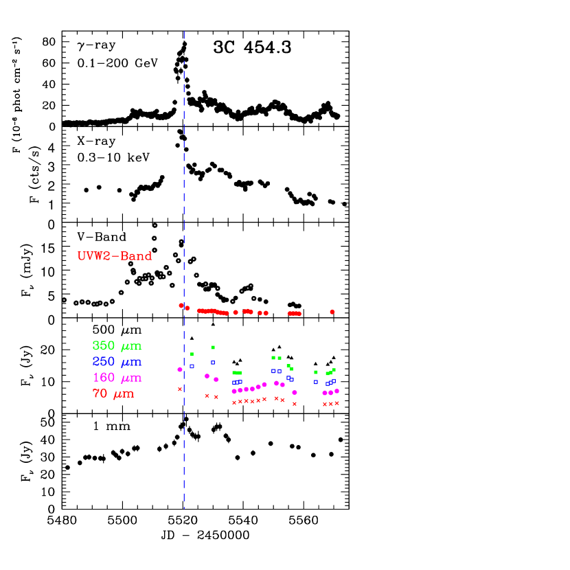
Figure 1: Light curves during November 2010-January 2011. From top: Fermi LAT $\gamma-$ray; Swift X-ray; V-band (filled circles are Swift V-band, open circles from SMARTS and Perkins Telescope); Swift UVW2 band (filled red circles); Herschel 500 (black triangles), 350 (filled green squares), 250 (open purple squares), 160 (filled magenta circles) and 70 (red crosses) $\mu$m bands; and SMA 1.3 mm band. The vertical dashed line is set at MJD 55520, the peak of the $\gamma-$ ray flare.

In some cases, we had several observations on the same day taken a few minutes apart in different scan directions or a few hours apart. We reduced each observation separately. The intra-day measurement differences were less than 2%, and in most cases less than 1%, well within the systematic errors; consequently, we averaged the data for each day. No color correction was applied (equivalent to assuming that $F_{\nu}\propto\nu^{-\alpha}$, with $\alpha=1$, or $\nu F_{\nu}=constant$ in SPIRE and PACS terminologies), since we did not know, a priori, the value of the spectral index over the Herschel bandpasses. We present the results in Table 1 and the light curves in Figure 1.

2.2 Submillimeter Array and IRTF Observations

The quasar 3C 454.3 is commonly used as an amplitude and phase calibrator at the SMA. Flux history measurements at wavelengths of 1.3 mm, 850 $\mu$m, and 450 $\mu$m of 3C 454.3 and several hundred other blazars in the Submillimeter Calibrator List, maintained by M. Gurwell, are provided online at http://sma1.sma.hawaii.edu. During the 2010 November to 2011 January period, we also observed the quasar as a science target. Data were reduced in the usual manner, as described in Gurwell et al. (2007). Data obtained at 225 GHz (1.3 mm) during the Herschel observing period are listed in Table 1.

The IRTF observations were performed with the MIRSI camera (Kassis et al., 2008) at central wavelengths of 4.9, 10.6, and 20.7 $\mu$m. We reduced the IRTF data with IDL using a script supplied by the IRTF staff, with calibration based on standard stars from the IRTF catalog.

2.3 Perkins Telescope and SMARTS Observations

We obtained optical photometric data at the 1.8 m Perkins Telescope of Lowell Observatory (Flagstaff, AZ) in BVR bands. We have employed differential photometry with comparison stars provided by Raiteri et al. (1998). The V-band optical data are supplemented by publicly available measurements by the SMARTS consortium (Charles Bailyn, PI), posted at their website http://www.astro.yale.edu/smarts/glast/. The V-band data are shown in Figure 1. Additional data and analysis will be given in Jorstad et al. (2012).

2.4 Swift Optical, Ultraviolet, and X-ray Observations

We analyzed all available data obtained by the Swift UVOT during the outburst that produced measurements of the flux density of 3C 454.3 in six filters, V (5402 Å), B (4329 Å), U (3501 Å), UW1 (2634 Å), UM2 (2231 Å), and UW2 (2030 Å). We employed the UVOT software task uvotsource to extract counts within a circular region of 5 arcsec radius for the source and 10 arcsec radius for the background, the latter centered 30 arcsec south-west of the source. We used the coefficients given in Table 1 of Raiteri et al. (2011) for correcting the derived magnitudes and flux densities for Galactic extinction. The de-reddened data are listed in Tables 2-4.

We used version 3.8 of the Swift Software (HEAsoft 6.11), with the version of CALDB released on 2011 June 9, to reduce the XRT data collected for 3C 454.3. During the outburst, from MJD 55457 to MJD 55578, the XRT obtained 67 measurements in Windowed Timing mode (WT) and 28 measurements in Photon Counting mode (PC). Observations in WT mode were performed during the brightest flux levels to avoid a pile-up effect on images, since from 2010 November 9 (MJD 55509) to December 24 (MJD 55554) the source count rate exceeded 1 count s^-1 at 0.3-10 keV and reached a maximum of 4.028$\pm$0.008 count s^-1 on November 19. We have downloaded Level 2 event files from the Swift Database Archive and reduced them in the manner described in the SWIFT XRT Data Reduction Guide, available on the Swift Data Analysis web page. The task xselect was used for extracting spectra of the source and background. In PC mode we used a circular aperture of 30 pixels for the source and an annulus with inner/outer radii of 110/160 pixels for the background. In WT mode, rectangular apertures equal in size to the circular and annular ones were applied along the brightest part of the window for the source and at the end of the window for the background. The tasks xrtmkarf and grppha were employed to produce the effective area file and to rebin the energy channels, respectively. Rebinned spectra were modelled within 0.3-10 keV in XSPEC v.12.7 with a single power-law and Galactic absorption corresponding to a hydrogen column density N_H = 6.50$\times$10²⁰ cm^-2 (Kalberla et al., 2005). We applied a Monte-Carlo method to estimate the goodness of fit of the model and derived 90% ($\sim$3-$\sigma$) confidence ranges of the fitted parameters (photon index and amplitude). The X-ray data are listed in Table 5.

2.5 Fermi LAT Data Analysis

We downloaded Pass 7 Fermi LAT data for the field surrounding 3C 454.3 from the data server of the Fermi Science Support Center (FSSC) at URL http://fermi.gsfc.nasa.gov/ssc. Reduction of the data utilized version v9r23p1 of the Fermi Science Tools software, associated background models, and a model of sources in the field (within $\sim 20^{\circ}$ of the position of 3C 454.3) generated from the 2FGL catalog by the script “make2FGLxml.py” by T. Johnson, available at the same website. We used the standard unbinned maximum likelihood analysis, integrating over short, 6-hour time bins and a photon energy range of 0.1-200 GeV. The $\gamma$-ray emission was detected at a test statistic value $>5$ (equivalent to about 2-$\sigma$; see Mattox et al., 1996) at all but one of the time intervals. The spectral model for 3C 454.3 was fixed to that given in the 2FGL catalog: a log-parabolic shape of the photon flux spectrum as a function of energy $E_{\gamma}$:

$$F(E_{\gamma})=F_{0}(E_{\gamma}/E_{b})^{-(\alpha+\beta\ln(E_{\gamma}/E_{b}))},$$ (1)

with $\alpha=2.23$, $\beta=0.118$, and $E_{b}=298$ MeV. We used a similar analysis for 24-hour binned data, except that we allowed the maximum likelihood algorithm to find the optimal values of $\alpha$, $\beta$, and $E_{b}$ rather than fixing them. The 24-hour-binned data are listed in Table 6. Because the errors in the log-parabolic model are correlated, their behavior is not simple, and we refer the reader to the technical discussion in the appendix of Tramacere et al. (2007). We have adopted the standard deviations of the $\alpha$, $\beta$ and break energies as uncertainties. Specifically, the errors are estimated at 6% in $\alpha$ and 15% for $\beta$ when the photon flux exceeds $10^{-5}$  $ph/s/cm^{2}$ and 35% below that level, and 30% in the break energy. (Running the maximum likelihood code on 24-hour binned data three times with different random number seeds resulted in changes of 1-2% in the values of alpha and beta.) There were too few photons when the data were binned in 24-hour bins to determine the break energy to better than about 30%. Our results are in general agreement with those of Abdo et al. (2011) who divided the flare episode into four unequal periods of several-to-many days each to obtain improved statistics using more photons. An additional contributor to the smaller error bars obtained by Abdo et al. follows from their use of a constant break energy while we allowed the break energy to vary.

2.6 VLBA Imaging

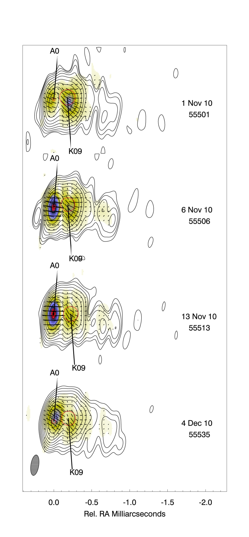
Figure 3: 43 GHz VLBA images of 3C 454.3 in November-December 2010, convolved with an elliptical restoring beam of FWHM dimensions $0.33\times 0.14$ mas oriented along position angle $-10^{\circ}$. Contours represent total intensity with levels in factors of 2 from 0.15% to 76.8% of the global peak brightness of 18.47 Jy beam^-1. Colors correspond to linearly polarized intensity with a global peak of 0.71 Jy beam^-1 (red). The short bars indicate the relative amplitude and direction of the polarization electric vector. The core (A0) and knot K09 are indicated with red circles delineating the FWHM size of the Gaussian model components. New knot K10 is blended with A0 on these images. The flux density of the core is 10.3, 14.1, 14.2, and 17.7 Jy (uncertainty $\approx 10\%$) from the first to the last image displayed. See Jorstad et al. (2012) for details.

We observed 3C 454.3 with the VLBA at 43 GHz in a manner similar to that described by Jorstad et al. (2010), where details of the data calibration and imaging can be found. Figure 3 presents four images from epochs within one month of the date of the maximum $\gamma$-ray flux during the outburst. The image features the bright, compact “core” A0 at the eastern end of the jet, as well as superluminal knot K09 that passed through the core during the late 2009 outburst. Observations with the VLBA in 2011 reveal that a new superluminal knot, K10 with an apparent speed of $\sim 9c$, was passing through the core during 2010 November (see Jorstad et al., 2012). The outburst in 3C 454.3 therefore provides us with an unprecedented opportunity to follow the evolution of a well-sampled SED as a superluminal knot traverses different regions of the jet.

3 Results

3.1 Light Curves and Spectral Indices

3.1.1 Herschel

The Herschel light curves are shown in Figure 1. The observations began on MJD 55519, yielding maximum flux densities of 13.8 and 7.61 Jy at 160 and 70 $\mu$m, respectively. The highest flux density was observed at 500 $\mu$m, on MJD 55530. The brightness decreased after this, interrupted by a brief rise on MJD 55550-55552 followed by further decline, with a slight upturn at the end of the observing window at MJD 55570-55571. Band-to-band spectral indices in the 1.3 mm - 70 $\mu$m range varied significantly, as measured on individual days. The overall variation was a factor of 1.8 at 500 $\mu$m, 1.7 at 350 $\mu$m, 1.7 at 250 $\mu$m, 2.1 at 160 $\mu$m, and 2.6 at 70 $\mu$m. The spectral indices, standard deviation and number of measurements (in parentheses) are: 1.3mm-500 $\mu$m: $0.64\pm 0.06(5)$, 500-350 $\mu$m: $0.59\pm 0.12(13)$, 350-250 $\mu$m: $0.81\pm 0.06,(13)$, 350-160 $\mu$m: $0.77\pm 0.10(3)$, 160-70 $\mu$m: $0.88\pm 0.07(14)$. Individual errors on the spectral indices are 2-4%.

3.1.2 SMA and IRTF

During the weeks leading up to the brightest days of the flare, the 1.3 mm flux density increased from a minimum of 3 Jy in April 2009 to a plateau of about 20-30 Jy, then began rising abruptly on MJD 55515. It peaked on MJD 55520 at $51.8\pm 4.3$ Jy, then declined to $41.8\pm 3.1$ Jy over the next few days. A brief flare to $47.5\pm 2.4$ Jy occurred on MJD 55529-55531, coincident with a high flux at 500 $\mu$m observed by Herschel. The mid-IR flux densities that we measured with the IRTF on 3 November 2010 were $0.293\pm 0.021$ Jy, $0.699\pm 0.037$ Jy, and $1.293\pm 0.195$ Jy at 4.9, 10.6, and 20.7 $\mu$m, respectively, so that the corresponding spectral indices were $\alpha_{4.9-10.6}=1.13\pm 0.11$ and $\alpha_{20.7-10.6}=0.92\pm 0.13$.

3.1.3 Swift UVOT and XRT

The Swift UVOT light curves in V, B, U, UVW1, UVM2, and UVW2 bands are presented in Figure 4; with additional V-band data from the Perkins Observatory and the SMARTS program. Inspection of this plot reveals that the main flare on MJD 55519-20 was preceded by a brightness plateau of abut two weeks, followed by two significant flares. The overall brightness variations were factors of 6.2, 5.8, 6.5, 3.9, 3.2, and 3.0 at V, B, U, UVW1, UVM2 and UVW2, respectively. Figure 4 also shows that the flare maximum occurred on MJD 55518-20, although the peaks at the various bands were not all simultaneous. This was followed by a gradual decline interspersed by two smaller flares.

The data in the six UVOT bands cannot be fit by a simple power-law because of features possibly caused by emission lines (e.g., a noticeable bump in the UVM2 spectrum caused by Ly$\alpha$, with smaller contributions by CIV in UVW1 and OVI+Ly$\beta$ in UVW2) and the Galactic interstellar dust absorption band at 2175 Å, as described by Raiteri et al. (2011) and references therein. These features are clearly visible in the overall millimeter-infrared-optical-ultraviolet SEDs in Figure 2. The spectral index using only V and UVW2 bands (ignoring the bumps and dips in between) can be readily calculated: it is much steeper at the flare peak than near the end of the Herschel observations — $1.70\pm 0.02$ on MJD 55519 and $1.00\pm 0.01$ on MJD 55558.

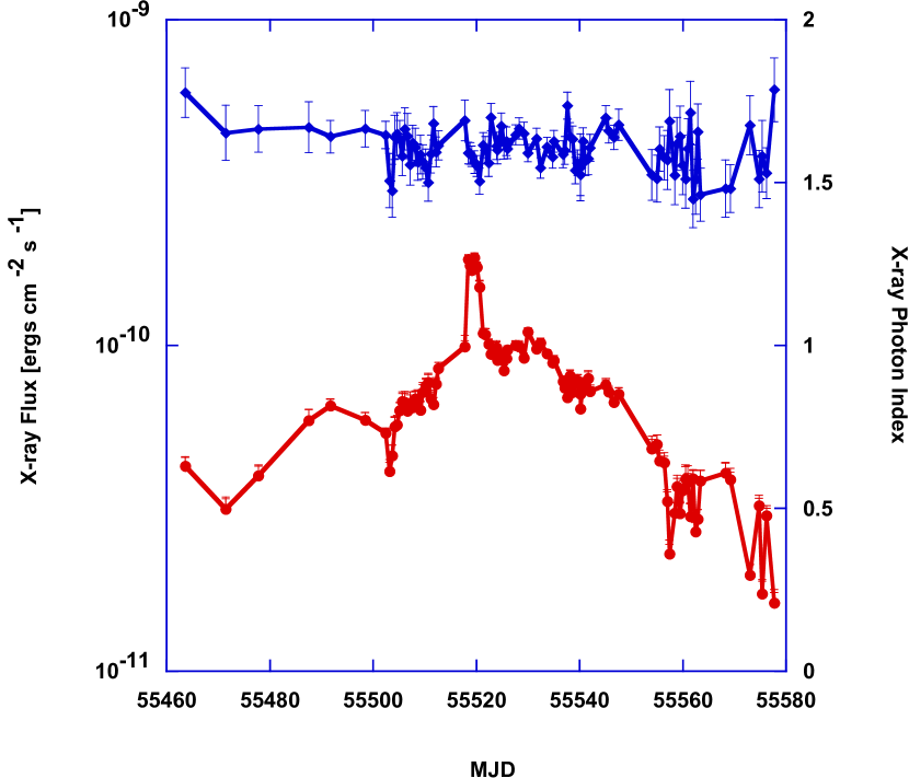
Figure 5: X-ray light curve (red circles) and photon index (blue diamonds) before, during and after the flare. The X-ray photon index varied between $\sim$ 1.5-1.7 and became slightly harder during the 2-3 days of the flare peak.

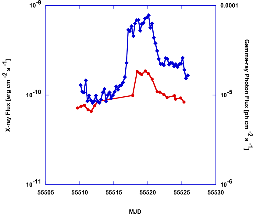
Figure 6: X-ray and $\gamma-$ray light curves centered on date of the main flare. X-ray flux (red circles) and 6-hour binned $\gamma-$ray photon flux (blue diamonds) show general agreement with differing details, especially during the peak of the flare.

The Swift X-ray light curve and photon spectral indices are presented in Figure 5. Figure 6 shows the X-ray and 6-hour-binned $\gamma$-ray light curves for fifteen days (MJD 55510-55525) encompassing the brightest days of the flare. The peak in the X-ray flare extended over five days between MJD 55517.7762 and MJD 55522.8419, with two nearly identical maxima of $1.84\times 10^{-10}\pm 5.9\times 10^{-12}$ erg cm^-2 s^-1 and $1.86\times 10^{-10}\pm 6.7\times 10^{-12}$ erg cm^-2 s^-1 on MJD 55517.7762 and MJD 55519.6305, respectively. During the brightest days of the flare on MJD 55519-20, the X-rays increased by a factor of 2.8, and the $\gamma$-rays by 8.9, over the low values on MJD 55511. The most substantial variation was observed between MJD 55517.7762 and 55518.4373, when the X-ray flux rose from $9.91\times 10^{-11}$ erg cm^-2 s^-1 to $1.84\times 10^{-10}$ erg cm^-2 s^-1, an increase of 86% in 16 hours. In contrast, Abdo et al. (2011) reported that the fastest $\gamma$-ray flux change was on MJD 55516.5, when the flux increased by a factor of 4 in 12 hours, for a doubling time of 6 hours. We have no Swift data between MJD 55512.6725 and 55517.7762, hence we cannot tell whether the X-ray and $\gamma$-ray flares rose exactly simultaneously on MJD 55516-55517.

During the Swift observations of the flare between MJD 55502 and 55577, the photon index increased from 1.45 to 1.79, with an average of $1.60\pm 0.06$. In the April 2008-March 2010 period, Raiteri et al. (2011) found that the photon index varied from 1.38 to 1.85, with an average value of 1.59, nearly the same as our value in November 2010-January 2011. During MJD 55502-55577, the X-ray flux varied from $1.62\times 10^{-11}\pm 1.4\times 10^{-12}$ ph cm^-2 s^-1 to $1.86\times 10^{-10}\pm 6.2\times 10^{-12}$ ph cm^-2 s^-1 (the latter on MJD 55519.6305), averaging $3.78\times 10^{-11}$ ph cm^-2 s^-1. There was no clear tendency for the photon index to flatten during the highest points of the flare. During the entire flare period, 3C 454.3 was much brighter than usual, and it did not return to very low, quiescent levels during the course of our observations.

3.1.4 Fermi LAT

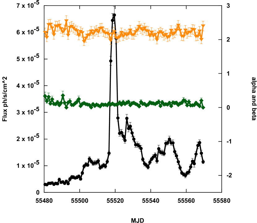
Figure 7: Fermi LAT $\gamma-$ray light curve made with 1-day bins. The photon flux is shown as black filled circles. The parameters of the log-parabolic fit, $\alpha$ and $\beta$, are shown as orange triangles and green diamonds, respectively. The errors on the photon flux are as shown in Table 6; we plot 6% errors on $\alpha$ and 35% errors on $\beta$. See text for discussion of correlated errors.

The $\gamma$-ray light curve based on 1-day binned data is displayed in Figure 7. The main flare peak around MJD 55519-20 was followed by a rapid decline with three smaller peaks occurring on MJDs 55526, 55550, and 55567. The minimum during the interval of the Herschel observations occurred on MJD 55558-9. Overall, the flux varied by a factor of 10.5 from MJD 55519.5 to 55559.5. As described by Abdo et al. (2011), $\gamma$-ray spectral variations were modest, although the spectrum flattened somewhat near the peak of the main flare. Within the log-parabolic spectral model that we have employed, this implies that the peak of the $\gamma$-ray SED shifted to somewhat higher energy as the flux peaked.

3.2 Correlations and Time Delays between Bands

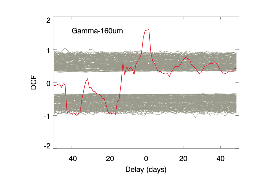
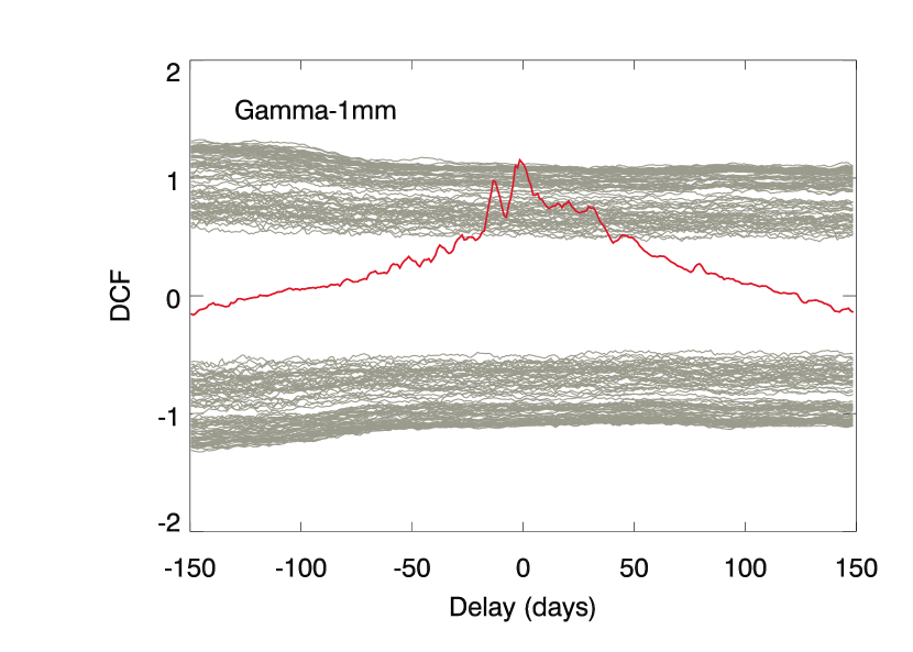
Figure 8: Discrete correlation function (red curve) for (Left) $\gamma-$ray and 160 $\mu$m data and (right) $\gamma-$ray and 1.3 mm data. Gray curves correspond to results of Monte Carlo simulations (see text). In both cases, the peak in the DCF has been fit with a Gaussian, from which we measure a delay of $-0.5$ to $+1.5$ days between $\gamma-$ray and 160 $\mu$m variations and $-1.5$ to +3.5 days between $\gamma-$ray and 1.3 mm variations.

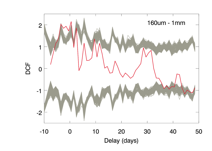
Figure 9: Discrete correlation function (DCF, red curve) for 160 $\mu$m and 1.3 mm data. Gray curves correspond to results of Monte Carlo simulations (see text). The DCF is not plotted if there are too few data points to calculate it at a given time delay, hence the red curve is discontinuous. The peak in the DCF has been fit with a Gaussian from which we measure a delay between $-3.5$ and $+0.5$ days.

We evaluate the time delays between bands by applying the discrete correlation function (DCF) methodology (Edelson & Krolik, 1988), as implemented in the aitlib library in IDL. In summary, the results of the DCF analysis indicate that variations at 0.1-200 GeV $\gamma$-ray energies, 160 $\mu$m, and 1.3 mm were simultaneous to within the accuracy of the method. For the correlation analysis, we supplement the 160 $\mu$m data with 250 $\mu$m data scaled by 0.724 (the average of the ratio of 250 $\mu$m to 160 $\mu$m flux densities on days when both bands were observed with different instruments on Herschel), resulting in 25 points in the light curve. The 1.3 mm SMA data over the time range from 2008 January 12 to 2011 October 27 are used with the original sampling (350 points). The Fermi LAT $\gamma$-ray light curve corresponds to one-day binned data from the beginning of science operations on 2008 August 5 to 2011 October 21 (1167 points). The resulting DCF curves are shown in Figures 8 and 9.

In order to determine the 3-$\sigma$ level of significance of a given correlation, we follow the methodology proposed by Chatterjee et al. (2008), Max-Moerbeck et al. (2010) and Agudo et al. (2011a). We simulate 5000 light curves for each of the three wavebands based on the mean, standard deviation, and slope $b$ of the power spectral density (PSD) of the observed flux variations. The PSD, which corresponds to the power in the variations as a function of timescale, is fit by a power law, $P(\tau)\propto\tau^{b}$, where $\tau$ is the time-scale of the variations. [According to Abdo et al. (2010), the PSDs of $\gamma$-ray light curves of quasars have average slopes of $\langle b\rangle=1.7$.] In the simulations, we vary the value of $b$ from 1.0 to 2.5 in increments of 0.1. The simulated light curves, binned in time in exactly the same way as the actual light curves, were cross-correlated to determine the probability of obtaining via random chance a particular value of the DCF at each relative time lag. This allows us to determine, for each pair of $b$ values, the level at which the measured DCF is significant with 99.7% confidence (3-$\sigma$), thus testing whether the observed correlation (or anti-correlation) is statistically significant. Curves representing these 99.7% confidence levels are drawn in gray in Figures 8 and 9.

Figures 8 and 9 show that (1) the correlation between the $\gamma$-ray and 160 $\mu$m light curves is significant for delays from -0.5 to +1.5 days (independent of the value of $b$), where a negative delay corresponds to $\gamma$-ray leading IR variations; (2) the correlation between the $\gamma$-ray and 1.3 mm light curves is significant and independent of the PSD slope for delays from -1.5 to +3.5 days, although there is a second DCF peak at -13.5$\pm$1 days that is significant for $b<$2.0 for both light curves; (3) the correlation between the 160 $\mu$m and 1.3 mm light curves is significant for delays from -3.5 to +0.5 days, where a negative delay corresponds to the IR variations leading.

The time delays at the peaks of the DCFs all include zero, but the offset from zero of the central values of the delays indicates that, on average, significant time lags occur. These are in the sense that the $\gamma$-ray variations lag those at 160 $\mu$m by $1\pm 0.5$ days, while the 1.3 mm variations lag those at 160 $\mu$m by $1.5\pm 2$ days. We therefore conclude that, to within the accuracy of our analysis, the variations are simultaneous at all three wavebands. Inspection of the profiles of the main flare confirm that the time lags were essentially zero for this event.

3.3 Relationship between Millimeter and Submillimeter Variations and Features on the VLBA Images

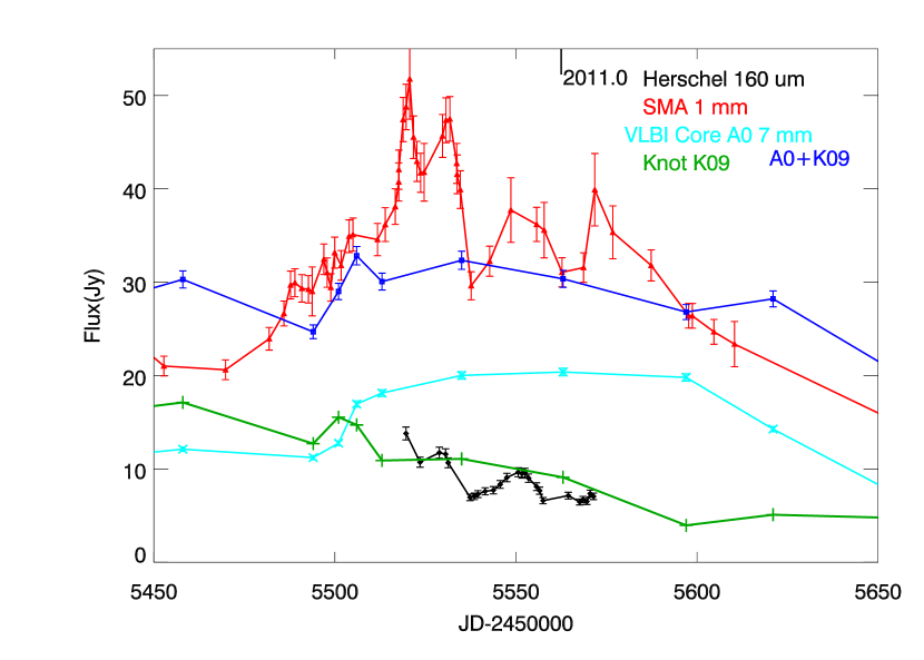
Figure 10: Light curves of total flux density observed at 160 $\mu$m (black diamonds; including interpolated fluxes based on 250 $\mu$m data), and 1.3 mm (red triangles), individual 43 GHz flux densities of the core A0 (purple Xs) and knot K09 (green crosses), and the sum of 43 GHz flux densities in the core A0 and Knot K09 (magneta squares and dotted line).

The sequence of VLBA images displayed in Figure 3 reveal two main emission features within 0.3 mas (2 pc projected distance) of the upstream end of the jet, A0 (the “core” plus new superluminal knot K10) and superluminal knot K09 that passed through the core in late 2009 (Jorstad et al., 2012). The images reveal a sharp increase in the brightness of the core during the first five weeks of the outburst. Figure 10 presents the 1.3 mm and 160 $\mu$m (including scaled 250 $\mu$m data) light curves along with that of A0 and K09 at 7 mm. If they are responsible for the 1.3 mm and far-IR emission, then A0 and/or K09 should vary synchronously with the SMA 1.3 mm and Herschel 160 $\mu$m fluxes. Indeed, the overall trend of the SMA flux matches that of A0 during the period MJD=55500 to 55580. The flux of K09, on the other hand, underwent a downward trend during the period shown, from about 16 Jy to 4 Jy. The nearly flat flux density spectrum between 225 GHz and 43 GHz (A0 + K09 only) is slightly inverted during the flare ($\alpha=-0.12$ to $-0.05$). Knot K09 must have possessed a steep spectral index, since the sum of the A0 and K09 fluxes exceeded the 1.3 mm flux before MJD 55500 when K09 was brighter than the core. The 7 mm A0 and 1.3 mm fluxes varied rapidly from MJD=55500 to 55515, on a time-scale much shorter than a month. Based on the overall behavior of the light curves, it is highly likely that the outburst at 1.3 mm is connected with the outburst in A0, although the data are ambiguous because the VLBA measurements happened to occur near or at local minima in the SMA light curve.

4 Spectral Energy Distributions

The combination of several satellite observatories and a number of ground-based telescopes has provided an extraordinarily rich dataset. The multi-waveband light curves provide both guidance and challenges for the development of theoretical models.

4.0.1 Overall Characteristics of 52 SEDs

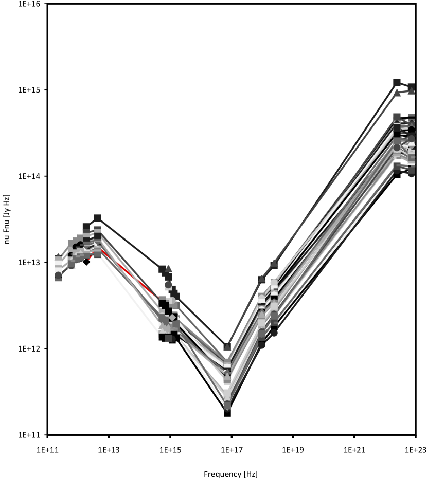
Figure 11: Spectral energy distributions obtained on 52 days during Nov 2010-Jan 2011 (MJD 55519-55571)and from the high state in 2005 (in red line visible from $\sim 10^{12}$ to $\sim 10^{15}$Hz ), the latter from Ogle et al. 2011. The gray-to-black shaded symbols and lines represent different dates. Note the similarity in overall appearance and that the 2005 high state SED blends in with the other SEDs.

We form 52 SEDs over the time interval of the near-daily observations, from 2010 November 19 to 2011 January 10 (see Tables 7 and 8). The SEDs are remarkably similar to each other, differentiated mainly by small day-to-day fluctuations (Figure 11). The peak amplitude of the synchrotron emission varied by a factor of $\sim 2$, while the peak amplitude of the inverse Compton emission varied by a factor of $\sim 10$. The millimeter to far-IR spectral indices (which vary only slightly) are very similar to the X-ray spectral indices (which are also essentially constant). The mid-IR SED, measured with the IRTF on 2010 November 3 near the start of the outburst, peaked at $\sim 15$ $\mu$m. We cannot determine whether the peak in the IR SED shifted upward in frequency during the flare as it did in 2005 (Ogle et al., 2011), since the maximum in the SED is not clearly defined by our Herschel far-IR observations. The peak in the $\gamma$-ray SED changed only modestly during the flare (see Fig. 11 and Abdo et al., 2011), although the low-energy cut-off to the $\gamma$-ray spectrum of 100 MeV reduces our ability to define the maximum when it is below $\sim 500$ MeV. Improvements in the $\it Fermi$ LAT data processing should allow extension of the measured spectra to lower energies in the future. This will provide further constraints on emission models.

Both during and after the peak of the flare, the difference between the submillimeter and optical spectral slopes exceeded the value of 0.5 which is expected from synchrotron and inverse Compton radiation losses. Specific details are as follows. Between the 1.3 mm and 160 $\mu$m bands, the spectral index $\alpha$ (where $S_{\nu}\propto\nu^{-\alpha}$) was $0.59\pm 0.02,0.72\pm 0.03,0.69\pm 0.03$ and $0.83\pm 0.03$ on MJDs 55519, 55531, 55537 and 55571, respectively. Between the 70 $\mu$m and Swift V band, the value of $\alpha$ was $1.27\pm 0.03,1.57\pm 0.04$, and $1.51\pm 0.04$ on MJDs 55519, 55531 and 55537, respectively (no Swift V band data were obtained on MJD 55571). The breaks in the synchrotron spectrum correspond to changes in slope of 0.68, 0.85, and 0.82.

The millimeter-infrared SEDs are shown in Figure 2. We note that at 350 $\mu$m, the SEDs showed an inflection point where the SED is higher than it would be with a linear interpolation between 500 $\mu$m and 250 $\mu$m. This small bump in the synchrotron peak during the declining phase of the outburst may be due to the superposition of two (or more) synchrotron-emitting components, or simply to inhomogeneities across a single emission feature. Given the steep spectrum of knot K09, its flux at 350 $\mu$m is far too low to cause the small bump at 350 $\mu$m. In 2005, the millimeter- infrared SED, observed with the SMA and Spitzer, contained a dip at 160 $\mu$m (Ogle et al., 2011), which was interpreted as the valley between two synchrotron peaks, one of which occurred between 850 $\mu$m and 160 $\mu$m where there was no observational data. We note that 3C 279 showed the same type of SED dip in Spitzer observations (Abdo et al., 2012). The dip is unlikely to be caused by an instrumental calibration problem, since it has been observed in two blazars by three different spacecraft (ISO, Spitzer, and Herschel) with independent instrument calibration strategies. Multiple or inhomogeneous emission regions therefore appear to be common features in the synchrotron SEDs of blazars.

The one-day binned Fermi LAT data were well-fit by a log parabolic model on most days, with one day on which the data were better fit by a power law. The amplitude of the $\gamma$-ray SED peak varied by a factor of $\sim$ 10 between the flare on MJD 55519 and the low, post-flare level of MJD 55558. The break energy was typically 300 MeV, with an increase to 345 MeV at the peak of the main flare.

The Herschel infrared observations began, coincidentally, on the day on which the flare peaked. The above correlation analysis of the far-IR and $\gamma$-ray light curves demonstrates that the variations were simultaneous, with any delays being less than about 1.5 days. While the very short time delays across frequencies indicate that a coherent emission zone is responsible for the outburst, the differences in the detailed flare profiles imply that there are irregularities in the physical conditions within that zone. These can take the form of gradients or spatial irregularities in the relativistic electron density and energy distribution or magnetic field strength and direction, for example.

The SMA 1.3 mm and 160-250 $\mu$m variations (Fig. 10) are also essentially simultaneous, with any delays less than 3.5 days. This indicates that the flaring synchrotron emission was optically thin at millimeter bands, and was probably dominated by a single variable component in late 2010. This contrasts with the conclusion of Ogle et al. (2011) that, several months after a major outburst in 2005, the emission arose from two components within a twisted jet. It also falsifies the model proposed by Vercellone et al. (2011) that places the site of the flare within a plasmoid of radius $3.6\times 10^{16}$ cm at a distance 0.05 pc from the center of the accretion disk. Besides locating the flare at a much smaller distance from the central engine than indicated by the VLBA observations, that model adopts physical parameters corresponding to an optical depth to synchrotron self-absorption of 5600 at 1.3 mm.

Examination of the light curves reveals that 3C 454.3 brightened significantly at both 1.3 mm and $\gamma$-ray energies weeks before the $\gamma$-ray brightness flared precipitously. This implies that the disturbance in the jet flow intensified gradually, starting well before the main flare began. The entire outburst therefore appears to be a prolonged event rather than an impulsive surge of energy, while the main flare does appear to be rather impulsive. This could be related to the complex structure (with three essentially stationary brightness peaks) of the core region inferred from analysis of VLBA images by Jorstad et al. (2010). The passage of a disturbance in the jet flow across each stationary feature in the jet would be expected to cause an outburst with complex temporal structure.

5 Theoretical Modeling of the SED

5.1 General Considerations

There are a number of features of the SED of 3C 454.3 during the outburst that any successful model should be able to reproduce. One is that the two SED peaks do not move sharply toward lower frequencies as the flux declines, as expected in expanding plasma blob or shock models (e.g., Marscher & Gear, 1985). The strong steepening of the spectra above the SED peaks from radiative energy losses after impulsive injection of relativistic electrons is also absent. Perhaps the most important aspect of the outburst is the general correspondence of the main flare at submillimeter to $\gamma$-ray wavelengths combined with significant dichotomy in flare substructure, as well as different amplitudes of the secondary flares, at the various wavebands. The similarity of the far-IR and X-ray spectral indices conforms with the expectations of the standard emission model for quasars in the blazar class, in which the radio to UV nonthermal emission is synchrotron radiation and the X-ray to $\gamma$-ray emission is inverse Compton scattering, with the same population of relativistic electrons responsible for both. We therefore interpret the data in terms of this scenario.

Previous interpretations of outbursts in $\gamma$-ray bright quasars concentrate on models in which the seed photons are from the accretion disk, BLR, or dust torus (e.g., Błażejowski et al., 2000; Sikora et al., 2009; Tavecchio et al., 2010; Vercellone et al., 2011). Such sources of seed photons from outside the jet can produce very high $\gamma$-ray fluxes in the observer’s frame owing to extra Doppler boosting of the seed photons in the plasma frame, as long as the emitting plasma is not well downstream of the source of seed photons. In these models, however, the seed photon field varies smoothly as the emitting plasma propagates down the jet. In contrast, the flares have jagged time profiles in 3C 454.3 and other blazars, and $\gamma$-ray and optical variations do not correspond well in detail (Bonning et al., 2009; Raiteri et al., 2011; Vercellone et al., 2011; Agudo et al., 2011b). In models in which the magnetic field is either uniform or completely chaotic, rapid fluctuations of the $\gamma$-ray flux would need to be caused by variations in the relativistic electron distribution, but these should affect the optical emission in the same way (see Marscher et al., 2010, for a discussion). A possible exception would be a model incorporating strong fluctuations in the velocity structure of the flow so that the Doppler factor varies across the emission region (Giannios, Uzdensky, & Begelman, 2009; Narayan & Piran, 2012).

The differences in the light curves can be caused by spatial and temporal variations in the direction of the magnetic field and/or acceleration of electrons. The former, which can be caused by turbulence in the jet flow, agrees with the polarization of the synchrotron emission. Time-variable degrees of polarization from a few to 30%, as observed at optical wavelengths in blazars — including 3C 454.3 in 2010 November (Jorstad et al., 2012) — can be reproduced by a model consisting of 10–100 cells of emission, each with a uniform magnetic field with random orientation relative to the other cells (Marscher & Jorstad, 2010).

The lack of strong evolution of the outburst toward lower frequencies favors emission by a stationary structure such as a standing shock rather than by a self-contained shock or plasmoid that expands as it moves down the jet. This leads us to adopt the scenario of Marscher & Jorstad (2010) in which turbulent plasma in the jet crosses a standing shock with a conical geometry (see also Cawthorne, 2006). Such a model is capable of producing different flare profiles at optical and $\gamma$-ray frequencies because the changing magnetic field direction strongly affects the synchrotron flux without much, if any, influence on the inverse Compton emission (Marscher, 2012). Further differences at the two wavebands can occur if there are strong velocity fluctuations in the flow that create spatial variations in the Doppler factor, or if the main source of seed photons is local to the jet, not spread out as would be the case for photons from the BLR or dusty torus.

5.2 Model Involving Turbulent Plasma Flowing across a Stationary Conical Shock Plus Mach Disk

In order to determine whether a model involving turbulent jet plasma flowing across a standing shock is capable of reproducing the observed nature of the outburst in 3C 454.3, we have calculated SEDs and light curves with the Turbulent Extreme Multi-Zone (TEMZ) numerical code developed by Marscher (2012). The geometry is sketched in Figure 12. A pressure mismatch at the boundary (with the interior of the jet being under-pressured) maintains a standing conical shock. A Mach disk, a strong shock oriented transverse to the jet axis with a radius much less than the cross-sectional jet radius, truncates the cone. Such a structure can occur when there is a high degree of azimuthal symmetry in the flow. The Mach disk slows the flow from a highly relativistic velocity to a speed no greater than $c/3$, where $c$ is the speed of light. This deceleration greatly compresses the magnetic field and density behind the shock front, so that the Mach disk radiates very efficiently. Since the flow crossing the conical shock is only modestly decelerated, it remains highly relativistic so that the plasma receives highly blueshifted emission from the Mach disk. The Mach disk therefore serves as a very intense source of seed photons that varies as the flow’s magnetic field and density of electrons change.

The TEMZ code divides the emission region beyond the shocks into many cylindrical cells, as illustrated in Figure 12. Each cell is assigned a uniform magnetic field whose direction is determined randomly. Relativistic electrons are injected into the cells at the shock front and subsequently lose energy from synchrotron and inverse Compton radiation as the plasma flows downstream. The jet opening angle is so small ($\lesssim 1^{\circ}$; Jorstad et al., 2005) that expansion cooling is negligible across the emission region. Although seed photons from the hot dust torus are included in the calculation, this source is negligible relative to the Mach disk synchrotron and first-order synchrotron self-Compton (SSC) radiation beyond several parsecs from the central engine. (Second-order SSC within the Mach disk is beyond the Klein-Nishina limit and therefore suppressed.) The Mach disk spectrum follows that of relativistic electrons in the “fast cooling” limit (Sari & Esin, 2001), but blueshifted by a factor that depends on the location of each cell. The energy density of the flow, constant throughout the jet cross-section at a given distance $z$ from the base, is allowed to vary randomly with time, and therefore with $z$, in a manner that reproduces the slope of the observed PSD of the $\gamma$-ray emission, $b\sim 1.7$ (Abdo et al., 2010). The energy density is split between the relativistic electrons and magnetic field, with the ratio of the two left as a free parameter. The calculations include synchrotron self-absorption within the cells and along the various photon paths.

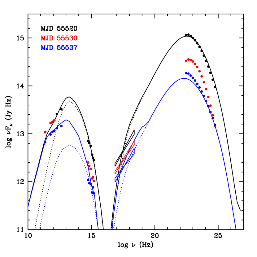
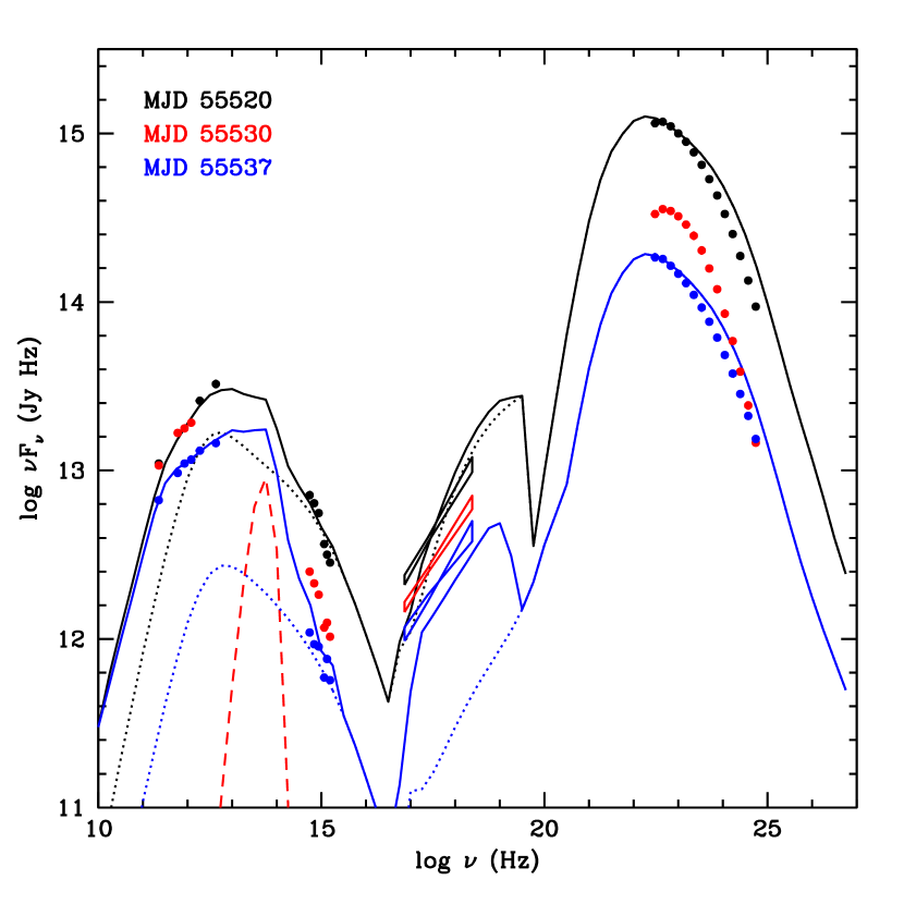
Figure 13: Spectral energy distributions from millimeter through $\gamma-$ray bands at three epochs. Dotted curves represent simulated SEDs generated by the TEMZ code at the peak of the light curve (black) and a later time (blue). The dashed red curve represents hot dust. Solid curves add to the TEMZ curves the more slowly varying emission observed prior to the outburst. Left model: seed photons are nonthermal radiation from Mach disk; Right model: seed photons are IR radiation from hot dust ($\gamma$-ray) and synchrotron radiation from plasma in cells (X-ray).

Since there is a strong random component in the TEMZ calculations, we cannot realistically reproduce the light curve of 3C 454.3 from the results of a reasonable number of accumulated time steps. [Marscher (2012) presents a sample light curve produced by the code.] Rather, we have searched enough parameter sets to determine that the simulated SED resembles that observed at the peak of the outburst, which was artificially induced by increasing the density of relativistic electrons by a factor of 10 over five time steps. We define this success as the ability to reproduce the spectral slopes within $\pm 0.1$ and the fluxes within a factor of two at all observed wavelengths. The left panel of Figure 13 presents one of the fits. The numerically induced flare is spread over a number of time steps owing to the propagation time down the conical shock and light-travel delays from the Mach disk to the various cells. The version of the code employed here incorporates 270 cells across the jet plus the Mach disk. Additional cells follow the emission in the flow beyond the conical shock until a rarefaction is reached, downstream of which expansion cooling is assumed to weaken the emission to a negligible level.

In the model, the steepening of the SED from IR to optical frequencies and toward higher $\gamma$-ray energies is a consequence of the electrons radiating in the optical and GeV bands having energies near the upper end of the electron distribution. These energies can only be maintained close to the injection site at the shock front, hence the volume filling factor is small relative to the emission by lower energy electrons at longer wavelengths. The dependence of the filling factor on frequency is such that the SED can be fit fairly well as a power law over a decade or more in frequency. Our fits to the SED of 3C 454.3 shown in Figure 13 are only representative, and surely not unique, given that we have explored only a relatively narrow range of free parameters. Fits to the SEDs on MJD 55520 and 55537 are quite good; the run of TEMZ that produced these SEDs missed the intermediate-state SED of MJD 55530 owing to the finite time steps inherent to the code, combined with the rapid drop of flux during the declining stage of the flare. We set the bulk Lorentz factor of the unshocked flow at 30 and the angle between the jet axis and the line of sight at $0.3^{\circ}$, as derived from the VLBA observations (Jorstad et al., 2012). In our frame, a given cell of plasma propagates down the jet at a rate of 0.8 pc day^-1 until it crosses the shock and decelerates. This causes very rapid time-scales of variability as turbulent cells enter the shock. Besides the injected electron energy, the free parameters (and their adopted values) include the angle of the conical shock to the jet axis ($4^{\circ}$, which yields a bulk Lorentz factor of the shocked plasma of 13.9 and a mean Doppler factor of 24), ratio of electron to magnetic energy density (12 in quiescence), time-averaged pre-shocked magnetic field strength (0.016 G), cell cross-sectional radius (0.008 pc), and cross-sectional radius of the Mach disk (0.016 pc). The hardening of the $\gamma$-ray spectrum at energies $>10$ GeV after the maximum flux of the flare found by Abdo et al. (2011) occurs also in the SED produced by the TEMZ code: Figure 13 shows a flatter $\gamma$-ray spectral slope above the peak in the SED during the decaying portion of the flare. This is expected because lower flux levels reduce the radiative energy loss rate of the highest-energy electrons. As the flux declines, more of these electrons can therefore maintain their energies long enough to make $>10$ GeV photons via inverse Compton scattering.

Although the fit to the observed SED is not unique, other parameter sets providing similar fits do not vary greatly from these values. The only significant discrepancy with the data is in the X-ray spectral index $\alpha_{\rm x}$. This is 0.5 in the model, while the observations give a value of $\sim 0.7$. The spectral index from the model calculation reflects the slope of the electron energy distribution, which is $-2.0$ at energies below the minimum injected energy owing to the dependence of the radiative energy loss rate on the square of the energy. The fit to the slopes in the other observed frequency ranges is quite good, on the other hand.

5.3 Model Involving Turbulent Plasma Flowing across a Stationary Conical Shock Irradiated by IR Emission from Hot Dust

The failure of the TEMZ model with a Mach disk to fit the X-ray data might be the result of limiting the geometry to uniformity across each cross-section of the pre-shocked flow or some other simplification. It could also indicate that another source of seed photons dominates the inverse Compton scattering by electrons in the jet of 3C 454.3. In order to investigate this possibility, we have also performed a calculation with a different source of seed photons for inverse Compton scattering: thermal IR emission by dust. We adopt the standard geometry of a torus, allowing for a patchy structure. Since dust emission in a blazar has been observed directly with a well-characterized SED only in 4C 21.35 (Malmrose et al., 2011), we use the IR SED of this blazar as the standard. The emission is dominated by a blackbody of temperature 1200 K with a luminosity of $8\times 10^{45}$ erg s^-1, which is 22% of the accretion disk luminosity. We note that the disk luminosity of 3C 454.3 is about 50% that of 4C 21.35 (Vercellone et al., 2011). If the dust of the latter blazar is confined to a uniform torus, the inner radius is 1.1 pc and the outer radius 1.9 pc (Malmrose et al., 2011). The torus might actually be larger if it is patchy, but at the expense of a lower filling factor of its emission as viewed in the frame of the jet plasma.

We have included thermal emission from such a dust torus in the TEMZ model after removing the Mach disk, which is appropriate if substantial azimuthal asymmetries exist in the pressure of the jet or surrounding confining medium. We used the dust luminosity that is the maximum allowed by the data. The right panel of Figure 13 displays SEDs at two times produced in a simulation that provides a rather good fit to the synchrotron and $\gamma$-ray SEDs. Inverse Compton scattering of the dust-emitted IR photons greatly under-produces the X-ray emission. SSC emission (calculated only crudely in the current version of the TEMZ code, which includes only synchrotron seed photons from a cell and its nearest neighbors) produces an X-ray flux similar to the observed value at the peak of the main flare. The parameters used in the model that differ from those in the Mach disk scenario are: pre-shocked mean magnetic field of 0.01 G, ratio of electron to magnetic energy density of 100, cell cross-sectional radius of 0.005 pc, minimum and maximum energy of electrons of $10^{3}$ and $2\times 10^{4}$ times $mc^{2}$, and shock angle of $3.0^{\circ}$ to the jet axis. In order to create a sufficient density of seed photons, the dust torus is allowed to be rather large, with an outer radius of 7 pc and inner radius of 3 pc. We set the areal covering factor at 0.1 such that the IR luminosity exceeds that expected based on the disk luminosity by a factor of 3, which allows us to place the upstream end of the conical shock at 1 pc from the central engine, while the downstream end is at 2.8 pc. If we were to place the emission farther downstream, the hot dust would need to be spread over an even larger volume to produce enough seed photons to explain the apparent luminosity of the outburst.

Because the dust torus provides a steady source of seed photons that declines with distance down the jet, the outward motion of the disturbance can cause the declining portion of a flare. However, any more rapid fluctuations need to arise from either a change in the electron density or energy distribution — in which case the same fluctuation should appear in both the optical and $\gamma$-ray light curves, since the emission at both regions arises from the same electrons — or variations in the Doppler factor from cell to cell. The TEMZ code does not yet include the latter.

5.4 Other Possible Sources of Seed Photons

It is possible that seed photons for inverse Compton scattering could arise from other sources in the nucleus of the blazar. One of these is nonthermal radiation from a somewhat slower sheath of the jet that may surround the extremely relativistic “spine” (see Marscher et al., 2010, and references therein). This emission might be more local to the primary $\gamma$-ray emission region, perhaps allowing variability on the observed intra-day time-scales (Abdo et al., 2011; Vercellone et al., 2011). Although the TEMZ code does not yet include seed photons from the sheath, the resulting emission pattern should be fairly similar to that of the model that includes seed photons from a Mach disk. The main difference is that emission from the sheath would not be as concentrated, which would broaden the flare profiles. In addition, the disturbance causing the flare would propagate at a slower speed in the sheath, so that the amplification of the flare via an increase in both the number of radiating electrons and density of seed photons in the Mach disk model would not occur.

León-Tavares et al. (2011) have proposed that emission-line clouds situated near the jet on parsec scales could provide local sources of seed photons. In this case, the emission-line luminosity would be expected to vary along with the nonthermal UV continuum, contrary to observations of both 3C 454.3 during the outburst studied here (Jorstad et al., 2012) and the $\gamma$-ray bright quasar 4C 21.35 during a multi-waveband outburst in 2010 (Smith, Schmidt, & Jannuzi, 2011).

6 Conclusions

The variations of flux at millimeter, far-IR, and $\gamma$-ray bands during the outburst of 3C 454.3 from 2010 November to 2011 January were strongly correlated, with the $\gamma$-ray variations lagging those at 1.3 mm and 160 $\mu$m by $1.0\pm 0.5$ days. Despite the strong correlations, the substructure of the outburst reveals significant differences at various wavebands. This suggests that physical substructure is present in the jet, which we interpret as evidence for turbulent processes.

The nearly simultaneous peak of the main flare at 1.3 mm and at $\gamma$-ray energies implies that the flaring component of the multiwavelength emission was optically thin and dominated the emission at frequencies higher than 43 GHz. At 1.3 mm, the core region and knot K09 (ejected in late 2009) were the main emitters. Analysis of the light curve of the two components leads to the conclusion that the core region was responsible for the 1.3 mm outburst, while the flux of K09 declined during the event. The lack of a significant time delay between the flare at 1.3 mm and $\gamma$-ray energies requires that the flare takes place in a region that is transparent at 1.3 mm. In support of this, the core region brightened by 70% at 7 mm during the early stages of the outburst bracketing the main flare. The data therefore favor a location of the outburst within the parsec-scale core rather than within the BLR. This conflicts with the model proposed by Vercellone et al. (2011), who place the flare in a region $3.6\times 10^{16}$ cm in radius only 0.05 pc from the central engine. In addition, later VLBA observations have identified a bright superluminal knot that was blended with the core during the outburst. The disturbance creating the flare therefore appears to have created the new knot.

Our Herschel far-IR observations clearly define the low-frequency side of the maximum in the synchrotron SED, from which we infer that the SED peaked at a wavelength shorter than 70 $\mu$m. Two weeks before the flare, IRTF observations located the peak at 11 $\mu$m. The SED of the main flare did not shift toward lower frequencies as rapidly as expected in shock or expanding plasmoid models. This leads us to interpret the outburst in terms of a standing shock in the jet, across which turbulent plasma flows. A major increase in the energy density of the plasma causes an outburst as it crosses the shock, which has a conical structure. If the conical shock terminates in a transversely oriented Mach disk, a strong shock that decelerates and compresses the flow greatly, emission from the Mach disk can provide the main source of seed photons for inverse Compton scattering to generate the X-ray and $\gamma$-ray emission. The TEMZ code produces model SEDs, following this scenario, that match the millimeter to optical and $\gamma$-ray spectra quite well although the observed X-ray spectrum is somewhat steeper than in the model calculations. Alternatively, if asymmetries in the jet flow prevent the formation of a Mach disk, thermal IR emission from hot dust can provide the requisite seed photons. However, the dust would need to have a luminosity $\sim 1\times 10^{46}$ erg s^-1 — half that of the accretion disk — and would need to be very patchy. In the TEMZ model, the volume filling factor of the emission is inversely related to the frequency of observation. Because of this, the average degree of linear polarization, as well as the level of variability of both the flux and polarization, should increase with frequency in a manner that is quantitatively related to the amount of steepening of the spectral slope toward high frequencies (Marscher & Jorstad, 2010). Another prediction of the model is that details of the flare profiles should change randomly from one flare to another.

Our observations of 3C 454.3 therefore present significant challenges to all theoretical models that have been proposed thus far. Since the polarization properties of blazars require irregularities in the magnetic field that are most easily understood as the effects of turbulence, scenarios similar to the TEMZ model appear to be necessary to reproduce the observed multi-waveband behavior of blazars. Whether this class of models can succeed in doing so requires further development of such models as well as more comprehensive observations of distinct outbursts in blazars.

Figure 2: Spectral energy distributions from millimeter through ultraviolet bands. The symbols and colors represent different MJDs.

Figure 4: Swift UVOT lightcurves before, during and after flare. Filter bands include V (red circles), B (orange inverted triangles), U (green diamonds), UVW1 (blue squares), UVM2 (pink-red crosses), and UVW2 (purple triangles). Dereddening has been applied as described in Raiteri et al. 2011.

Figure 12: Sketch of geometry adopted in the TEMZ model. Top: View down the jet, whose cross-section is divided into many cylindrical cells. Actual calculations displayed in Fig. 13 use 271 cells across the jet. Bottom: Side-on view. Cylindrical cells appear as rectangles. The conical shock compresses the flow & accelerates electrons. The Mach disk, if present, is at the axis, oriented transverse to the flow.

Table 1: SMA and Herschel Data

Date	MJD	1.3 mm	1.3 mm	500 µm	350 µm	250 µm	160 µm	70 µm
		Flux	Flux	Flux	Flux	Flux	Flux	Flux
		Density	Density Error	Density	Density	Density	Density	Density
		[Jy]	[Jy]	[Jy]	[Jy]	[Jy]	[Jy]	[Jy]
19-Nov-2010	55519	48.8	2.4	$\cdots$	$\cdots$	$\cdots$	13.8	7.61
20-Nov-2010	55520	51.8	4.3	$\cdots$	$\cdots$	$\cdots$	$\cdots$	$\cdots$
21-Nov-2010	55521	45.5	2.3	$\cdots$	$\cdots$	$\cdots$	$\cdots$	$\cdots$
22-Nov-2010	55522	42.9	2.1	$\cdots$	$\cdots$	$\cdots$	$\cdots$	$\cdots$
23-Nov-2010	55523	41.7	2.1	23.48	18.63	14.81	$\cdots$	$\cdots$
24-Nov-2010	55524	41.8	3.1	$\cdots$	$\cdots$	$\cdots$	$\cdots$	$\cdots$
25-Nov-2010	55525	$\cdots$	$\cdots$	$\cdots$	$\cdots$	$\cdots$	$\cdots$	$\cdots$
26-Nov-2010	55526	$\cdots$	$\cdots$	$\cdots$	$\cdots$	$\cdots$	$\cdots$	$\cdots$
27-Nov-2010	55527	$\cdots$	$\cdots$	$\cdots$	$\cdots$	$\cdots$	$\cdots$	$\cdots$
28-Nov-2010	55528	$\cdots$	$\cdots$	$\cdots$	$\cdots$	$\cdots$	11.74	5.53
29-Nov-2010	55529	45.7	2.3	$\cdots$	$\cdots$	$\cdots$	$\cdots$	$\cdots$
30-Nov-2010	55530	47.4	2.4	27.91	20.75	15.99	$\cdots$	$\cdots$
1-Dec-2010	55531	47.5	2.4	$\cdots$	$\cdots$	$\cdots$	10.66	5.19
2-Dec-2010	55532	$\cdots$	$\cdots$	$\cdots$	$\cdots$	$\cdots$	$\cdots$	$\cdots$
3-Dec-2010	55533	42.7	2.1	$\cdots$	$\cdots$	$\cdots$	$\cdots$	$\cdots$
4-Dec-2010	55534	39.9	2.0	$\cdots$	$\cdots$	$\cdots$	$\cdots$	$\cdots$
5-Dec-2010	55535	$\cdots$	$\cdots$	$\cdots$	$\cdots$	$\cdots$	$\cdots$	$\cdots$
6-Dec-2010	55536	$\cdots$	$\cdots$	$\cdots$	$\cdots$	$\cdots$	$\cdots$	$\cdots$
7-Dec-2010	55537	29.6	1.5	16.09	12.79	9.66	6.95	3.38
8-Dec-2010	55538	$\cdots$	$\cdots$	15.49	12.75	9.77	$\cdots$	$\cdots$
9-Dec-2010	55539	$\cdots$	$\cdots$	16.59	12.75	9.96	7.3	3.74
10-Dec-2010	55540	$\cdots$	$\cdots$	$\cdots$	$\cdots$	$\cdots$	$\cdots$	$\cdots$
11-Dec-2010	55541	$\cdots$	$\cdots$	$\cdots$	$\cdots$	$\cdots$	7.6	3.93
12-Dec-2010	55542	32.3	1.6	$\cdots$	$\cdots$	$\cdots$	$\cdots$	$\cdots$
13-Dec-2010	55543	$\cdots$	$\cdots$	$\cdots$	$\cdots$	$\cdots$	7.72	3.77
14-Dec-2010	55544	$\cdots$	$\cdots$	$\cdots$	$\cdots$	$\cdots$	$\cdots$	$\cdots$
15-Dec-2010	55545	$\cdots$	$\cdots$	$\cdots$	$\cdots$	$\cdots$	8.34	4.08
16-Dec-2010	55546	$\cdots$	$\cdots$	$\cdots$	$\cdots$	$\cdots$	$\cdots$	$\cdots$
17-Dec-2010	55547	$\cdots$	$\cdots$	$\cdots$	$\cdots$	$\cdots$	9.08	4.47
18-Dec-2010	55548	37.7	3.5	$\cdots$	$\cdots$	$\cdots$	$\cdots$	$\cdots$
19-Dec-2010	55549	$\cdots$	$\cdots$	$\cdots$	$\cdots$	$\cdots$	$\cdots$	$\cdots$
20-Dec-2010	55550	$\cdots$	$\cdots$	19.95	17.52	13.31	$\cdots$	$\cdots$
21-Dec-2010	55551	$\cdots$	$\cdots$	$\cdots$	$\cdots$	$\cdots$	9.5	4.71
22-Dec-2010	55552	$\cdots$	$\cdots$	20.78	17.35	13.24	$\cdots$	$\cdots$
23-Dec-2010	55553	$\cdots$	$\cdots$	$\cdots$	$\cdots$	$\cdots$	9.01	4.22
24-Dec-2010	55554	$\cdots$	$\cdots$	$\cdots$	$\cdots$	$\cdots$	$\cdots$	$\cdots$
25-Dec-2010	55555	36.2	1.8	17.68	15.01	11.19	$\cdots$	$\cdots$
26-Dec-2010	55556	$\cdots$	$\cdots$	17.36	14.02	10.60	$\cdots$	$\cdots$
27-Dec-2010	55557	35.6	3.0	$\cdots$	$\cdots$	$\cdots$	6.6	2.98
28-Dec-2010	55558	$\cdots$	$\cdots$	$\cdots$	$\cdots$	$\cdots$	$\cdots$	$\cdots$
29-Dec-2010	55559	$\cdots$	$\cdots$	$\cdots$	$\cdots$	$\cdots$	$\cdots$	$\cdots$
30-Dec-2010	55560	$\cdots$	$\cdots$	$\cdots$	$\cdots$	$\cdots$	$\cdots$	$\cdots$
31-Dec-2010	55561	$\cdots$	$\cdots$	$\cdots$	$\cdots$	$\cdots$	$\cdots$	$\cdots$
1-Jan-2011	55562	31.1	1.6	$\cdots$	$\cdots$	$\cdots$	$\cdots$	$\cdots$
2-Jan-2011	55563	$\cdots$	$\cdots$	$\cdots$	$\cdots$	$\cdots$	$\cdots$	$\cdots$
3-Jan-2011	55564	$\cdots$	$\cdots$	15.51	12.92	9.87	$\cdots$	$\cdots$
4-Jan-2011	55565	$\cdots$	$\cdots$	$\cdots$	$\cdots$	$\cdots$	$\cdots$	$\cdots$
5-Jan-2011	55566	$\cdots$	$\cdots$	$\cdots$	$\cdots$	$\cdots$	$\cdots$	$\cdots$
6-Jan-2011	55567	$\cdots$	$\cdots$	$\cdots$	$\cdots$	$\cdots$	6.46	2.89
7-Jan-2011	55568	31.6	1.6	15.32	12.55	9.28	$\cdots$	$\cdots$
8-Jan-2011	55569	$\cdots$	$\cdots$	16.09	12.83	9.68	6.52	2.98
9-Jan-2011	55570	$\cdots$	$\cdots$	17.48	13.68	10.16	$\cdots$	$\cdots$
10-Jan-2011	55571	39.9	3.9	$\cdots$	$\cdots$	$\cdots$	7.06	3.2

Table 2: Swift UVOT V and B Band Photometry

MJD	V band	V band	MJD	B band	B band
	Flux	Flux		Flux	Flux
	Density	Density Error		Density	Density Error
	[mJy]	[mJy]		[mJy]	[mJy]
55471.4764	3.67	0.13	55471.4739	3.01	0.07
55477.8188	3.13	0.08	55477.8133	2.34	0.04
55491.7490	2.61	0.07	55487.5339	2.56	0.04
55498.5102	4.00	0.08	55491.7421	2.13	0.04
55502.4454	10.49	0.12	55498.5036	2.98	0.04
55504.1962	6.59	0.12	55502.4385	7.30	0.06
55504.6523	7.14	0.13	55504.1914	4.97	0.06
55505.1875	7.22	0.12	55504.6474	5.17	0.06
55506.1915	7.48	0.14	55505.1824	5.37	0.06
55507.1990	7.47	0.13	55506.1872	5.48	0.06
55508.2014	8.99	0.14	55507.1944	5.49	0.06
55509.2012	7.05	0.12	55508.1962	6.52	0.06
55510.2079	13.91	0.17	55509.1960	5.35	0.06
55511.2149	7.97	0.13	55510.2030	11.14	0.08
55512.2134	8.65	0.12	55511.2097	6.09	0.06
55519.6408	15.21	0.15	55512.2070	6.29	0.06
55525.3410	7.02	0.11	55519.6348	11.13	0.07
55525.8762	6.85	0.10	55525.3344	5.32	0.05
55526.0682	6.84	0.11	55525.8693	5.13	0.05
55527.6162	5.98	0.11	55526.0622	5.26	0.05
55528.2786	6.15	0.10	55527.6104	4.57	0.05
55529.2069	6.72	0.11	55528.2711	4.72	0.05
55530.0124	6.76	0.12	55529.2011	5.06	0.06
55531.6892	4.89	0.10	55530.0069	4.89	0.06
55532.4234	4.34	0.11	55531.6837	3.59	0.05
55533.7044	3.61	0.09	55532.4194	2.82	0.05
55534.7776	3.76	0.13	55533.6984	2.68	0.04
55537.1743	4.17	0.08	55534.7748	2.46	0.06
55537.6518	5.55	0.09	55537.1660	3.11	0.04
55540.1942	6.09	0.12	55537.6437	4.09	0.04
55542.0613	6.13	0.13	55540.1897	4.66	0.06
55545.0820	3.86	0.10	55542.0570	4.63	0.06
55547.6229	3.39	0.08	55545.0768	2.76	0.05
55555.5093	2.71	0.07	55547.6155	2.55	0.04
55556.4455	2.88	0.07	55555.5030	1.98	0.04
55557.4470	2.45	0.08	55556.4386	2.16	0.04
55558.9241	2.49	0.08	55557.4412	1.98	0.04
$\cdots$	$\cdots$	$\cdots$	55558.9184	1.94	0.04

Table 3: Swift UVOT U and UVW1 Band Photometry

MJD	U band	U band	MJD	UVW1 band	UVW1 band
	Flux	Flux		Flux	Flux
	Density	Density Error		Density	Density Error
	[mJy]	[mJy]		[mJy]	[mJy]
55471.4734	2.45	0.05	55471.4726	1.63	0.03
55477.8122	1.94	0.03	55477.8106	1.33	0.02
55487.5328	1.82	0.03	55487.5312	1.31	0.02
55491.7407	1.79	0.03	55491.7386	1.31	0.02
55498.5022	2.29	0.03	55498.5002	1.49	0.02
55502.4371	5.07	0.04	55502.4350	2.75	0.02
55504.1904	3.43	0.04	55503.1719	2.40	0.02
55504.6464	3.58	0.04	55503.7221	2.09	0.01
55505.1813	3.75	0.04	55504.1889	2.08	0.02
55506.1863	4.09	0.04	55504.6449	2.16	0.02
55507.1935	4.15	0.04	55505.1797	2.25	0.02
55508.1952	4.71	0.04	55506.1850	2.28	0.03
55508.6654	4.54	0.01	55507.1921	2.40	0.03
55509.1950	3.90	0.04	55507.6630	2.77	0.01
55510.2020	8.42	0.05	55508.1936	2.87	0.03
55511.2086	4.36	0.04	55509.1934	2.48	0.03
55512.2057	4.50	0.04	55510.2005	4.98	0.04
55512.6794	4.45	0.01	55511.2071	2.59	0.03
55519.6336	7.83	0.05	55511.6874	2.81	0.01
55520.1052	9.81	0.01	55512.2038	2.68	0.02
55520.6427	9.95	0.02	55519.1017	4.21	0.01
55524.0650	4.10	0.05	55519.6318	4.30	0.03
55524.8648	4.06	0.01	55523.3842	3.14	0.01
55525.3331	3.70	0.03	55523.9205	2.50	0.01
55525.8679	3.75	0.03	55525.3311	2.24	0.02
55526.0610	3.62	0.04	55525.8658	2.33	0.02
55527.6093	3.32	0.04	55526.0591	2.06	0.02
55528.2696	3.27	0.03	55527.6075	2.03	0.02
55529.2000	3.62	0.04	55528.2673	2.11	0.02
55530.0058	3.50	0.04	55529.1982	2.14	0.02
55531.6826	2.55	0.03	55530.0042	2.05	0.02
55532.4186	2.18	0.04	55531.6809	1.67	0.02
55533.6972	2.05	0.03	55532.4174	1.50	0.02
55534.7742	1.96	0.04	55533.6953	1.39	0.02
55536.7833	2.10	0.02	55534.7734	1.37	0.03
55537.1643	2.43	0.03	55535.0231	1.35	0.01
55537.6421	2.85	0.03	55537.1618	1.55	0.02
55540.1798	3.03	0.01	55537.6396	1.90	0.02
55540.1887	3.30	0.04	55539.1864	1.78	0.01
55540.6610	3.25	0.01	55539.6572	1.82	0.01
55542.0561	3.15	0.04	55540.1873	1.86	0.02
55545.0758	2.11	0.03	55542.0548	1.96	0.03
55547.6140	2.04	0.03	55545.0742	1.39	0.02
55555.5017	1.75	0.03	55547.6117	1.36	0.02
55556.4372	1.65	0.03	55555.0380	1.18	0.01
55556.9791	1.65	0.01	55555.4998	1.15	0.02
55557.4401	1.55	0.03	55556.4351	1.19	0.02
55558.9172	1.58	0.03	55557.4383	1.18	0.02
55560.5223	1.53	0.01	55558.9155	1.10	0.02
55560.9900	1.53	0.01	55559.5190	1.12	0.01
55564.4089	2.15	0.03	55559.9851	1.10	0.01
55564.9439	2.17	0.04	55563.4658	1.99	0.04
55568.2842	1.88	0.02	55563.9403	1.97	0.12
55576.2530	2.21	0.02	55575.3869	2.02	0.04

Table 4: Swift UVOT UVM2 and UVW2 Band Photometry

MJD	UVM2 band	UVM2 band	MJD	UVW2 band	UVW2 band
	Flux	Flux		Flux	Flux
	Density	Density Error		Density	Density Error
	[mJy]	[mJy]		[mJy]	[mJy]
55471.4773	1.45	0.03	55471.4752	1.22	0.02
55477.8208	1.30	0.02	55477.8160	1.02	0.01
55491.7516	1.21	0.02	55487.5364	0.96	0.01
55498.5128	1.30	0.02	55491.7455	0.95	0.01
55502.4481	2.28	0.02	55498.5069	0.96	0.01
55504.1981	1.70	0.02	55502.4419	1.71	0.01
55504.6542	1.90	0.02	55504.1938	1.36	0.01
55505.1895	1.87	0.02	55504.6499	1.44	0.01
55506.1932	2.08	0.02	55505.1849	1.54	0.01
55506.6576	2.03	0.01	55505.6543	1.41	0.01
55507.2008	2.17	0.02	55506.1893	1.57	0.01
55508.2034	2.49	0.02	55507.1967	1.58	0.01
55509.2033	2.11	0.02	55508.1988	1.97	0.01
55510.2098	4.17	0.03	55509.1986	1.57	0.01
55510.6714	3.12	0.01	55509.6689	1.86	0.01
55511.2168	2.40	0.02	55510.2055	3.38	0.02
55512.2157	2.41	0.02	55511.2123	1.75	0.01
55518.4441	3.21	0.01	55512.2102	1.85	0.01
55518.8333	3.57	0.01	55517.7806	2.25	0.01
55519.6430	3.27	0.03	55519.6378	2.60	0.02
55522.3807	2.41	0.01	55521.3771	2.05	0.01
55522.8491	2.76	0.01	55521.7795	2.13	0.01
55525.3435	1.83	0.02	55525.3377	1.48	0.01
55525.8788	1.87	0.02	55525.8728	1.47	0.01
55526.0706	1.86	0.02	55526.0652	1.44	0.01
55527.6185	1.77	0.02	55527.6133	1.34	0.01
55528.2814	1.78	0.02	55528.2749	1.42	0.01
55529.2090	1.81	0.02	55529.2040	1.44	0.01
55530.0145	1.84	0.02	55530.0097	1.43	0.01
55531.6911	1.46	0.02	55531.6865	1.18	0.01
55532.4248	1.31	0.02	55532.4214	1.07	0.01
55533.7067	1.34	0.02	55533.7014	1.01	0.01
55534.7786	1.29	0.03	55534.7762	0.93	0.01
55537.1776	1.46	0.01	55537.1702	1.14	0.01
55537.6548	1.66	0.02	55537.6477	1.30	0.01
55538.1750	1.70	0.01	55540.1920	1.34	0.01
55538.6527	1.63	0.01	55541.1271	1.40	0.01
55540.1960	1.69	0.02	55541.6654	1.35	0.01
55542.0629	1.77	0.02	55542.0592	1.25	0.01
55545.0840	1.30	0.02	55545.0794	1.01	0.01
55546.6839	1.31	0.01	55545.6808	1.03	0.01
55547.6258	1.27	0.01	55547.6192	0.99	0.01
55554.0346	1.14	0.01	55555.5062	0.91	0.01
55555.5116	1.18	0.02	55556.4421	0.91	0.01
55556.4482	1.25	0.02	55557.4441	0.91	0.01
55557.4492	1.17	0.02	55558.9212	0.86	0.01
55558.4466	1.11	0.01	55569.2214	1.24	0.02
55558.9263	1.15	0.02	55573.0429	1.08	0.02
55561.9940	1.26	0.03	55577.7195	1.13	0.02
55562.4617	1.27	0.03	$\cdots$	$\cdots$	$\cdots$
55562.9343	1.26	0.03	$\cdots$	$\cdots$	$\cdots$
55574.7732	1.31	0.03	$\cdots$	$\cdots$	$\cdots$

Table 5: Swift X-ray Photometry and Photon Indices

MJD	X-ray	X-ray	X-ray	Photon	Photon
	Flux	Flux Lower Error	Flux Upper Error	Index	Index Error
	[ergs cm-2 s-1]	[ergs cm-2 s-1]	[ergs cm-2 s-1]
55457.4011	4.21E-11	-3.1E-12	3.2E-12	1.64	0.07
55463.6294	4.26E-11	-2.8E-12	2.9E-12	1.78	0.08
55471.4720	3.15E-11	-2.3E-12	2.8E-12	1.65	0.09
55477.8094	3.99E-11	-2.7E-12	3.1E-12	1.67	0.07
55487.5300	5.89E-11	-4.6E-12	4.8E-12	1.67	0.08
55491.7372	6.53E-11	-3.1E-12	3.3E-12	1.64	0.05
55498.4989	5.91E-11	-3.0E-12	3.2E-12	1.67	0.06
55502.4336	5.39E-11	-1.9E-12	1.7E-12	1.65	0.04
55503.1695	4.11E-11	-2.8E-12	3.5E-12	1.51	0.08
55503.7163	4.59E-11	-3.6E-12	3.4E-12	1.48	0.08
55504.1879	5.64E-11	-4.1E-12	3.7E-12	1.64	0.07
55504.6439	5.70E-11	-3.9E-12	4.0E-12	1.65	0.07
55505.1787	6.32E-11	-3.6E-12	3.8E-12	1.63	0.06
55505.6481	6.74E-11	-3.7E-12	4.7E-12	1.58	0.06
55506.1841	6.69E-11	-4.2E-12	5.3E-12	1.67	0.06
55506.6519	6.29E-11	-4.3E-12	3.4E-12	1.64	0.07
55507.1912	6.65E-11	-4.1E-12	5.6E-12	1.56	0.06
55507.6563	6.45E-11	-3.3E-12	3.3E-12	1.62	0.05
55508.1925	6.85E-11	-4.0E-12	4.1E-12	1.61	0.06
55508.6591	6.82E-11	-4.2E-12	5.1E-12	1.56	0.06
55509.1923	6.33E-11	-4.0E-12	4.2E-12	1.59	0.06
55509.6619	7.19E-11	-5.1E-12	4.0E-12	1.56	0.05
55510.1995	7.52E-11	-4.2E-12	3.4E-12	1.55	0.06
55510.6656	7.71E-11	-4.4E-12	5.2E-12	1.50	0.06
55511.2060	6.86E-11	-3.5E-12	4.2E-12	1.59	0.06
55511.6802	6.58E-11	-3.4E-12	3.3E-12	1.68	0.05
55512.2025	7.60E-11	-3.7E-12	2.9E-12	1.59	0.05
55512.6725	8.50E-11	-3.6E-12	3.9E-12	1.61	0.05
55517.7762	9.91E-11	-4.4E-12	8.3E-12	1.69	0.06
55518.4373	1.84E-10	-5.9E-12	5.4E-12	1.59	0.03
55518.8270	1.76E-10	-5.4E-12	6.9E-12	1.59	0.03
55519.0943	1.70E-10	-6.4E-12	7.4E-12	1.58	0.03
55519.6305	1.86E-10	-6.7E-12	5.7E-12	1.56	0.04
55520.0977	1.74E-10	-6.6E-12	5.1E-12	1.55	0.03
55520.6367	1.51E-10	-7.5E-12	6.8E-12	1.50	0.04
55521.3693	1.09E-10	-4.0E-12	3.8E-12	1.62	0.04
55521.7762	1.08E-10	-4.5E-12	4.9E-12	1.60	0.04
55522.3730	1.01E-10	-3.3E-12	3.8E-12	1.56	0.04
55522.8419	9.41E-11	-3.5E-12	3.8E-12	1.70	0.04
55523.9124	9.86E-11	-4.1E-12	4.9E-12	1.61	0.04
55524.0645	9.00E-11	-3.4E-12	4.9E-12	1.60	0.04
55524.8565	9.30E-11	-3.7E-12	3.4E-12	1.67	0.04
55525.3297	8.37E-11	-3.4E-12	3.3E-12	1.62	0.05
55525.8644	9.13E-11	-4.3E-12	4.6E-12	1.63	0.04
55526.0579	9.71E-11	-2.7E-12	2.8E-12	1.61	0.03
55527.6063	1.00E-10	-3.3E-12	3.0E-12	1.65	0.03
55528.2658	9.92E-11	-3.2E-12	4.2E-12	1.67	0.03
55529.1970	9.16E-11	-3.0E-12	3.1E-12	1.65	0.04
55530.0047	1.10E-10	-3.1E-12	3.3E-12	1.59	0.03
55531.6798	9.75E-11	-3.1E-12	3.6E-12	1.64	0.03
55532.4165	1.02E-10	-3.1E-12	3.6E-12	1.55	0.03
55533.6941	9.44E-11	-2.6E-12	2.5E-12	1.61	0.03
55534.7727	8.85E-11	-3.0E-12	3.3E-12	1.58	0.04
55535.0183	8.98E-11	-3.3E-12	3.2E-12	1.63	0.03
55536.7811	7.75E-11	-3.2E-12	3.2E-12	1.59	0.04
55537.1601	7.40E-11	-3.3E-12	3.2E-12	1.60	0.04
55537.6380	6.92E-11	-3.1E-12	2.7E-12	1.74	0.04
55538.1658	8.06E-11	-3.0E-12	3.7E-12	1.64	0.04
55538.6448	7.19E-11	-2.8E-12	3.0E-12	1.63	0.04
55539.1769	7.67E-11	-3.3E-12	3.3E-12	1.54	0.04
55539.6497	7.80E-11	-3.3E-12	3.1E-12	1.56	0.04
55540.1734	7.09E-11	-5.0E-12	4.6E-12	1.52	0.06
55540.1864	6.39E-11	-5.5E-12	5.6E-12	1.55	0.10
55540.6539	7.63E-11	-2.8E-12	3.5E-12	1.63	0.04
55541.1221	7.53E-11	-3.8E-12	3.7E-12	1.57	0.05
55541.6584	7.92E-11	-3.9E-12	4.5E-12	1.57	0.05
55542.0539	7.23E-11	-3.3E-12	2.4E-12	1.61	0.04
55545.0732	7.58E-11	-2.8E-12	3.4E-12	1.70	0.04
55545.6732	7.21E-11	-2.8E-12	2.1E-12	1.66	0.04
55546.6766	6.69E-11	-2.3E-12	2.2E-12	1.64	0.04
55547.6101	7.09E-11	-3.2E-12	3.3E-12	1.68	0.05
55554.0290	4.82E-11	-3.4E-12	4.4E-12	1.52	0.08
55555.0321	4.97E-11	-3.5E-12	3.4E-12	1.51	0.07
55555.4982	4.43E-11	-2.5E-12	3.5E-12	1.60	0.07
55556.4337	4.37E-11	-2.1E-12	3.1E-12	1.58	0.07
55556.9727	3.32E-11	-2.4E-12	2.9E-12	1.57	0.09
55557.4372	2.29E-11	-1.6E-12	2.4E-12	1.69	0.10
55558.4403	3.06E-11	-2.3E-12	2.4E-12	1.52	0.09
55558.9143	3.69E-11	-2.1E-12	3.0E-12	1.62	0.08
55559.5129	3.05E-11	-2.4E-12	2.8E-12	1.64	0.09
55559.9792	3.59E-11	-2.6E-12	2.6E-12	1.55	0.09
55560.5168	3.90E-11	-3.5E-12	4.0E-12	1.51	0.09
55560.9848	3.81E-11	-2.3E-12	4.6E-12	1.61	0.09
55561.4517	2.99E-11	-2.8E-12	2.9E-12	1.72	0.10
55561.9874	3.90E-11	-2.3E-12	2.6E-12	1.45	0.09
55562.4553	2.68E-11	-1.8E-12	2.2E-12	1.51	0.11
55562.9269	2.93E-11	-2.0E-12	2.1E-12	1.66	0.09
55563.4586	3.84E-11	-3.0E-12	3.1E-12	1.46	0.08
55568.2774	4.06E-11	-2.9E-12	3.2E-12	1.48	0.09
55569.2128	3.88E-11	-2.0E-12	3.2E-12	1.48	0.07
55573.0337	1.97E-11	-1.7E-12	1.5E-12	1.68	0.09
55574.7657	3.22E-11	-1.8E-12	2.5E-12	1.51	0.09
55575.3779	1.73E-11	-1.6E-12	1.9E-12	1.58	0.11
55576.2434	3.00E-11	-1.6E-12	2.3E-12	1.53	0.08
55577.7105	1.62E-11	-1.2E-12	1.6E-12	1.79	0.10

Table 6: Fermi LAT Data

MJD	Photon	Photon	$\alpha$	$\beta$	Break	Test
	Flux	Flux Error			Energy	Statistic
	[ph cm-2 s-1]	[ph cm-2 s-1]			[GeV]
55480.5	3.02E-06	4.9E-07	2.21	0.338	296	271
55481.5	2.91E-06	4.5E-07	2.06	0.187	293	256
55482.5	3.41E-06	4.9E-07	2.44	0.317	298	259
55483.5	3.44E-06	5.0E-07	2.45	0.117	298	217
55484.5	3.55E-06	4.6E-07	2.34	0.248	302	400
55485.5	3.06E-06	5.2E-07	2.14	0.107	290	342
55486.5	3.43E-06	4.5E-07	2.40	0.100	288	321
55487.5	3.28E-06	5.4E-07	2.39	0.155	306	269
55488.5	4.82E-06	5.9E-07	2.42	0.072	299	493
55489.5	3.81E-06	4.1E-07	2.32	0.136	298	382
55490.5	3.92E-06	5.2E-07	2.22	0.357	298	431
55491.5	3.42E-06	4.1E-07	2.29	0.139	298	408
55492.5	4.18E-06	4.9E-07	2.55	0.000	300	378
55493.5	3.31E-06	5.1E-07	2.13	0.146	298	308
55494.5	4.95E-06	7.2E-07	2.36	0.190	299	436
55495.5	5.75E-06	6.5E-07	2.39	0.080	300	669
55496.5	5.72E-06	6.0E-07	2.34	0.080	298	663
55497.5	5.42E-06	5.3E-07	2.29	0.124	298	561
55498.5	5.67E-06	6.5E-07	2.26	0.174	298	688
55499.5	6.02E-06	5.8E-07	2.12	0.251	298	923
55500.5	5.05E-06	5.3E-07	2.24	0.044	307	674
55501.5	7.30E-06	6.3E-07	2.20	0.107	302	1235
55502.5	9.80E-06	7.0E-07	1.94	0.128	298	2156
55503.5	1.05E-05	7.1E-07	2.04	0.101	299	2140
55504.5	1.03E-05	6.0E-07	2.13	0.091	298	1779
55505.5	1.26E-05	8.7E-07	2.14	0.073	297	1898
55506.5	1.17E-05	7.4E-07	2.25	0.005	298	1865
55507.5	1.09E-05	8.0E-07	2.17	0.101	299	1910
55508.5	1.11E-05	8.5E-07	2.24	0.048	314	1803
55509.5	1.12E-05	8.1E-07	2.28	0.090	299	1927
55510.5	1.18E-05	8.0E-07	2.22	0.065	298	2094
55511.5	9.29E-06	7.3E-07	2.33	0.034	301	1498
55512.5	9.73E-06	7.5E-07	2.34	0.094	298	1409
55513.5	1.02E-05	7.2E-07	2.23	0.079	298	1846
55514.5	9.82E-06	7.6E-07	2.19	0.087	300	1632
55515.5	1.16E-05	8.2E-07	2.19	0.066	298	1722
55516.5	1.47E-05	8.0E-07	2.15	0.122	297	2391
55517.5	4.93E-05	1.7E-06	1.97	0.091	298	8246
55518.5	6.45E-05	2.6E-06	2.17	0.114	293	12960
55519.5	6.65E-05	3.2E-06	2.23	0.083	355	15210
55520.5	5.78E-05	2.1E-06	2.05	0.085	302	12270
55521.5	2.79E-05	1.1E-06	2.04	0.104	301	4696
55522.5	2.22E-05	1.1E-06	2.08	0.147	301	2920
55523.5	2.25E-05	1.1E-06	2.21	0.084	299	3841
55524.5	2.11E-05	1.2E-06	2.10	0.160	299	3436
55525.5	1.95E-05	1.1E-06	2.17	0.108	291	3559
55526.5	2.78E-05	1.5E-06	2.13	0.145	298	3736
55527.5	2.40E-05	1.3E-06	2.17	0.164	300	3566
55528.5	2.48E-05	1.4E-06	2.28	0.071	299	4170
55529.5	2.23E-05	1.5E-06	2.14	0.124	294	4027
55530.5	2.00E-05	1.1E-06	2.14	0.136	301	4276
55531.5	1.79E-05	9.8E-07	2.23	0.108	299	3646
55532.5	1.79E-05	1.0E-06	2.28	0.082	298	3101
55533.5	1.74E-05	1.0E-06	2.39	0.033	299	2734
55534.5	1.65E-05	1.1E-06	2.32	0.168	297	2194
55535.5	1.24E-05	7.0E-07	2.28	0.106	298	1865
55536.5	1.08E-05	8.9E-07	2.34	0.109	298	1417
55537.5	1.02E-05	7.7E-07	2.26	0.064	298	1528
55538.5	9.49E-06	7.6E-07	2.25	0.087	304	1363
55539.5	1.13E-05	8.5E-07	2.11	0.149	301	2003
55540.5	1.25E-05	6.9E-07	2.22	0.131	299	2240
55541.5	1.33E-05	8.8E-07	2.11	0.121	300	2434
55542.5	1.40E-05	8.4E-07	2.15	0.104	301	2882
55543.5	1.18E-05	8.7E-07	1.99	0.136	314	2037
55544.5	1.64E-05	1.3E-06	2.19	0.170	458	2797
55545.5	1.51E-05	7.7E-07	2.23	0.046	264	2899
55546.5	1.49E-05	9.2E-07	2.19	0.156	300	2811
55547.5	1.46E-05	8.5E-07	2.11	0.090	298	2922
55548.5	1.84E-05	9.6E-07	2.15	0.100	287	3551
55549.5	1.86E-05	7.9E-07	2.06	0.089	274	3458
55550.5	2.00E-05	1.1E-06	2.09	0.137	260	3360
55551.5	1.86E-05	9.2E-07	2.27	0.047	269	3520
55552.5	1.86E-05	1.1E-06	2.15	0.149	296	3397
55553.5	1.53E-05	9.7E-07	2.19	0.133	298	2638
55554.5	1.37E-05	9.8E-07	2.27	0.140	300	2083
55555.5	1.15E-05	1.1E-06	2.42	0.078	355	1513
55556.5	9.31E-06	8.6E-07	2.27	0.118	298	1026
55557.5	7.33E-06	7.1E-07	2.10	0.142	297	1160
55558.5	6.72E-06	6.7E-07	2.09	0.219	298	703
55559.5	6.35E-06	8.9E-07	2.28	0.188	301	441
55560.5	7.27E-06	7.1E-07	2.17	0.066	298	674
55561.5	7.65E-06	8.5E-07	2.22	0.170	301	515
55562.5	9.59E-06	9.2E-07	2.22	0.063	298	798
55563.5	1.17E-05	1.1E-06	2.30	0.068	286	1183
55564.5	1.08E-05	1.3E-06	2.29	0.073	381	795
55565.5	1.44E-05	9.5E-07	2.09	0.136	277	1714
55566.5	1.76E-05	1.3E-06	2.10	0.088	298	2138
55567.5	1.87E-05	1.0E-06	2.25	0.041	310	3391
55568.5	1.47E-05	1.1E-06	2.00	0.206	294	2261
55569.5	1.15E-05	6.9E-07	2.40	0.000	298	1653
55570.5	9.61E-06	8.5E-07	2.14	0.137	302	1360
55571.5	8.89E-06	9.6E-07	2.40	0.198	299	1140

Table 7: SED Data in Millimeter to Ultraviolet Bands

MJD	2.25 E11	6.00 E11	8.57 E11	1.20 E12	1.88 E12	4.29 E12	5.49 E14	6.83 E14	8.66 E14	1.15 E15	1.34 E15	1.56 E15
	(225 GHz)	500 µm	350 µm	250 µm	160 µm	70 µm	V	B	U	UVW1	UVM2	UVW2
	[Jy Hz]	[Jy Hz]	[Jy Hz]	[Jy Hz]	[Jy Hz]	[Jy Hz]	[Jy Hz]	[Jy Hz]	[Jy Hz]	[Jy Hz]	[Jy Hz]	[Jy Hz]
55519	1.10E+13	$\cdots$	$\cdots$	$\cdots$	2.59E+13	3.26E+13	8.34E+12	7.60E+12	6.78E+12	4.85E+12	4.37E+12	4.04E+12
55520	1.16E+13	$\cdots$	$\cdots$	$\cdots$	$\cdots$	$\cdots$	$\cdots$	$\cdots$	8.49E+12	$\cdots$	$\cdots$	$\cdots$
55521	1.02E+13	$\cdots$	$\cdots$	$\cdots$	$\cdots$	$\cdots$	$\cdots$	$\cdots$	$\cdots$	$\cdots$	$\cdots$	3.18E+12
55522	9.66E+12	$\cdots$	$\cdots$	$\cdots$	$\cdots$	$\cdots$	$\cdots$	$\cdots$	$\cdots$	$\cdots$	3.22E+12	$\cdots$
55523	9.39E+12	1.41E+13	1.60E+13	1.78E+13	$\cdots$	$\cdots$	$\cdots$	$\cdots$	$\cdots$	3.63E+12	$\cdots$	$\cdots$
55524	9.40E+12	$\cdots$	$\cdots$	$\cdots$	$\cdots$	$\cdots$	$\cdots$	$\cdots$	3.55E+12	$\cdots$	$\cdots$	$\cdots$
55525	$\cdots$	$\cdots$	$\cdots$	$\cdots$	$\cdots$	$\cdots$	3.85E+12	3.63E+12	3.21E+12	2.59E+12	2.44E+12	2.30E+12
55526	$\cdots$	$\cdots$	$\cdots$	$\cdots$	$\cdots$	$\cdots$	3.75E+12	3.59E+12	3.13E+12	2.37E+12	2.48E+12	2.24E+12
55527	$\cdots$	$\cdots$	$\cdots$	$\cdots$	$\cdots$	$\cdots$	3.28E+12	3.13E+12	2.87E+12	2.34E+12	2.36E+12	2.09E+12
55528	$\cdots$	$\cdots$	$\cdots$	$\cdots$	2.21E+13	2.37E+13	3.38E+12	3.22E+12	2.83E+12	2.43E+12	2.38E+12	2.22E+12
55529	1.03E+13	$\cdots$	$\cdots$	$\cdots$	$\cdots$	$\cdots$	3.69E+12	3.45E+12	3.13E+12	2.47E+12	2.42E+12	2.25E+12
55530	1.07E+13	1.67E+13	1.78E+13	1.92E+13	$\cdots$	$\cdots$	3.71E+12	3.34E+12	3.03E+12	2.37E+12	2.45E+12	2.23E+12
55531	1.07E+13	$\cdots$	$\cdots$	$\cdots$	2.00E+13	2.23E+13	2.68E+12	2.45E+12	2.21E+12	1.93E+12	1.96E+12	1.84E+12
55532	$\cdots$	$\cdots$	$\cdots$	$\cdots$	$\cdots$	$\cdots$	2.38E+12	1.93E+12	1.88E+12	1.73E+12	1.76E+12	1.67E+12
55533	9.61E+12	$\cdots$	$\cdots$	$\cdots$	$\cdots$	$\cdots$	1.98E+12	1.83E+12	1.78E+12	1.60E+12	1.79E+12	1.58E+12
55534	8.98E+12	$\cdots$	$\cdots$	$\cdots$	$\cdots$	$\cdots$	2.06E+12	1.68E+12	1.70E+12	1.59E+12	1.73E+12	1.45E+12
55535	$\cdots$	$\cdots$	$\cdots$	$\cdots$	$\cdots$	$\cdots$	$\cdots$	$\cdots$	$\cdots$	1.55E+12	$\cdots$	$\cdots$
55536	$\cdots$	$\cdots$	$\cdots$	$\cdots$	$\cdots$	$\cdots$	$\cdots$	$\cdots$	1.82E+12	$\cdots$	$\cdots$	$\cdots$
55537	6.66E+12	9.66E+12	1.10E+13	1.16E+13	1.31E+13	1.45E+13	2.29E+12	2.13E+12	2.10E+12	1.79E+12	1.96E+12	1.77E+12
55538	$\cdots$	9.29E+12	1.09E+13	1.17E+13	$\cdots$	$\cdots$	$\cdots$	$\cdots$	$\cdots$	$\cdots$	2.27E+12	$\cdots$
55539	$\cdots$	9.95E+12	1.09E+13	1.20E+13	1.37E+13	1.60E+13	$\cdots$	$\cdots$	$\cdots$	2.05E+12	$\cdots$	$\cdots$
55540	$\cdots$	$\cdots$	$\cdots$	$\cdots$	$\cdots$	$\cdots$	3.34E+12	3.18E+12	2.62E+12	2.15E+12	2.26E+12	2.09E+12
55541	$\cdots$	$\cdots$	$\cdots$	$\cdots$	1.43E+13	1.69E+13	$\cdots$	$\cdots$	$\cdots$	$\cdots$	$\cdots$	2.18E+12
55542	7.26E+12	$\cdots$	$\cdots$	$\cdots$	$\cdots$	$\cdots$	3.36E+12	3.16E+12	2.72E+12	2.27E+12	2.36E+12	1.95E+12
55543	$\cdots$	$\cdots$	$\cdots$	$\cdots$	1.45E+13	1.62E+13	$\cdots$	$\cdots$	$\cdots$	$\cdots$	$\cdots$	$\cdots$
55544	$\cdots$	$\cdots$	$\cdots$	$\cdots$	$\cdots$	$\cdots$	$\cdots$	$\cdots$	$\cdots$	$\cdots$	$\cdots$	$\cdots$
55545	$\cdots$	$\cdots$	$\cdots$	$\cdots$	1.57E+13	1.75E+13	2.12E+12	1.89E+12	1.83E+12	1.60E+12	1.74E+12	1.58E+12
55546	$\cdots$	$\cdots$	$\cdots$	$\cdots$	$\cdots$	$\cdots$	$\cdots$	$\cdots$	$\cdots$	$\cdots$	1.76E+12	$\cdots$
55547	$\cdots$	$\cdots$	$\cdots$	$\cdots$	1.71E+13	1.92E+13	1.86E+12	1.74E+12	1.76E+12	1.57E+12	1.70E+12	1.54E+12
55548	8.49E+12	$\cdots$	$\cdots$	$\cdots$	$\cdots$	$\cdots$	$\cdots$	$\cdots$	$\cdots$	$\cdots$	$\cdots$	$\cdots$
55549	$\cdots$	$\cdots$	$\cdots$	$\cdots$	$\cdots$	$\cdots$	$\cdots$	$\cdots$	$\cdots$	$\cdots$	$\cdots$	$\cdots$
55550	$\cdots$	1.20E+13	1.50E+13	1.60E+13	$\cdots$	$\cdots$	$\cdots$	$\cdots$	$\cdots$	$\cdots$	$\cdots$	$\cdots$
55551	$\cdots$	$\cdots$	$\cdots$	$\cdots$	1.79E+13	2.02E+13	$\cdots$	$\cdots$	$\cdots$	$\cdots$	$\cdots$	$\cdots$
55552	$\cdots$	1.25E+13	1.49E+13	1.59E+13	$\cdots$	$\cdots$	$\cdots$	$\cdots$	$\cdots$	$\cdots$	$\cdots$	$\cdots$
55553	$\cdots$	$\cdots$	$\cdots$	$\cdots$	1.69E+13	1.81E+13	$\cdots$	$\cdots$	$\cdots$	$\cdots$	$\cdots$	$\cdots$
55554	$\cdots$	$\cdots$	$\cdots$	$\cdots$	$\cdots$	$\cdots$	$\cdots$	$\cdots$	$\cdots$	$\cdots$	1.52E+12	$\cdots$
55555	8.14E+12	1.06E+13	1.29E+13	1.34E+13	$\cdots$	$\cdots$	1.49E+12	1.35E+12	1.52E+12	1.37E+12	1.57E+12	1.41E+12
55556	$\cdots$	1.04E+13	1.20E+13	1.27E+13	$\cdots$	$\cdots$	1.58E+12	1.47E+12	1.43E+12	1.37E+12	1.67E+12	1.41E+12
55557	8.01E+12	$\cdots$	$\cdots$	$\cdots$	1.24E+13	1.28E+13	1.35E+12	1.35E+12	1.34E+12	1.36E+12	1.56E+12	1.42E+12
55558	$\cdots$	$\cdots$	$\cdots$	$\cdots$	$\cdots$	$\cdots$	1.37E+12	1.32E+12	1.37E+12	1.27E+12	1.48E+12	1.34E+12
55559	$\cdots$	$\cdots$	$\cdots$	$\cdots$	$\cdots$	$\cdots$	$\cdots$	$\cdots$	$\cdots$	1.29E+12	$\cdots$	$\cdots$
55560	$\cdots$	$\cdots$	$\cdots$	$\cdots$	$\cdots$	$\cdots$	$\cdots$	$\cdots$	1.32E+12	$\cdots$	$\cdots$	$\cdots$
55561	$\cdots$	$\cdots$	$\cdots$	$\cdots$	$\cdots$	$\cdots$	$\cdots$	$\cdots$	$\cdots$	$\cdots$	1.68E+12	$\cdots$
55562	6.99E+12	$\cdots$	$\cdots$	$\cdots$	$\cdots$	$\cdots$	$\cdots$	$\cdots$	$\cdots$	$\cdots$	1.70E+12	$\cdots$
55563	$\cdots$	$\cdots$	$\cdots$	$\cdots$	$\cdots$	$\cdots$	$\cdots$	$\cdots$	$\cdots$	2.30E+12	$\cdots$	$\cdots$
55564	$\cdots$	9.30E+12	1.11E+13	1.18E+13	$\cdots$	$\cdots$	$\cdots$	$\cdots$	1.86E+12	$\cdots$	$\cdots$	$\cdots$
55565	$\cdots$	$\cdots$	$\cdots$	$\cdots$	$\cdots$	$\cdots$	$\cdots$	$\cdots$	$\cdots$	$\cdots$	$\cdots$	$\cdots$
55566	$\cdots$	$\cdots$	$\cdots$	$\cdots$	$\cdots$	$\cdots$	$\cdots$	$\cdots$	$\cdots$	$\cdots$	$\cdots$	$\cdots$
55567	$\cdots$	$\cdots$	$\cdots$	$\cdots$	1.21E+13	1.24E+13	$\cdots$	$\cdots$	$\cdots$	$\cdots$	$\cdots$	$\cdots$
55568	7.10E+12	9.19E+12	1.08E+13	1.11E+13	$\cdots$	$\cdots$	$\cdots$	$\cdots$	1.63E+12	$\cdots$	$\cdots$	$\cdots$
55569	$\cdots$	9.65E+12	1.10E+13	1.16E+13	1.23E+13	1.28E+13	$\cdots$	$\cdots$	$\cdots$	$\cdots$	$\cdots$	1.93E+12
55570	$\cdots$	1.05E+13	1.17E+13	1.22E+13	$\cdots$	$\cdots$	$\cdots$	$\cdots$	$\cdots$	$\cdots$	$\cdots$	$\cdots$
55571	8.98E+12	$\cdots$	$\cdots$	$\cdots$	1.33E+13	1.37E+13	$\cdots$	$\cdots$	$\cdots$	$\cdots$	$\cdots$	$\cdots$

Table 8: SED Data in X-ray and $\gamma$-ray Bands

MJD	7.25 E16 Hz	9.67 E17 Hz	2.42E18 Hz	2.43 E22 Hz	7.25 E22 Hz
	(0.3 keV)	(4 keV)	(10 keV)	(100 MeV)	(300 MeV)
	[Jy Hz]	[Jy Hz]	[Jy Hz]	[Jy Hz]	[Jy Hz]
55519	1.05E+12	6.28E+12	9.22E+12	1.22E+15	1.08E+15
55520	1.05E+12	6.51E+12	9.82E+12	9.30E+14	9.81E+14
55521	7.00E+11	3.98E+12	5.66E+12	4.41E+14	4.81E+14
55522	6.15E+11	3.77E+12	5.65E+12	3.54E+14	3.89E+14
55523	6.32E+11	3.60E+12	5.13E+12	4.16E+14	3.64E+14
55524	5.70E+11	3.30E+12	4.76E+12	3.41E+14	3.71E+14
55525	5.41E+11	3.04E+12	4.30E+12	3.44E+14	3.24E+14
55526	6.18E+11	3.56E+12	5.11E+12	4.67E+14	4.78E+14
55527	6.62E+11	3.60E+12	4.98E+12	4.08E+14	4.14E+14
55528	6.67E+11	3.53E+12	4.80E+12	4.85E+14	3.90E+14
55529	6.08E+11	3.29E+12	4.53E+12	3.82E+14	3.79E+14
55530	6.89E+11	4.05E+12	5.89E+12	3.39E+14	3.43E+14
55531	6.38E+11	3.52E+12	4.92E+12	3.31E+14	2.92E+14
55532	6.11E+11	3.83E+12	5.81E+12	3.50E+14	2.83E+14
55533	6.03E+11	3.45E+12	4.94E+12	3.79E+14	2.56E+14
55534	5.49E+11	3.28E+12	4.83E+12	3.16E+14	2.70E+14
55535	5.83E+11	3.26E+12	4.59E+12	2.39E+14	1.99E+14
55536	4.85E+11	2.86E+12	4.18E+12	2.17E+14	1.70E+14
55537	4.68E+11	2.72E+12	3.93E+12	1.99E+14	1.61E+14
55538	5.29E+11	2.91E+12	4.04E+12	1.79E+14	1.52E+14
55539	4.57E+11	2.89E+12	4.42E+12	1.86E+14	1.97E+14
55540	4.17E+11	2.69E+12	4.16E+12	2.27E+14	2.08E+14
55541	4.62E+11	2.81E+12	4.17E+12	2.21E+14	2.28E+14
55542	4.61E+11	2.65E+12	3.80E+12	2.43E+14	2.33E+14
55543	$\cdots$	$\cdots$	$\cdots$	1.74E+14	2.09E+14
55544	$\cdots$	$\cdots$	$\cdots$	2.51E+14	2.93E+14
55545	5.25E+11	2.65E+12	3.50E+12	2.92E+14	2.37E+14
55546	4.39E+11	2.42E+12	3.36E+12	2.59E+14	2.55E+14
55547	4.82E+11	2.51E+12	3.37E+12	2.47E+14	2.45E+14
55548	$\cdots$	$\cdots$	$\cdots$	3.23E+14	3.07E+14
55549	$\cdots$	$\cdots$	$\cdots$	3.05E+14	3.13E+14
55550	$\cdots$	$\cdots$	$\cdots$	3.34E+14	3.44E+14
55551	$\cdots$	$\cdots$	$\cdots$	3.69E+14	2.89E+14
55552	$\cdots$	$\cdots$	$\cdots$	3.14E+14	3.19E+14
55553	$\cdots$	$\cdots$	$\cdots$	2.71E+14	2.58E+14
55554	2.83E+11	1.83E+12	2.83E+12	2.56E+14	2.26E+14
55555	2.88E+11	1.89E+12	2.96E+12	2.44E+14	1.75E+14
55556	2.70E+11	1.62E+12	2.39E+12	1.76E+14	1.51E+14
55557	2.04E+11	1.23E+12	1.83E+12	1.20E+14	1.27E+14
55558	1.79E+11	1.16E+12	1.79E+12	1.04E+14	1.22E+14
55559	2.01E+11	1.10E+12	1.53E+12	1.15E+14	1.07E+14
55560	2.18E+11	1.35E+12	2.03E+12	1.31E+14	1.18E+14
55561	2.42E+11	1.40E+12	2.00E+12	1.35E+14	1.30E+14
55562	2.12E+11	1.52E+12	2.51E+12	1.81E+14	1.53E+14
55563	2.12E+11	1.49E+12	2.43E+12	2.34E+14	1.82E+14
55564	3.06E+11	1.99E+12	3.11E+12	2.08E+14	1.71E+14
55565	$\cdots$	$\cdots$	$\cdots$	2.38E+14	2.48E+14
55566	$\cdots$	$\cdots$	$\cdots$	2.96E+14	2.96E+14
55567	$\cdots$	$\cdots$	$\cdots$	3.62E+14	2.92E+14
55568	2.28E+11	1.56E+12	2.51E+12	2.14E+14	2.72E+14
55569	2.18E+11	1.49E+12	2.40E+12	2.56E+14	1.65E+14
55570	$\cdots$	$\cdots$	$\cdots$	1.62E+14	1.65E+14
55571	$\cdots$	$\cdots$	$\cdots$	1.75E+14	1.44E+14

References

- Abdo et al. (2010) Abdo, A. et al. 2010 ApJ, 715, 429 (1st catalog of LAT AGN)
- Abdo et al. (2011) Abdo, A. et al. 2011 ApJ, 733, 26 (3C 454.3)
- Abdo et al. (2012) Abdo, A. et al. 2012, ApJ, submitted
- Agudo et al. (2011a) Agudo, I. et al. 2011, ApJ726, 13
- Agudo et al. (2011b) Agudo, I. et al. 2011, ApJ735, 10
- Błażejowski et al. (2000) Błażejowski, et al. 2000, ApJ, 545, 107
- Bonning et al. (2009) Bonning, E. W. et al. 2009, ApJ, 697, L81
- Carrasco et al. (2010) Carrasco, L., et al. 2010, ATEL 2988
- Cawthorne (2006) Cawthorne, T. V. 2006, MNRAS, 367, 851
- Chatterjee et al. (2008) Chatterjee, R. et al. 2008 ApJ, 689, 79
- Dermer (1995) Dermer, C. D. 1995, ApJ, 446, L63
- Edelson & Krolik (1988) Edelson, R. & Krolik, J. 1988 ApJ, 333, 646
- Giannios, Uzdensky, & Begelman (2009) Giannios, D., Uzdensky, D. A., & Begelman, M. C. 2009, MNRAS, 395, L29
- González-Pérez et al. (2001) González-Pérez et al., 2001, AJ, 122, 2055
- Gurwell et al. (2007) Gurwell, M. A., Peck, A. B., Hostler, S. R., Darrah, M. R. & Katz, C. A. 2007, in ASP Conf. Ser. 375, From Z-Machines to ALMA: (Sub)Millimeter Spectroscopy of Galaxies, ed. A. J. Baker, J. Glenn, A. I. Harris, J. G. Mangum, & M. S. Yun (San Francisco, CA: ASP), 234
- Jorstad et al. (2005) Jorstad, S. G., et al. 2005, AJ, 130, 1418
- Jorstad et al. (2010) Jorstad, S. G., et al. 2010, ApJ, 715, 362
- Jorstad et al. (2012) Jorstad, S. G., et al. 2012, in preparation
- Kalberla et al. (2005) Kalberla, P.M.W., Burton, W. B.; Hartmann, Dap; Arnal, E. M.; Bajaja, E.; Morras, R.; P ppel, W. G. L. 2005, A&A, 440, 775
- Kassis et al. (2008) Kassis, M., et al. 2008, PASP, 120, 127
- Larionov et al. (2008) Larionov, V. M., et al. 2008, A&A, 492, 389
- León-Tavares et al. (2011) León-Tavares, J., Valtaoja, E., Tornikoski, M., L hteenm ki, A., & Nieppola, E. 2011, A&A, 532, A146
- Malmrose et al. (2011) Malmrose, M. P., Marscher, A. P., Jorstad, S. G., Nikutta, R., & Elitzur, M. 2011, ApJ, 732, 116
- Marscher (2012) Marscher, A. P. 2012, in 2011 Fermi Symposium, eConf C110509 (arXiv:1201.5402)
- Marscher et al. (2010) Marscher, A. P., et al. 2010, ApJ, 710, L126
- Marscher & Gear (1985) Marscher, A. P., & Gear, W. G. 1985, ApJ, 298, 114
- Marscher & Jorstad (2010) Marscher, A. P., & Jorstad, S. G. 2010, in Fermi Meets Jansky: AGN in Radio and Gamma Rays, ed. T. Savolainen, E. Ros, R. W. Porcas, & J. A. Zensus (Max-Planck-Institut für Radioastronomie, Bonn), 171
- Mattox et al. (1996) Mattox, J. R., et al. 1996, ApJ, 461, 396
- Max-Moerbeck et al. (2010) Max-Moerbeck, W. et al. 2010 in in Fermi Meets Jansky: AGN in Radio and Gamma Rays, ed. T. Savolainen, E. Ros, R. W. Porcas, & J. A. Zensus (Max-Planck-Institut für Radioastronomie, Bonn), 77
- Narayan & Piran (2012) Narayan, R., & Piran, T. 2012, MNRAS, 420, 604
- Ogle et al. (2011) Ogle, P. et al. 2011, ApJS, 195, 19
- Raiteri et al. (1998) Raiteri, C. M., et al. 1998, A&AS, 130, 495
- Raiteri et al. (2010) Raiteri, C.M. et al. 2010 A&A, 524, 43
- Raiteri et al. (2011) Raiteri, C.M. et al. 2011, A&A, 534, 87
- Striani et al. (2010) Striani, E. et al. 2010, ATEL 3034
- Sanchez et al. (2010) Sanchez, S. et al. 2010, ATEL 3041
- Sari & Esin (2001) Sari, R, & Esin, A. A. 2001, ApJ, 548, 787
- Sikora et al. (2009) Sikora, M. Stawarz, Ł., Moderski, R, Nalewajko, K., & Madejski, G. M. 2009, ApJ, 704, 38
- Smith, Schmidt, & Jannuzi (2011) Smith, P. S., Schmidt, G. D., & Jannuzi, B. T. 2011, in 2011 Fermi Symposium, eConf C110509 (arXiv:1110.6040)
- Tavecchio et al. (2010) Tavecchio, F., Ghisellini, G. Bonnoli, G., & Ghirlanda, G. 2010, MNRAS, 405, L94
- Tramacere et al. (2007) Tramacere, A., Massaro, F. & Cavaliere, A. 2007 A&A, 466, 521
- Vercellone et al. (2010) Vercellone, S. et al. 2010, ATEL 2995
- Vercellone et al. (2011) Vercellone, S. et al. 2011, ApJ, 736L, 38
- Villata et al. (2006) Vilatta, M., et al. 2006, A&A, 453, 817
- Wehrle et al. (2012) Wehrle, A. E., et al. 2012, in preparation