Ultra-relativistic nuclear collisions: event shape engineering

Abstract

The evolution of the system created in a high energy nuclear collision is very sensitive to the fluctuations in the initial geometry of the system. In this letter we show how one can utilize these large fluctuations to select events corresponding to a specific initial shape. Such an “event shape engineering” opens many new possibilities in quantitative test of the theory of high energy nuclear collisions and understanding the properties of high density hot QCD matter.

Many features of multiparticle production in ultra-relativistic nuclear collisions reflect the initial collision geometry of the system. As the initial conditions affect to a different degree all the particles, it leads to truly multiparticle effects often referred to as anisotropic collective flow. Studying anisotropic flow in nuclear collisions provides unique and invaluable information about the evolution of the system created in a collision, properties of high density hot QCD matter, and the physics of multiparticle production in general Voloshin:2008dg ; Muller:2012zq . Recently, a significant progress has been reached in understanding the role of the fluctuations in the initial density distribution Mishra:2007tw ; Sorensen:2009cz ; Takahashi:2009na ; Alver:2010gr ; Teaney:2010vd . In particular it was realized that such fluctuations lead to odd harmonic anisotropic flow, which enable new insights into dynamics of the system evolution. The experimental measurements Aamodt:2010pa ; ALICE:2011ab confirm the existence of collective flow up to at least sixth harmonic, thus validating the picture.

At present, the effect of the initial geometry on final state observables can be studied only by varying the collision centrality, or colliding nuclei of different size and shape. It has been always tempting to study anisotropic flow at maximum particle density, but this was possible only in very central collisions where the anisotropies are small. Collisions of very non-spherical nuclei, such as uranium, should be able to provide events with large initial anisotropy and high particle density (in the so-called body-body collisions), however the analysis might be very complicated due to large variety of possible overlap geometries that have to be experimentally disentangled. In this paper we discuss how one can select events corresponding to different initial system shapes utilizing strong fluctuations in the initial geometry even at fixed impact parameter, e.g. Au+Au central collisions but of large initial anisotropy, and in this way to study the system evolution under conditions not possible before.

The study of particle production in the events corresponding to a specific geometry opens a number of very attractive possibilities. One of those, mentioned above, is the study of the system evolution in a high density regime (central collisions) and concurrently strongly anisotropic initial conditions. This would add new constraints to questions such as the approaching of the system evolution toward the so-called “hydrodynamic limit” and the development of the anisotropic flow velocities fields. Analysis of transverse momentum spectra in such events can shed light on correlation between radial and anisotropic flow. Another example would be understanding the “away-side” double bump structure in two-particle azimuthal correlations Adams:2005ph ; Adare:2008ae . Several years ago, this attracted a considerable attention as a possible indication of the Mach cone due to propagation of a very energetic parton through the dense medium. More recently it was found that this structure is likely due to triangular (third harmonic) flow. Additional proof for this interpretation might come from studying such correlations in events with very small triangularity. Several other examples, including azimuthally sensitive femtoscopy and an estimate of the background effects in chiral magnetic effect studies will be discussed later in the paper.

There might be different approaches to perform such an event shape engineering (ESE). The one adopted in this paper is an an extension of the technique proposed in Voloshin:2010ut that is based on the event selection according to the magnitude of the so-called reduced flow vector $q_{n}$ (the subscript $n$ is the harmonic number, for the exact definitions see below). We always perform ESE using two subevents. We use here a common terminology in flow analyses, where a subevent refers to a distinct subset of all measured particles selected either at random or in a given momentum region. One of the subevents is used for the event selection (we will always call it subevent “a” below) whereas the physical analysis is performed on the second subevent (subevent “b”). Using two subevents helps to avoid nonphysical biases due to nonflow effects as discussed below. We use Monte-Carlo Glauber model to illustrate how the event selection based on flow vectors works and outline the general scheme for the corresponding experimental analysis.

To quantify the anisotropic flow we use a standard Fourier decomposition of the azimuthal particle distribution with respect to the $n$-th harmonic symmetry planes Voloshin:1994mz ; Poskanzer:1998yz :

$$E\frac{d^{3}N}{d^{3}p}=\frac{1}{2\pi}\frac{d^{2}N}{p_{T}dp_{T}dy}\!\left(1\!+\!\sum_{n=1}^{\infty}2v_{n}\cos[n\!\left(\phi\!-\!\Psi_{n}\right)]\!\right),$$ (1)

where $v_{n}$ is the $n$-th harmonic flow coefficient and $\Psi_{n}$ is the $n$-th harmonic symmetry plane determined by the initial geometry of the system (as given by the participant nucleon distribution, see below). The event-by-event fluctuations in anisotropic flow are believed to follow the fluctuations in the corresponding eccentricities of the initial density distribution. Following Teaney:2010vd , for the latter we use the definition

$$\varepsilon_{n,x}=\left\langle r^{n}\cos(n\phi)\right\rangle,\;\varepsilon_{n,y}=\left\langle r^{n}\sin(n\phi)\right\rangle$$ (2)

$$\varepsilon_{n,p}=\sqrt{\varepsilon_{n,x}^{2}+\varepsilon_{n,y}^{2}},\;\;\;\tan(n\Psi_{n})=\varepsilon_{n,y}/\varepsilon_{n,x},$$ (3)

where $\varepsilon_{n,p}$ is the so-called participant eccentricity. The average can be taken with energy or entropy density as a weight. In our Monte-Carlo model we weight with the number of participating (undergoing inelastic collision) nucleons. For the nucleon distribution in the nuclei we use Woods-Saxon density distribution with the standard parameters (for the exact values see Voloshin:2010ut ); the inelastic nucleon-nucleon cross section is taken to be 64 mb. We assume that the flow values are proportional to the corresponding eccentricities with the ratio fixed to approximately reproduce measured $v_{n}$ values ALICE:2011ab . As it is shown in Voloshin:2007pc , in this case the distribution in $v_{n}$ is very well described by the so-called Bessel-Gaussian (BG) distribution ${\rm BG}(v;v_{0},\sigma_{vx})$, where

$${\rm BG}(x;x_{0},\sigma)=\frac{x}{\sigma}I_{0}\left(\frac{x_{0}\,x}{\sigma^{2}}\right)\exp\left(-\frac{x_{0}^{2}+x^{2}}{2\sigma^{2}}\right),$$ (4)

which is a radial projection of 2-dimensional Gaussian distribution with the width $\sigma$ in each dimension and shifted off the origin by distance $x_{0}$.

The flow vectors are calculated in two subevents Poskanzer:1998yz ; Voloshin:2008dg with multiplicities in each subevent approximately corresponding to $\Delta\eta=0.8$ in Pb+Pb collisions at LHC energies Aamodt:2010cz (approximately 1200 charged particles per subevent for 0–5% centrality). The multiplicities are generated with a negative binomial distribution based on number of participants and number of the binary collision as in Voloshin:2010ut . For each 5% width centrality bin discussed below, we analyze about 1.2 M simulated events.

The flow vectors are defined as

$$Q_{n,x}=\sum_{i}^{M}\cos(n\phi_{i});\;Q_{n,y}=\sum_{i}^{M}\sin(n\phi_{i});\;$$ (5)

$$q_{n}=Q_{n}/\sqrt{M},\;$$ (6)

$$q_{n}^{2}=1+(M-1)\left\langle\cos[n(\phi_{i}-\phi_{j})]\right\rangle_{i\neq j}$$ (7)

where $M$ is the particle multiplicity and $\phi_{i}$ are the particle azimuthal angles of particles in a given subevent. Eq. 7 presents the relation of the length of $q_{n}$ vector to the average correlation between all pairs of particles in a given event. The event-by-event distribution in the magnitude of flow vectors $q_{n}$ has been proposed Voloshin:1994mz and often used to measure the average flow Adams:2004bi ; Voloshin:2008dg . The distribution in $q_{n}$ is determined by the $v_{n}$ distribution convoluted with statistical fluctuations due to finite multiplicity. For relatively high multiplicities ($M\gtrsim 300$) it is very well described by BG distribution ${\rm BG}(q;q_{0},\sigma_{qx})$ with parameters related to those of $v_{n}$ distribution:

$$q_{0}=\sqrt{M}\,v_{0},\;\;\sigma^{2}_{qx}=\frac{1}{2}\left[1+(M-1)(2\sigma^{2}_{vx}+\delta)\right],$$ (8)

where $M$ is the multiplicity used to build the flow vector, and a nonflow parameter $\delta$ accounts for possible correlations not related to the initial geometry of the system. (For a more detailed discussion of the functional form of $q_{n}$ distributions see Sorensen:2008zk .) Thus, the fit to $q_{n}$-distribution provides information about underlying flow fluctuations, if the nonflow contribution can be neglected or estimated from other measurements.

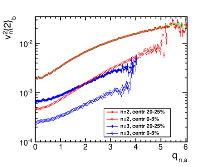
Figure 1: (color online) Mean elliptic and triangular flow values in $a$-subevent as function of the corresponding $q_{n}$ magnitude in $b$-subevent.

Zero nonflow. We start the discussion of the ESE with the simplest case when all the correlations in the system are determined only by anisotropic flow. Figure 1 shows the average values of $v_{n}^{2}$ calculated via 2-particle correlation method in one of the subevent (“b”) as function of the flow vector magnitude in the second subevent (“a”). We remind the reader, that in this simulations the two subevents are statistically independent and are correlated only via common participant plane and flow values. There are no nonflow correlations included at this stage. In this case the results for $v^{2}_{n,b}\{2\}$ coincide with “true” values of $\left\langle v^{2}_{n}\right\rangle$ (not shown), though have slightly larger statistical errors due to finite multiplicity of the subevent.

The results in Fig. 1 demonstrate, that depending on $q_{2,a}$ one can select events with average flow values varying more than a factor of two. How well one can “resolve” the flow fluctuations depends on the number of particles used to calculate the flow vector as well as, though weakly, on flow magnitude itself. We find that for centrality 20–25%, the width of the $v_{2}$ distribution for a fixed $q_{2,a}$ value is about factor of 1.5 smaller than that for unbiased event sample (changing from 0.031 to 0.022); it decreases for about 20% if one double the size of the subevent (double the multiplicity) used for $q_{2}$ determination.

Let us demostrate now how in practice one can obtain an information about the $v_{n}$ distributions, corresponding to different cuts on the $q_{n,a}$ values, from the fits to the $q_{n,b}$-distributions. Figure 2 shows distribution in $q_{n,b}$ (subevent-b) for three different cuts on $q_{n,a}$, separately for the second and third harmonic flow.

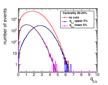
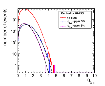
Figure 2: (color online) $q_{2,b}$ and $q_{3,b}$ distributions in the event samples selected by different cuts on the corresponding $q_{n,a}$-vector magnitude indicated in the plot. The lines show the BG fit to the distribution.

All $q_{n,b}$ distributions in Fig. 2 are fit to the BG functional form to extract the corresponding mean flow values and the corresponding width (see, e.g.  Voloshin:2008dg ). It is remarkable that the fits are very good not only for the unbiased $q$-distributions but also to the ones corresponding to the low flow and high flow “engineered events” (corresponding to the 5% lowest and 5% highest $q_{n,a}$ events). Using the extracted parameters we plot the corresponding $v_{n}$ distributions in Fig. 3 (shown by dashed lines) and compare to the actual (“true”) $v_{n}$ distributions, which is known in this Monte-Carlo simulation (shown as a histogram). One finds an excellent agreement between the two indicating that the $v_{n}$ distributions in the “shape engineered” events are very close to the BG form.

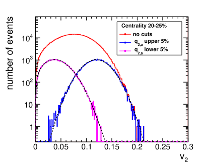
Figure 3: (color online) Actual (true) $v_{2}$ and $v_{3}$ distributions in the event samples selected by different cuts on the corresponding $q_{n}$-vector magnitude indicated in the plot compared to that extracted from the BG fits to $q_{n,b}$ distribution shown in Fig. 2 (dashed lines). Note that the lines are not the fit to the histograms!

Nonflow effects. The ESE approach described above is based on using two subevents. In this case possible nonflow effects can be separated in two major categories (a) when nonflow effects are present within each of the subevents, but there is no nonflow correlations between subevents “a” and “b”, and (b) when nonflow correlations are present between, as well as within, subevents. As we show below one should try to minimize the nonflow correlations between the two subevents which are used for ESE selection and physical analisys, respectively. A practical solution to that might be to use subevents which are separated by a significant (pseudo)rapidity gap.

The case (a) does present a certain challenges to the analysis, but no more than the one in the conventional flow analysis. Once the event selection is done with $q_{n,a}$ cuts, the flow in the selected events can be estimated using particles in subevent “b” with standard methods including many-particle cumulant analysis. The case (b) is significantly more complicated. Below we only discuss possible biases, without trying to resolve the problem.

We simulate nonflow effect by assuming that half of all particles in the entire event are produced in pairs with both particle in a pair emitted with the same azimuthal angle. Each particle is assigned randomly to one of the two subevents. In this case the nonflow parameter $\delta=1/(2M)$, where $M$ is the (full) event multiplicity, which roughly corresponds to the nonflow estimates in real LHC events for particles at midrapidity $|\eta|<0.8$.

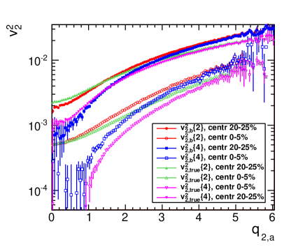
Figure 4: (color online) Elliptic flow measured with 2- (red points) and 4-particle (blue) cumulant method in subevent “a” as a function of the corresponding $q_{2,b}$ magnitude. Solid symbols correspond to centrality 20-25%, and open symbols to 0-5% centrality. The true (simulated) values are shown by green markers, as expected for 2-particle cumulant results and by magenta for 4-particle cumulant results.

Figure 4 presents the results for flow calculation in subevent “a” using 2- and 4-particle cumulant methods as function of $q_{2,b}$. The expectations based on simulated flow are also shown. One observes a significant bias due to nonflow, leading to overestimate the flow values in high flow selected events and underestimate in the low flow selected events. This trend is due to positive character of the nonflow correlations. The corresponding bias in corresponding $v$ distributions is shown in Fig. 5. Note that even though the bias for mean values of flow is somewhat modest, at large values of $v_{n}$ the actual distribution could differ by order of magnitude from the one deduced from $q$-distribution fits.

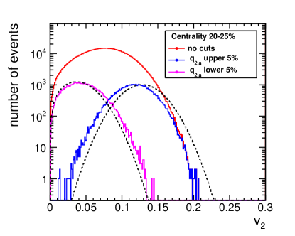
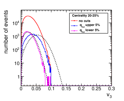
Figure 5: (color online) The same as in Fig 3 but for the case of nonflow described in text.

Below we discuss very briefly several analyses, which can profit from the event shape engineering.

The chiral magnetic effect proposed in Kharzeev:2004ey ; Kharzeev:2007tn ; Kharzeev:2007jp is a charge separation along the magnetic field. A correlator sensitive to the CME was proposed in Ref. Voloshin:2004vk :

$$\left\langle\cos(\phi_{\alpha}+\phi_{\beta}-2\Psi_{RP})\right\rangle,$$ (9)

where subscripts $\alpha,\;\beta$ denotes the particle type. The STAR :2009uh ; :2009txa , as well as the ALICE Abelev:2012pa collaboration measurements of this correlator are consistent with the expectation for the CME and can be considered as evidence of the local strong parity violation. The ambiguity in the interpretation of experimental results comes from a possible background of (the reaction plane dependent) correlations not related to CME. Note that a key ingredient to CME is the strong magnetic field, while all the background effects originate in the elliptic flow Voloshin:2004vk . This can be used for a possible experimental resolution of the question. One possibility is to study the effect in central collisions of non-spherical uranium nuclei Voloshin:2010ut , where the relative contributions of the background (proportional to the elliptic flow) and the CME (proportional to the magnetic field), should be very different in the tip-tip and body-body type collisions. The second possibility would be to exploit the large flow fluctuations in heavy-ion collisions as discussed in Voloshin:2010ut ; Bzdak:2011my and the ESE would be a technique to perform such an analysis. (Note also that the magnetic field depends very weakly on the initial shape geometry fluctuations Bzdak:2011my .) Yet another test, proposed in Voloshin:2011mx , is based on the idea that the CME, the charge separation along the magnetic field, should be zero if measured with respect to the 4-th harmonic event planes, while the background effects due to flow should be still present, albeit smaller in magnitude ($\sim v_{4}$). An example of such a correlator, would be $\left\langle\cos(2\phi_{\alpha}+2\phi_{\beta}-4\Psi_{4}\right\rangle$, where $\Psi_{4}$ is the fourth harmonic event plane. The value of the background due to flow could be estimated by rescaling the correlator Eq. 9. Such measurements will require good statistics, and strong fourth harmonic flow. Again, the ESE can be very helpful to vary the effects related to flow.

Measuring the shape and freeze-out velocity profile with azimuthally sensitive femtoscopy. Different shapes in the initial geometry of the collision, to a different degree will be preserved in the system freeze-out shapes. It was shown in Voloshin:2011mg that those shapes can be addressed experimentally with azimuthally sensitive femtoscopic analysis Voloshin:1995mc ; Voloshin:1997jh , which has a goal to obtain the geometry of the source relative to different harmonic symmetry planes. Such an analysis would definitely profit from event with extreme values of anisotropy provided by the ESE, as the variation of femtoscopic parameters with azimuth would be better pronounced. General details of femtoscopic analyses and discussion of the experimental results can be found in a review Lisa:2005dd .

Summary. Event shape engineering, providing possibility to study events corresponding to nuclear collisions with different initial geometry configuration, promises wide use in further studies of the properties of the strongly interacting matter.

I acknowledgements

The authors are indebted to our colleagues at the ALICE Collaboration for numerous fruitful discussion.

References

- (1)
- (2) S. A. Voloshin, A. M. Poskanzer and R. Snellings, in Landolt-Boernstein, Relativistic Heavy Ion Physics, Vol. 1/23, p 5-54 (Springer-Verlag, 2010)
- (3) B. Muller, J. Schukraft and B. Wyslouch, arXiv:1202.3233 [hep-ex].
- (4) A. P. Mishra, R. K. Mohapatra, P. S. Saumia, A. M. Srivastava, Phys. Rev. C77, 064902 (2008)
- (5) P. Sorensen, arXiv:0905.0174 [nucl-ex].
- (6) J. Takahashi et al., Phys. Rev. Lett. 103, 242301 (2009)
- (7) B. Alver and G. Roland, Phys. Rev. C 81, 054905 (2010) [Erratum-ibid. C 82, 039903 (2010)]
- (8) D. Teaney and L. Yan, arXiv:1010.1876 [nucl-th]
- (9) K. Aamodt et al. [ALICE Collaboration], Phys. Rev. Lett. 105, 252302 (2010)
- (10) K. Aamodt et al. [ALICE Collaboration], Phys. Rev. Lett. 107, 032301 (2011) [arXiv:1105.3865 [nucl-ex]]. G. Aad et al. [ATLAS Collaboration], Phys. Rev. C 86, 014907 (2012) [arXiv:1203.3087 [hep-ex]]. A. Adare et al. [PHENIX Collaboration], Phys. Rev. Lett. 107, 252301 (2011) [arXiv:1105.3928 [nucl-ex]]. M. Issah [CMS Collaboration], AIP Conf. Proc. 1422, 50 (2012). P. Sorensen [STAR Collaboration], J. Phys. G G 38, 124029 (2011) [arXiv:1110.0737 [nucl-ex]].
- (11) J. Adams et al. [STAR Collaboration], Phys. Rev. Lett. 95, 152301 (2005) [nucl-ex/0501016].
- (12) A. Adare et al. [PHENIX Collaboration], Phys. Rev. C 78, 014901 (2008) [arXiv:0801.4545 [nucl-ex]].
- (13) S. A. Voloshin, Phys. Rev. Lett. 105, 172301 (2010) [arXiv:1006.1020 [nucl-th]].
- (14) S. Voloshin and Y. Zhang, Z. Phys. C 70 665 (1996)
- (15) A. M. Poskanzer and S. A. Voloshin Phys. Rev. C 58 1671 (1998)
- (16) S. A. Voloshin, A. M. Poskanzer, A. Tang and G. Wang, Phys. Lett. B 659, 537 (2008) [arXiv:0708.0800 [nucl-th]].
- (17) K. Aamodt et al. [ALICE Collaboration], Phys. Rev. Lett. 106, 032301 (2011) [arXiv:1012.1657 [nucl-ex]].
- (18) J. Adams et al. [STAR Collaboration], Phys. Rev. C 72, 014904 (2005) [arXiv:nucl-ex/0409033].
- (19) P. Sorensen [STAR Collaboration], J. Phys. G G 35, 104102 (2008) [arXiv:0808.0356 [nucl-ex]].
- (20) D. Kharzeev, Phys. Lett. B 633, 260 (2006).
- (21) D. Kharzeev and A. Zhitnitsky, Nucl. Phys. A 797, 67 (2007).
- (22) D. E. Kharzeev, L. D. McLerran and H. J. Warringa, Nucl. Phys. A 803, 227 (2008).
- (23) S. A. Voloshin, Phys. Rev. C 70, 057901 (2004).
- (24) B. I. Abelev et al. [STAR Collaboration], Phys. Rev. Lett. 103, 251601 (2009).
- (25) B. I. Abelev et al. [STAR Collaboration], Phys. Rev. C 81, 054908 (2010).
- (26) B. Abelev et al. [ALICE Collaboration], arXiv:1207.0900 [nucl-ex].
- (27) A. Bzdak, arXiv:1112.4066 [nucl-th].
- (28) S. A. Voloshin, Prog. Part. Nucl. Phys. 67, 541 (2012) [arXiv:1111.7241 [nucl-ex]].
- (29) S. A. Voloshin, J. Phys. G 38, 124097 (2011) [arXiv:1106.5830 [nucl-th]].
- (30) S. A. Voloshin and W. E. Cleland, Phys. Rev. C 53, 896 (1996) [nucl-th/9509025]; Phys. Rev. C 54, 3212 (1996) [nucl-th/9606033].
- (31) S. Voloshin, R. Lednicky, S. Panitkin and N. Xu, Phys. Rev. Lett. 79, 4766 (1997) [nucl-th/9708044].
- (32) M. A. Lisa, S. Pratt, R. Soltz, U. Wiedemann, Ann. Rev. Nucl. Part. Sci. 55, (2005) 357