Leader Election and Gathering for Asynchronous Transparent Fat Robots without Chirality

Abstract

Gathering of autonomous mobile robots is a well known and challenging research problem for a system of multiple mobile robots. Most of the existing works consider the robots to be dimensionless or points. Algorithm for gathering fat robots (a robot represented as a unit disc) has been reported for three and four robots. This paper proposes a distributed algorithm which deterministically gathers $n$ $(n\geq 5)$ asynchronous, fat robots. The robots are assumed to be transparent and they have full visibility. Since the robots are unit discs, they can not overlap; we define a gathering pattern for them. The robots are initially considered to be stationary. A robot is visible in its motion. The robots do not store past actions. They are anonymous and can not be distinguished by their appearances and do not have common coordinate system or chirality. The robots do not communicate through message passing.

In the proposed gathering algorithm one robot moves at a time towards its destination. The robot which moves, is selected in such a way that, it will be the only robot eligible to move, until it reaches its destination. In case of a tie, this paper proposes a leader election algorithm which produces an ordering of the robots and the first robot in the ordering becomes the leader. The ordering is unique in the sense that, each robot, characterized by its location, agrees on the same ordering. We show that if a set of robots can be ordered then they can gather deterministically. The paper also characterizes the cases, where ordering is not possible.

This paper also presents an important fact that, if leader election is possible then gathering pattern formation is possible even with no chirality. It is known that, pattern formation and leader election are equivalent, for $n\geq 4$ robots when the robots agree on chirality. This paper proposes an algorithm for formation of the gathering pattern for transparent fat robots without chirality.

1 Introduction

A Robot Swarm [peleg2005, peleg2009] is a system of multiple autonomous mobile robots engaged in some collective task. In hostile environments, it may be desirable to employ large groups of low cost robots to perform various tasks cooperatively. This approach is more resilient to malfunction and more configurable than a single high cost robot. Swarm robotics, pioneered by C. W. Reynolds [reynolds1987], is a novel approach to coordinate a large number of robots. The idea is inspired by the observation of social insects. They are known to coordinate their actions to execute a task that is beyond the capability of a unit.

The field of swarm robotics has been enriched by many researchers adopting different approaches for swarm aggregation, navigation, coordination and control. Mobile robots can move in the physical world and interact with each other. Geometric problems are inherent to such multiple cooperative mobile robot systems and have been well studied [acm2004, IEEEJOR1999, celi2003, celi2002, cohen2004, cohen2005, disc2010, flocchini2001, gordon2008, peleg2005, prencipe2007]. Multiple robot path planning, moving to (and maintaining) formation and pattern generation are some important geometric problems in swarm robotics. Multiple robot path planning may deal with problems like finding non-intersecting paths for mobile robots [Fuj91]. The formation and marching problems require multiple robots to form up and move in a specified pattern. These problems are also interesting in terms of distributed algorithms. Formation and marching problems may act as useful primitives for larger tasks, like, moving a large object by a group of robots [SB93] or distributed sensing [WB88]. Pattern generation in Cellular Robotic Systems (CRS) [ben1988] is related to pattern formation problem by mobile robots.

This paper addresses a very well known and challenging problem involving robot swarms, namely Gathering. The objective is to collect multiple autonomous mobile robots into a point or a small region. The choice of the point is not fixed in advance. Initially the robots are stationary and in arbitrary positions. Gathering problem is also referred to as Point Formation, Convergence, Homing or Rendezvous [prencipe2006].

2 Earlier Works

A pragmatic view of swarm robots asks for distributed environment. Several interesting works have been carried out by researchers [acm2004, cohen2004, peleg2009, flocchini2000, gordon2008, katayama2007, klasing2006] on distributed algorithms for mobile robots. A simple basic model called weak model [peleg2007, prencipe2006] is popular in the literature. The world of the robots consists of the infinite plane and multiple robots living on it. The robots were considered dimensionless or points. All robots are autonomous, homogeneous and perform the same algorithm (Look-Compute-Move cycle) [peleg2007]. In look state, a robot takes a snapshot of its surroundings, within its range of vision. It then executes an algorithm for computing the destination in compute state. The algorithm is same for all robots. In move state, the robot moves to the computed destination. The robots are oblivious (memoryless). They do not preserve any data computed in the previous cycles. There is no explicit communication between the robots. The robots coordinate by means of observing the positions of the other robots on the plane. A robot is always able to see another robot within its visibility radius or range (may be infinite). Two different models have been used for robots’ movement [prencipe2001]. Under the SYM model, the movement of a robot was considered to be instantaneous, i.e., when a robot is moving, other robots can not see it. Later, that model has been modified to CORDA model where the movement of a robot is not instantaneous. A robot in motion is visible. The CORDA model is a better representation of the real world. The robots may or may not be synchronized. Synchronous robots execute their cycles together. In such a system, all robots get the same view. As a result, they compute on same data. In the more practical asynchronous model, there is no such guarantee. By the time a robot completes its computation, several of the robots may have moved from the positions based on which the computation is made. The robots may have a common coordinate system or individual coordinate systems having no common orientation or scale [peleg2007].

The problem of gathering multiple robots has been studied on the basic model of robotic system with different additional assumptions. Prencipe [prencipe2007] observed that gathering is not always possible for asynchronous robots. However, instead of meeting at a single point, if the robots are asked to move very close to each other, then the problem can be solved by computing the center of gravity of all robots and moving the robots towards it. Under the weak model, robots do not have any memory. As they work asynchronously and act independently, once a robot moves towards the center of gravity, the center of gravity also changes. Moving towards center of gravity does not gather robots to a single point. However, this method makes sure that the robots can be brought as close as one may wish.

A possible solution to this problem is to choose a point which, unlike center of gravity, is invariant with respect to robots’ movement. One such point in the plane is the point which minimizes the sum of distance between itself and all the robots. This point is called the Weber or Fermat or Torricelli point. It does not change during the robots’ movement, if the robots move only towards this point. However, the Weber point is not computable for higher number of robots (greater than 4) [bajaj1988]. Thus, this approach also can not be used to solve the gathering problem. If common coordinate system is assumed, instead of individual coordinate systems, then the Gathering problem is solvable even with limited visibility [flocchini2001]. If the robots are synchronous and their movements are instantaneous, then the gathering problem is solvable even with limited visibility [IEEEJOR1999]. Cieliebak et al. [celi2003], show that there are solutions for gathering without synchronicity if the visibility is unlimited. One approach is by multiplicity detection. If multiple robots are at the same point then the point is said to have strict multiplicity. However, the problem is not solvable for two robots even with multiplicity detection [prencipe2007]. There are some solutions for three and four robots. For more than four robots, there are two algorithms with restricted sets of initial configurations [celi2002]. In the first algorithm, the robots are initially in a bi-angular configuration. In such a configuration, there exists a point $c$ and two angles $a$ and $b$ such that the angle between any two adjacent robots is either $a$ or $b$ and the angles alternate. The second algorithm works if the initial configuration of the robots do not form any regular $n$-gon. Prencipe [prencipe2007] reported that there exists no deterministic oblivious algorithm that solves the gathering problem in a finite number of cycles for a set of $n\geq 2$ robots. Convergence of multiple robots is studied by Peleg and Cohen [cohen2005] and they proposed a gravitational algorithm in fully asynchronous model for convergence of any number of robots.

A dimensionless robot is unrealistic. Czyzowicz et al.,[czy2009] extend the weak model by replacing the point robots by unit disc robots. They called these robots as fat robots. The methods of gathering of three and four fat robots have been described by them. The paper considers partial visibility and presents several procedures to avoid different situations which cause obstacles to gathering. We proposed a deterministic gathering algorithm for $n$ $(n\geq 5)$ fat robots [km2010]. The robots are assumed to be transparent in order to achieve full visibility.

Having fat robots, we first define the gathering pattern to be formed by the robots. Therefore, gathering pattern formation becomes a special case of pattern formation of mobile robots which is also a challenging problem for mobile robots. Recent works [disc2010, dieu2010] shows that pattern formation and leader election are equivalent for $n\geq 4$ robots. However, this work [disc2010] considered the robots to have common handedness or chirality. We propose a gathering algorithm which assumes no chirality and use the leader election technique in order to form gathering pattern. We also show that if leader election is possible then formation of the gathering pattern is possible even with no chirality. Section 3 describes the model used in this paper and presents an overview of the problem. Then we move to the solution approach. Section 4 characterizes the geometric configurations of the robots for gathering. Section 5 presents the leader election and gathering algorithms. Finally section LABEL:con summarizes the contributions of the paper and concludes.

3 Robot Model and Overview of the Problem

We use the basic structure of weak model [peleg2007, prencipe2006] and add some extra features which extend the model. Let $R=\{r_{1},r_{2},\ldots,r_{n}\}$ be a set of fat robots. A robot is represented by its center, i.e., by $r_{i}$ we mean a robot whose center is $r_{i}$. The following assumptions describe the system of robots deployed on the 2D plane:

• Robots are autonomous.

• Robots execute the cycle (Look-Compute-Wait-Move) asynchronously.

• Robots are anonymous and homogeneous in the sense that they are not uniquely identifiable, neither with a unique identification number nor with some external distinctive mark (e.g., color, flag, etc.).

• A robot can sense all other robots irrespective of their configuration.

• Each robot is represented as a unit disc (fat robots).

• CORDA [prencipe2001] model is assumed for robots’ movement. Under this model the movement of the robots is not instantaneous. While in motion, a robot may be observed by other robots.

• Robots have no common orientation or scale. Each robot uses its own local coordinate system (origin, orientation and distance). A robot has no particular knowledge about the coordinate system of any other robot, nor of a global coordinate system.

• Robots can not communicate explicitly. Each robot has a camera or sensor which can take picture or sense over 360 degree. The robots communicate only by means of observing other robots using the camera or sensor. A robot can compute the coordinates (w.r.t. its own coordinate system) of other robots by observing through the camera or sensor.

• Robots have infinite visibility range.

• Robots are assumed to be transparent to achieve full visibility.

• Robots are oblivious. They do not remember the data from the previous cycles.

• Initially all robots are stationary.

Let us define the Gathering Pattern which is to be formed by $R$.

The desired gathering pattern for transparent fat robots is shown in Fig. 1(a). One robot with center $C$ is at the center of the structure. We call it layer $0$. Robots at layer $1$ are around layer $0$ touching $cir(C,1)$ ($cir(a,n)$ is a circle with center at $a$ and radius $n$). Robots at layer $2$ are around layer $1$ touching $cir(C,3)$ and so on. Fig. 1(a) shows a gathering pattern with $3$ layers.

Figure 1: Gathering pattern of multiple robots

Definition 1

Gathering pattern is a circular layered structure of robots with a unique robot centered at $C$. A robot at layer $\ell+1$ touches $cir(C,2\ell+1)$ and at least $1$ and at most $2$ robots at layer $\ell+1$. The inner layers are full. The outer most layer may not be full but the vacant places in the outer most layers must be contiguous.

According to the definition, a unique center is required to form a gathering pattern and the layers are created around the center. Finding a unique robot and marking it as the center is not possible for $2$, $3$ and $4$ robots. This is due to the symmetric structure (Fig. 2). For 2 or 3 robots all robots are potential candidates to be the center. For 4 robots there are two such robots. To identify a unique robot for the center of the gathering pattern, at least $5$ robots are required. For $5$ robots, a robot which touches the rest $4$ robots is treated as the central robot or a robot at layer $0$. Fig. 1(b) shows the desired gathering pattern with minimum robots.

Figure 2: Gathering of 2, 3 and 4 robots

We are given a set, $R$, of separated, stationary transparent fat robots. The objective is to move the robots so as to build the gathering pattern with the robots in $R$. For gathering multiple robots, our approach is to select one robot and assign it a destination. All other robots remain stationary till the designated robot reaches its destination. At each turn, the robot selected for motion is chosen in such a way, that during the motion if any other robot takes a snapshot and computes, this particular robot would be the only one eligible for movement. To implement this, we choose a destination carefully. The robot, nearest to the destination, is allowed to move first. However, a problem will occur when multiple robots are at same distance from the destination. A leader election mechanism is required to select a robot among such multiple eligible robots. To overcome this problem, our approach is to order a set of robots on 2D plane, with respect to the destination. The robots move one by one, according to this order, towards the destination. The mutual ordering of the robots in the set is invariant, though the size of the set changes.

4 Characterization of the Geometric Configurations of Robots for Gathering

A set of robots on 2D plane is given. Our objective is to move them, one by one, to form desire gathering pattern. In order to do so, we create an ordering among the robots and move one by one following the ordering. This ordering will be computed at different robot sites, who have different coordinate systems, orientations and origins. Thus, we need the ordering algorithm to yield the same result, even if the point set is given a transformation with respect to origin, axes and scale. For this to succeed, no two robots should have the same view. Keeping this in mind, we proceed to characterize the geometric configurations that is required for a set of robots to be orderable (formal definition is presented shortly). In this section we represent the robots by points.

Let $P=\{p_{1},p_{2},\ldots,p_{n}\}$ be a non-empty set of points on the 2D plane. $\cal L$ is a line on the plane. Let $P_{\cal L}\subset P$ be the points of $P$ (not all), which lie on $\cal L$. $\cal L$ partitions $P\setminus P_{\cal L}$ into two subsets $H$ and $H^{\prime}$ where $H$ or $H^{\prime}$ is non-empty. Let $\cal L^{\prime}$ be the straight line that intersects $\cal L$ at point $m$ such that ${\cal L^{\prime}}\bot{\cal L}$ and $m$ is the middle point of the span of the points on $P_{\cal L}$.

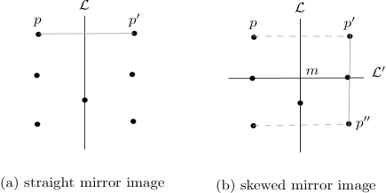
Figure 3: Examples of straight and skewed mirror images.

Definition 2

A point $p^{\prime}\in P$ is said to be a straight mirror image of $p\in P$ across $\cal L$, if $p^{\prime}$ is a mirror image of $p$ across $\cal L$ (Figure 3(a)).

Definition 3

Let $p^{\prime}$ be the straight mirror image of $p$ across $\cal L$. $p^{\prime\prime}$ is the straight mirror image of $p^{\prime}$ across $\cal L^{\prime}$. $p^{\prime\prime}$ is said to be skewed mirror image of $p$ across $\cal L$ (Figure 3(b)).

Definition 4

A set of points $P$ on the 2D plane is said to be in straight-symmetric configuration, if there exists a straight line $\cal L$ (on that plane) not containing all the points of $P$, such that each point in $H\cup P_{\cal L}$ has a straight mirror image in $H^{\prime}\cup P_{\cal L}$ (Figure. 4(a)). The line $\cal L$ is called a line of straight symmetry.

Figure 4: Examples of straight and skew symmetric configurations.

Note that each point in $P_{\cal L}$ is the mirror image of itself.

Definition 5

A set of points $P$ on the 2D plane is said to be in skew-symmetric configuration, if there exists a straight line $\cal L$ (on that plane) not containing all the points of $P$, such that each point in $H\cup P_{\cal L}$ has a skewed mirror image in $H^{\prime}\cup P_{\cal L}$. (Figure. 4(b)). The line $\cal L$ is called a line of skew symmetry.

Definition 6

A set of points $P$ on the 2D plane is said to be in symmetric configuration (denoted by $\O{}_{S}$), if it is either a singleton set or in straight symmetric or skew symmetric configuration. For a singleton set, any line passing through the point is a line of symmetry.

Definition 7

A set of points $P$, which is not in symmetric configuration is in asymmetric configuration (denoted by $\O{}_{A}$).

Our requirement does not stop at requiring the algorithm to be robust to changes in the coordinate system. The positions of the robots also change as the algorithm progresses. Our objective is to order the points (robots) in $P$ such that when the robots move one by one, according to this order, towards the destination, the mutual ordering of the robots in the set is invariant. We define an orderable set as follows.

Definition 8

A set of points $P$, on the plane, is called an orderable set, if there exists a deterministic algorithm, which produces a unique ordering of the points of $P$, such that the ordering is same irrespective of the choice of origin and coordinate system.

Lemma 1

Let $P$ be a non-empty, non-singleton set of points. If $P$ is in $\O{}_{s}$, then $P$ is not orderable.

Proof: Let $\cal L$ be a line of symmetry (straight or skewed) for $P$. Let $P_{\cal L}$ be the set of points from $P$, lying on $\cal L$. $\cal L$ divides $P\setminus P_{\cal L}$ into two halves $H$ and $H^{\prime}$. $H\cup P_{\cal L}$ and $H^{\prime}\cup P_{\cal L}$ are mirror images (straight or skewed) of each other. Let $p_{i}$ be a point in $H$ and $p^{\prime}_{i}$ in $H^{\prime}$, the mirror image of $p_{i}$. Consider an arbitrary ordering algorithm $\cal A$. If we run $\cal A$ on $P$ with $p_{i}$ as the origin, it produces an ordering of $P$. Let $p_{j}$ be the first point from that ordering such that $p_{j}$ is not on $P_{\cal L}$. On the other hand, if we run $\cal A$ on $P$, with $p^{\prime}_{i}$ as the origin, the symmetry tells us that the ordering obtained will have $p^{\prime}_{j}$ (the mirror image of $p_{j}$) as the corresponding first point in the order. Since, $p_{j}$ is not in $P_{\cal L}$, $p_{j}\neq p^{\prime}_{j}$. Since the choice of $\cal A$ was arbitrary, no algorithm will produce the same order irrespective of the choice of origin. Hence, $P$ is not orderable.

Observation 1

Any line of symmetry of $P$ passes through the center of the Smallest Enclosing Circle (SEC) of $P$ and divides the points on SEC into two equal mirror images (straight or skewed).

In order to check whether a set of points is in $\O{}_{s}$ or not, we need to find out if a line of symmetry exists for this set. For this search to be feasible, we need to reduce the potential set of candidate lines for line of symmetry. In order to do so, first the SEC of $P$ is computed. The points on the SEC are taken to form a convex polygon, say ${\cal H}(P)$.

Observation 2

A line of symmetry (straight or skewed) of $P$ cuts ${\cal H}(P)$ at two points. Thus the line of symmetry contains at most two points from ${\cal H}(P)$.

Lemma 2

Let $P$ be a set of points in $\O{}_{s}$. The mirror image (straight or skewed) of a vertex in $\cal H$ is also in ${\cal H}(P)$.

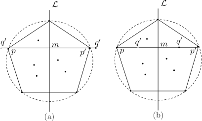
Figure 5: The mirror image of a hull vertex is also a hull vertex.

Proof: Consider a vertex $p$ of ${\cal H}(P)$. Let $p^{\prime}$ be the mirror image of $p$ across the line of symmetry $\cal L$. Suppose, $p^{\prime}$ is not in ${\cal H}(P)$. Suppose, the line $pp^{\prime}$ intersects ${\cal L}$ at $m$ and intersects ${\cal H}(P)$ at $q$. $\overline{pm}=\overline{mp^{\prime}}$ . $q$ should also have a mirror image across $\cal L$, in the same side where $p$ lies. Let $q^{\prime}$ be the mirror image of $q$. Note that $qq^{\prime}$ also intersects $\cal L$ at point $m$ and $\overline{qm}=\overline{mq^{\prime}}$. If $p^{\prime}$ is inside the convex hull then $\overline{mp^{\prime}}<\overline{mq}$ (Figure. 5(a)). Hence, $\overline{mp}<\overline{mq}$ and $\overline{mp}<\overline{mq^{\prime}}$. This implies that $p$ is not a hull vertex. Contradiction! On the other hand, if $p^{\prime}$ is outside the convex hull then $\overline{mp^{\prime}}>\overline{mq}$ (Figure. 5(b)). Hence, $\overline{mp}>\overline{mq}$ and $\overline{mp}>\overline{mq^{\prime}}$. This implies that $p$ is not a hull vertex. Contradiction! Therefore, if $p$ is a hull vertex, $p^{\prime}$ must also be a hull vertex.

Lemma 3

If $P$ is in $\O{}_{s}$, then ${\cal H}(P)$ is in $\O{}_{s}$.

Proof: Follows from lemma 2.

Lemma 4

If ${\cal H}(P)$ is in $\O{}_{S}$, then for any line of straight symmetry $\cal L$ of $P$,

1. if $\cal L$ passes through a vertex $v$ of ${\cal H}(P)$, it bisects the interior angle at $v$,

2. if $\cal L$ intersects an edge $e$ of ${\cal H}(P)$, at a point other than a vertex, it is the perpendicular bisector of $e$.

Proof: Follows from the proof of lemma 2.

Observation 3

Any line of skew symmetry intersects ${\cal H}(P)$ either at two vertices or at two edges.

Observation 4

A skew symmetric polygon has even number of vertices and edges.

Lemma 5

A pair of edges in a polygon inscribed in a circle is parallel and equal if and only if they are opposite sides of a unique rectangle inscribed in that circle.

Figure 6: A pair of parallel and equal edges of a polygon forms a rectangle.

Proof:

If: Trivial.

Only if: Suppose $P_{k}P_{k+1}$ and $P_{l}P_{l+1}$ are two edges of a polygon such that $\overline{P_{k}P_{k+1}}=\overline{P_{l}P_{l+1}}$ and $P_{k}P_{k+1}||P_{l}P_{l+1}$ (Fig. 6). $C$ is the intersection point of the lines $P_{k}P_{l}$ and $P_{k+1}P_{l+1}$. It is easy to see that $\triangle P_{k}CP_{k+1}\cong\triangle P_{l}CP_{l+1}$. So, $\overline{P_{k+1}C}=\overline{P_{l+1}C}$ and $\overline{P_{k}C}=\overline{P_{l}C}$. This means that the cords, $P_{k}P_{l}$ and $P_{k+1}P_{l+1}$ bisect each other. Hence, $P_{k}P_{l}$ and $P_{k+1}P_{l+1}$ are both diameters of the circle. Therefore, $\overline{P_{k}P_{l}}=\overline{P_{k+1}P_{l+1}}$. This implies that $P_{k}P_{k+1}P_{l}P_{l+1}$ is a rectangle.

Figure 7: A pair of parallel and equal edges of a polygon forms rectangles.

Lemma 6

A polygon ${\cal H}(P)$, inscribed in a circle, is skew symmetric if and only if each edge of the polygon has a parallel edge of equal length.

Proof: If: Suppose $P_{k}P_{k+1}$ and $P_{l}P_{l+1}$, are parallel and equal edges of ${\cal H}(P)$ (Fig 7). Let us add $P_{k+1}$ and $P_{l+1}$ by a straight line $\cal L$. We shall show that $\cal L$ is a line of skew symmetry for ${\cal H}(P)$. $P_{l+1}P_{l}$ is the skewed mirror image of $P_{k}P_{k+1}$ across $\cal L$. Let $P_{k+1}P_{k+2}$ be the adjacent edge of $P_{k}P_{k+1}$. We add $P_{k+2}P_{l+1}$. Since, $P_{k+1}P_{l+1}$ is a diameter of the circumcircle of ${\cal H}(P)$ (lemma 5), $\angle P_{k+1}P_{k+2}P_{l+1}=90$ degree. We draw the rectangle $P_{k+1}P_{k+2}P_{l+1}P_{l+2}$. By lemma 5, $P_{l+1}P_{l+2}$ is the edge of the polygon which is parallel to and equal in length with $P_{k+1}P_{k+2}$. By repeating this argument it can be shown that, polygonal chains on both sides of $\cal L$ are skew symmetric.

Only if: Let ${\cal H}(P)$ be a skew symmetric polygon. $\cal L$ is a line of skew symmetry for ${\cal H}(P)$. $\cal L$ partitions ${\cal H}(P)$ into two halves namely, $H_{1}$ and $H_{2}$.

First consider the case when $\cal L$ passes through two vertices of ${\cal H}(P)$, namely $v_{\alpha}$ and $v_{\beta}$. (Fig 8). Suppose, $e_{1}$ is the edge incident at $v_{\alpha}$ in $H_{1}$ and $e_{2}$ is the edge incident at $v_{\beta}$ in $H_{2}$. Since, $\cal L$ is a line of skew symmetry, $e_{2}$ is the skewed mirror image of $e_{1}$. Therefore, $\overline{e_{1}}=\overline{e_{2}}$ and $e_{1}||e_{2}$. Let $f_{1}$ be the edge adjacent to $e_{1}$ in $H_{1}$ and $f_{2}$ the edge adjacent to $e_{2}$ in $H_{2}$. Similarly, $f_{2}$ is the mirror image of $f_{1}$. Therefore, $\overline{f_{1}}=\overline{f_{2}}$ and $f_{1}||f_{2}$. In this manner, we can find a parallel and equal edge of every edge.

Now consider the case when $\cal L$ intersects two edges of ${\cal H}(P)$, namely $e_{1}=p_{1}p_{2}$ and $e_{2}=q_{1}q_{2}$ at point $m_{1}$ and $m_{2}$ respectively (Fig 8). If we consider a modified polygon with additional vertices at $m_{1}$ and $m_{2}$, the result follows from the previous case.

Suppose, ${\cal H}(P)$ is a skew symmetric polygon. Let $\cal L$ be a line intersecting two vertices of ${\cal H}(P)$, namely $v_{\alpha}$ and $v_{\beta}$. Let $\alpha$ be the interior angle of ${\cal H}(P)$ at vertex $v_{\alpha}$ and $\beta$ be the interior angle of ${\cal H}(P)$ at vertex $v_{\beta}$. $\cal L$ divides $\alpha$ into ${\alpha}_{1}$ and ${\alpha}_{2}$ and $\beta$ into ${\beta}_{1}$ and ${\beta}_{2}$ (Fig 8). Suppose, $e_{1}$ is an edge incident at $v_{\alpha}$ in $H_{1}$ and $e_{2}$ is an edge incident at $v_{\beta}$ in $H_{2}$. $f_{1}$ is the edge adjacent to $e_{1}$ in $H_{1}$ and $f_{2}$ is the edge adjacent to $e_{2}$ in $H_{2}$.

Lemma 7

For a skew symmetric polygon ${\cal H}(P)$, $\cal L$ is a line of skew symmetry if and only if ${\alpha}_{1}={\beta}_{2}$ or ${\alpha}_{2}={\beta}_{1}$.

Proof: If: If ${\alpha}_{1}={\beta}_{2}$, $e_{1}||e_{2}$. From lemma 6, there exist an edge $e_{1}^{\prime}$ such that $e_{1}||e_{1}^{\prime}$ and $\overline{e_{1}}=\overline{e_{1}^{\prime}}$. As ${\cal H}(P)$ is convex $e_{1}||e_{1}^{\prime}$ and $e_{1}||e_{2}$ implies $e_{1}^{\prime}$ and $e_{2}$ are the same. Hence, $\overline{e_{1}}=\overline{e_{2}}$. Using an argument similar to that used in the proof of lemma 5, it can be shown that, polygonal chains on both sides of $\cal L$ are skew symmetric. Similarly, if ${\alpha}_{2}={\beta}_{1}$, polygonal chains on both sides of $\cal L$ are skew symmetric. Hence, $\cal L$ is a line of skew symmetry.

Only if: Follows from the definition of skew symmetric polygon.

Figure 8: Examples of skew symmetry in convex hull.

Let $\cal L$ be a line intersecting two edges of ${\cal H}(P)$, namely $e_{1}=p_{1}p_{2}$ and $e_{2}=q_{1}q_{2}$ at point $m_{1}$ and $m_{2}$ respectively (Fig 8).

Lemma 8

For a skew symmetric polygon ${\cal H}(P)$, $\cal L$ is a line of skew symmetry if and only if $e_{1}$ $||$ $e_{2}$, $\overline{p_{1}m_{1}}=\overline{m_{2}q_{2}}$ and $\overline{m_{1}p_{2}}=\overline{q_{1}m_{2}}$.

Proof: If: $e_{1}$ $||$ $e_{2}$, $\overline{p_{1}m_{1}}=\overline{m_{2}q_{2}}$ and $\overline{m_{1}p_{2}}=\overline{q_{1}m_{2}}$ implies that $q_{2}$ is the skewed mirror image of $p_{1}$ and $p_{2}$ is the skewed mirror image of $q_{1}$ across $\cal L$. As $\overline{e_{1}}=\overline{e_{2}}$, using an argument similar to that used in the proof of lemma 5, it can be shown that, polygonal chains on both sides of $\cal L$ are skew symmetric. Hence, $\cal L$ is a line of skew symmetry.

Only if: Follows from the definition of skew symmetric polygon.

In order to check whether a set of points $P$ is in $\O{}_{s}$ or not, we first compute the SEC of $P$. The convex polygon ${\cal H}(P)$, as described earlier, is also computed. For each vertex and each edge of ${\cal H}(P)$, we look for a line of symmetry $\cal L$ (straight or skewed) passing through that vertex or edge.

Since, we want the ordering to be the same for any choice of origin and axes, we can only use information which are invariant under these transformations. Examples of such properties are, distances and angles between the points. The distances may be affected by the choice of unit distance, but even then their ratios remain the same. One possible solution is to select the robot closest to the destination as the leader or the candidate to move. It also satisfies our extra requirement that it remains the point closest the destination, and hence the leader, as it moves. Robots equidistant from the destination are on the circumference of a circle with the destination as its center. They also form a convex polygon. Let $G$ be a set of robots forming such a convex polygon inscribed in a circle. For the rest of this paper, by convex polygon we mean such polygons which are inscribed in a circle. The center of the circle is called the center of the polygon.

Definition 9

A convex polygon $G$ is straight symmetric if the set of vertices in $G$ is in straight symmetric configuration.

Definition 10

A convex polygon $G$ is skew symmetric if the set of vertices in $G$ is in skew symmetric configuration.

Definition 11

A convex polygon $G$ is symmetric if it is either straight symmetric or skew symmetric.

Definition 12

A polygon, which is not symmetric is asymmetric.

Note: A single point on a circle is a special case. It is symmetric. Though, any line passing through it is a line of symmetry, we shall only call the line passing through the center of the circle (and the point itself) as the line of symmetry.

Observation 5

The set of vertices of an asymmetric polygon is in $\O{}_{A}$.

Figure 9: Any straight line passing through the center of a skew symmetric polygon, is a line of skew symmetry for that polygon

Lemma 9

Any straight line passing through the center of a skew symmetric polygon, is a line of skew symmetry for that polygon.

Proof: Let $G$ be a skew symmetric polygon. Let $v_{i}v_{j}$ and $v^{\prime}_{i}v^{\prime}_{j}$ be two parallel and equal length edges of $G$ (Figure. 9). Let ${\cal L}_{1}$ and ${\cal L}_{2}$ be the lines passing through $v_{i}$-$v^{\prime}_{j}$ and $v_{j}$-$v^{\prime}_{i}$ respectively. From lemma 5, it follows that ${\cal L}_{1}$ and ${\cal L}_{2}$ pass through the center $C$ of $G$ and they are lines of skew symmetry of $G$. Now it is sufficient to prove that any line passing through the center and intersecting $\overline{v_{i}v_{j}}$ is a line of skew symmetry for $G$. Without loss of generality let us rotate ${\cal L}_{1}$ by some angle, around $C$, keeping it between ${\cal L}_{1}$ and ${\cal L}_{2}$. Let ${\cal L}^{\prime}_{1}$ be the new position of the line. Following lemma 8 and using an argument similar to that used in the proof of lemma 5, it can be shown that, polygonal chains on both sides of ${\cal L}^{\prime}_{1}$ are skew symmetric. Hence, ${\cal L}^{\prime}_{1}$ is a line of skew symmetry.

For a convex polygon, a line of symmetry $\cal L$ (straight or skewed) intersects the polygon at two points. The points can be two vertices or they may lie on two edges or one point may be a vertex and the other point lies on an edge (Figure. 10). Let $\cal L$ intersect $G$ at $m$ and $m^{\prime}$. Suppose $G$ has $k$ vertices. The vertices are labeled starting from the vertex next (clockwise) to $m$ up to the previous vertex of $m$, as $v_{1},v_{2},\ldots,v_{n}$. If $m$ is a vertex, then $n=k-1$. If $m$ lies on an edge, $n=k$. Similarly, the vertices are labeled starting from the vertex next (clockwise) to $m^{\prime}$ up to the previous vertex of $m^{\prime}$, as $v^{\prime}_{1},v^{\prime}_{2},\ldots,v^{\prime}_{n^{\prime}}$. If $m^{\prime}$ is a vertex, then $n^{\prime}=k-1$. If $m^{\prime}$ lies on an edge, $n^{\prime}=k$.

The following notations are used in the rest of this paper.

• $CW_{m}=(\overline{mv_{1}},\overline{mv_{2}},\ldots,\overline{mv_{n}})$.

• $ACW_{m}=(\overline{mv_{n}},\overline{mv_{n-1}},\ldots,\overline{mv_{1}})$.

• $CW_{m^{\prime}}=(\overline{m^{\prime}v^{\prime}_{1}},\overline{m^{\prime}v^{\prime}_{2}},\ldots,\overline{m^{\prime}v^{\prime}_{n^{\prime}}})$.

• $ACW_{m^{\prime}}=(\overline{m^{\prime}v^{\prime}_{n^{\prime}}},\overline{m^{\prime}v^{\prime}_{n^{\prime}-1}},\ldots,\overline{m^{\prime}v^{\prime}_{1}})$.

$CW_{m}=ACW_{m}$ iff $\overline{mv_{i}}=\overline{mv_{n-i+1}}$ for ($1\leq i\leq n$).

Figure 10: Examples of symmetric polygons with line of symmetry intersecting the polygon by two vertices (a) and by two edges (b) and by one edge and one vertex (c).

Lemma 10

Let $G$ be a straight symmetric polygon. A straight line $\cal L$ is a line of straight symmetry for $G$ if and only if $CW_{m}=ACW_{m}$ or $CW_{m^{\prime}}=ACW_{m^{\prime}}$.

Proof: Follows from definition 4 and definition 9.

Lemma 11

Let $G$ be a skew symmetric polygon and $\cal L$ a line of skew symmetry. $\cal L$ divides $G$ into two skewed mirror image parts if and only if $CW_{m}=CW_{m^{\prime}}$ or $ACW_{m}=ACW_{m^{\prime}}$.

Proof: Follows from definition 5 and definition 10.

Theorem 1

A polygon $G$ is asymmetric if and only if all of the following conditions are true

1. $CW_{v_{i}}\neq ACW_{v_{i}}$ for $1\leq i\leq n$.

2. $CW_{v_{i}}\neq CW_{v_{j}}$ for $1\leq i,j\leq n$ and $i\neq j$.

3. $CW_{v_{i}}\neq ACW_{v_{j}}$ for $1\leq i,j\leq n$ and $i\neq j$

Note: $CW_{v_{i}}\neq CW_{v_{j}}$ and $ACW_{v_{i}}\neq ACW_{v_{j}}$ are equivalent. Theorem 1 can also be written as follows.

Theorem 1.1: A polygon $G$ is asymmetric if and only if all of the following conditions are true

1. $CW_{v_{i}}\neq ACW_{v_{i}}$ for $1\leq i\leq n$.

2. $ACW_{v_{i}}\neq ACW_{v_{j}}$ for $1\leq i,j\leq n$ and $i\neq j$.

3. $ACW_{v_{i}}\neq CW_{v_{j}}$. for $1\leq i,j\leq n$ and $i\neq j$

Lemma 12

An asymmetric polygon is orderable.

Proof: Let $G$ be an asymmetric polygon. For each vertex $v_{k}$ ($1\leq k\leq n$), we compute the tuple $\{CW_{v_{k}},ACW_{v_{k}}\}$ and take the lexicographic minimum of the $n$ tuples as the ordering of $G$. Since $G$ is asymmetric, $CW_{v_{i}}\neq ACW_{v_{i}}$ for any $v_{i}$ and $CW_{v_{i}}\neq CW_{v_{j}}$, $ACW_{v_{i}}\neq ACW_{v_{j}}$ for any $v_{i}$ and $v_{j}$ such that $i\neq j$ (theorem 1). Hence, the ordering is same irrespective of the choice of origin or the coordinate axes. Thus, the set of vertices of an asymmetric polygon is orderable (definition 8).

A set of points which are equidistant from the destination, form a convex polygon such that the vertices of the polygon are on the circumference of a circle. There can be multiple such sets, i.e., the robots within a set are equidistant from the destination but the robots in different sets are not equidistant from the destination. In such a case, we get multiple concentric circles each of them enclosing a convex polygon.

Let $\cal G$ = $(G_{1},G_{2},\ldots,G_{t})$, be the $t$ convex polygons whose union is the whole set of points. The vertices of each polygon in $\cal G$ are on the circumference of a circle. These circles are concentric. The center of the circles is known. Generally, the center $C$ is the center of the SEC formed by the points in $\cal G$. $C$ is also considered as the center of any polygon $G_{i}\in\cal G$. Elements of $\cal G$ are sorted according to their distances from the center. Any polygon $G_{i}\in\cal G$ can be extracted by selecting the equidistant points from the center. The polygon at level $1$ ($G_{1}$) is the closest and the polygon at level $t$ ($G_{t}$) is the farthest.

Definition 13

A pair of polygons $G_{i}$ and $G_{j}$(denoted by $<G_{i},G_{j}>$) in $\cal G$ is called a symmetric pair, if $G_{i}$ and $G_{j}$ have a common line of symmetry.

A pair is asymmetric if it is not symmetric.

Observation 6

If any of the polygons of a pair is asymmetric, then the pair is asymmetric.

Lemma 13

A symmetric pair is not orderable.

Proof: Suppose $<G_{i},G_{j}>$ is a symmetric pair. $G_{i}$ and $G_{j}$ have a common line of symmetry (straight or skewed) $\cal L$, which divides $G_{i}$ and $G_{j}$ into two equal halves (straight or skewed mirror image). The union of the vertices of $G_{i}$ and $G_{j}$ is divided into two equal halves by $\cal L$. The union of the vertices of $G_{i}$ and $G_{j}$ is in $\O{}_{S}$. Hence, $<G_{i},G_{j}>$ is not orderable (lemma 1).

Suppose, the vertices of $G_{i}$ in pair $<G_{i},G_{j}>$ are projected radially on the circumference of the enclosing circle of $G_{j}$ ($i<j$). Construct a polygon $G_{ij}$ with the full set of vertices on the circle.

Observation 7

If $<G_{i},G_{j}>$ is an asymmetric pair, then the polygon $G_{ij}$ is asymmetric.

Lemma 14

An asymmetric pair is orderable.

Proof: Let $<G_{i},G_{j}>$ be an asymmetric pair. $G_{ij}$ is an asymmetric polygon (observation 7). Therefore $G_{ij}$ is orderable (lemma 12). Therefore $<G_{i},G_{j}>$ is orderable.

Definition 14

$\cal G$ is called symmetric (or $\cal G$ is in $\O_{S}$) if all polygons in $\cal G$ have a common line of symmetry.

Lemma 15

If there exists an asymmetric pair in $\cal G$, then $\cal G$ is orderable.

Proof: Let $<G_{i},G_{j}>$ in $\cal G$ be the asymmetric pair such that $(i,j)$ is lexicographically minimum among all pairs in $\cal G$ which are asymmetric. If $\cal G$ has one pair, i.e., $\cal G$ = $\{G_{1},G_{2}\}$ and $<G_{1},G_{2}>$ is asymmetric, then $\cal G$ is orderable (lemma 14).

Consider the case when $\cal G$ has more than one pair. Since $<G_{i},G_{j}>$ is asymmetric, it is orderable (lemma 14). Let $O_{i}$ and $O_{j}$ be two orderings of $G_{i}$ and $G_{j}$ respectively. Let $G_{k}$ ($k\neq i,j$) be any polygon in $\cal G$. Since, $<G_{i},G_{j}>$ is asymmetric, $G_{ij}$ is asymmetric (observation 7). Hence, $<G_{k},G_{ij}>$ is asymmetric and is orderable (lemma 14). Let $O_{k}$ be an ordering of $G_{k}$. Varying $k$ from $0$ to $t$ ($k\neq i,j$), we get the ordering of polygons $G_{0},G_{1},\ldots,G_{t}$ in terms of $O_{0},O_{1},\ldots,O_{t}$ respectively. Hence, we get the ordering of $\cal G$.

Lemma 16

If $\cal G$ contains at least one asymmetric polygon then $\cal G$ is orderable.

Proof: Let $G_{a}\in\cal G$ be asymmetric. For all $G_{i}\in{\cal G}\setminus G_{a}$, $<G_{i},G_{a}>$ is asymmetric (observation 6). Hence, following lemma 15, $\cal G$ is orderable.

Let $G_{i}$, $G_{j}$, and $G_{k}$ in $\cal G$ be pairwise symmetric. Let $L_{ij}$, $L_{jk}$, $L_{kl}$ be the lines of (same) symmetry of $<G_{i},G_{j}>$, $<G_{j},G_{k}>$ and $<G_{k},G_{l}>$ respectively. Our aim is to show that $G_{i}$ , $G_{j}$ and $G_{k}$ have a common line of symmetry. To show this, we first characterize the polygon on the basis of symmetry they have. The following lemma states a very interesting property for a convex regular polygon.

Lemma 17

If a polygon $G$ is convex and has more than one line of symmetry such that each line of symmetry passes through at least one vertex of $G$, then $G$ is regular.

Figure 11: An example of a regular convex polygon with lines of symmetry $L_{0}$ and $L_{k}$ passing through the vertices $v_{0}$ and $v_{k}$ respectively.

Proof: Let $L_{0}$ be a line of symmetry for $G$ passing through the vertex $v_{0}$ of $G$. Let the vertices starting from the vertex next to $v_{0}$ in clockwise direction be $v_{1},v_{2},\ldots,v_{m}$. The angular distances between the vertices of $G$, starting from $v_{0}$ in clockwise direction, are denoted by ${\theta}_{0},{\theta}_{1},\ldots,{\theta}_{t},\ldots,{\theta}_{m}$ (Fig. 11). Since $L_{0}$ is a line of symmetry for $G$, ${\theta}_{0}={\theta}_{m},{\theta}_{1}={\theta}_{m-1},\ldots,$ i.e.,

$${\theta}_{i}={\theta}_{(m-i){mod}(m)}~{}~{}~{}~{}~{}~{}~{}0\leq i\leq\lfloor m/2\rfloor$$ (1)

Suppose there is another line of symmetry passing through the vertex, $v_{k}$. This implies, ${\theta}_{k}={\theta}_{k-1},{\theta}_{k+1}={\theta}_{k-2},\ldots,{\theta}_{0}={\theta}_{2k-1},{\theta}_{1}={\theta}_{2k-1},\ldots$. We can represent the series by the following equations:

$${\theta}_{j}={\theta}_{(2k-j-1){mod}(m)}~{}~{}~{}~{}~{}~{}~{}0\leq j\leq\lfloor m/2\rfloor$$ (2)

$${\theta}_{m-j}={\theta}_{(2k-j+2){mod}(m)}~{}~{}~{}~{}~{}~{}~{}0\leq j\leq\lfloor m/2\rfloor$$ (3)

Let us consider any angle ${\theta}_{i}$ for $0\leq i\leq m$. Combining equations 2 and 3 we get, ${\theta}_{i}={\theta}_{(2k-i-1){mod}(m)}$. Substituting ${\theta}_{(2k-i-1){mod}(m)}$ in equation $3$ we get ${\theta}_{(m-(2k-i-1)){mod}(m)}={\theta}_{(2k-(2k-i-1)+2){mod}(m)}={\theta}_{(i-1){mod}(m)}$. Therefore, ${\theta}_{i}={\theta}_{i+1}$ for $0\leq i\leq m-1$. This implies that, $G$ is regular.

Let us define different types of polygon on the basis of symmetry as follows.

• A type 0 polygon is a regular convex symmetric polygon.

• A type 1 polygon (Fig. 12) is a convex, symmetric, non-regular polygon with even number of vertices and has exactly two lines of straight symmetry $L_{1}$ and $L_{2}$, such that

  • $L_{i}$ ($1\leq i\leq 2$) does not pass through a vertex of the polygon.

  • $L_{1}\bot L_{2}$.

  It does not have any other line of straight symmetry but admits lines of skew symmetry.

• A type 2 polygon (Fig. 12) is a convex, symmetric, non-regular polygon with even number of vertices and has exactly one line of straight symmetry passing through either two vertices or two edges.

• A type 3 polygon (Fig. 12) is a convex, symmetric, non-regular polygon with odd number of vertices and has exactly one line of straight symmetry passing through a vertex and an edge.

• A type 4 polygon (Fig. 12) is a convex, symmetric, non-regular polygon with odd number (not prime) of vertices such that the number of lines of symmetry is more than one but less than the number of vertices.

  Note : The number of lines of symmetry for this polygon is odd.

Figure 12: Non regular symmetric polygon

Observation 8

The above characterization of straight symmetric polygons is exhaustive.

Observation 9

If $G$ is a type 0 polygon with even number of vertices then any straight line passing through the center of $G$ is a line of symmetry for $G$.

Observation 10

If $G$ is a type 0 polygon with odd number of vertices then any line of symmetry must pass through exactly one vertex of $G$.

Lemma 18

Any straight line passing through the center of a type 1 polygon, is a line of symmetry (skewed or straight) for that polygon.

Proof: Let $G$ be a type 1 polygon. $G$ has exactly two lines of straight symmetry say ${\cal L}_{1}$ and ${\cal L}_{2}$. ${\cal L}_{1}$ and ${\cal L}_{2}$ pass through the center $C$ of $G$. It is sufficient to prove that any line between ${\cal L}_{1}$ and ${\cal L}_{2}$ is a line of skew symmetry for $G$. Without loss of generality let us rotate ${\cal L}_{1}$ by some angle, around $C$, keeping it between ${\cal L}_{1}$ and ${\cal L}_{2}$. Let ${\cal L}^{\prime}_{1}$ be the new position of the line. ${\cal L}^{\prime}_{1}$ intersects $G$ either at two edges or passes through two vertices. If ${\cal L}^{\prime}_{1}$ passes through two edges of $G$, then using lemma 8 and using an argument similar to that used in the proof of lemma 5, it can be shown that, polygonal chains on both sides of ${\cal L}^{\prime}_{1}$ are skew symmetric. If ${\cal L}^{\prime}_{1}$ passes through two vertices of $G$, then using lemma 7 and using an argument similar to that used in the proof of lemma 5, it can be shown that, polygonal chains on both sides of ${\cal L}^{\prime}_{1}$ are skew symmetric. Hence, ${\cal L}^{\prime}_{1}$ is a line of skew symmetry.

Observation 11

Let $G_{i}$ and $G_{j}$ be two polygons with $n_{i}$ and $n_{j}$ vertices respectively. $n_{i}$ and $n_{j}$ are odd numbers. If $<G_{i}$, $G_{j}>$ has one common line of symmetry, then $<G_{i}$, $G_{j}>$ has $gcd(n_{i},n_{j})$ many common lines of symmetry.

Let $G_{i}$ and $G_{j}$ ($i<j$) be two polygons in $\cal G$ with number of vertices $n_{i}$ and $n_{j}$ respectively such that

• $n_{i}$, $n_{j}$ are odd.

• $n_{i}$ does not divide $n_{j}$ or $n_{j}$ does not divide $n_{i}$ .

• $gcd(n_{i},n_{j})>1$.

$<G_{i},G_{j}>$ has at least one common line of symmetry. We construct $G_{ij}$, and replace both $G_{i}$ and $G_{j}$ by $G_{ij}$ in $\cal G$. Following observation 11, $G_{ij}$ has $gcd(n_{i},n_{j})$ many common lines of symmetry.

Lemma 19

A line of symmetry for $G_{ij}$ is a common line of symmetry for $<G_{i},G_{j}>$.

Proof: The number of lines of symmetry of $G_{ij}$ is $gcd(n_{i},n_{j})$, where $n_{i}$ and $n_{j}$ are the numbers of vertices of $G_{i}$ and $G_{j}$ respectively. The angle between two adjacent lines of symmetry for $G_{ij}$ is always $\frac{360}{gcd(n_{i},n_{j})}$ degrees. The angle between two adjacent lines of symmetry of $G_{i}$ is $\frac{360}{n_{i}}$ degrees, which divides $\frac{360}{gcd(n_{i},n_{j})}$ degrees. This implies that these lines of symmetry of $G_{ij}$ are also the lines of symmetry for $G_{i}$. Using similar argument it can be stated that the lines of symmetry of $G_{ij}$ are also the lines of symmetry for $G_{j}$. Hence the result follows.

Theorem 2

A line of symmetry for $G_{1\ldots n}$ is a common line of symmetry for $G_{1},\ldots,G_{n}$.

Proof: The statement is true for two concentric polygons (lemma 19). Suppose the result is true for $p$ polygons. Now ${p+1}^{th}$ polygon $G_{p+1}$ is introduced. If $G_{p+1}$ has even number of vertices then any common line of symmetry for $G_{1},G_{2},\ldots,G_{p}$, which will pass through the center of the polygons, is also a line of symmetry for $G_{p+1}$. Hence the result is true.

Suppose $G_{p+1}$ has odd number of vertices. Let ${\cal L}_{1}$ be a line of symmetry for $G_{1,2}$. From lemma 19, ${\cal L}_{1}$ is a common line of symmetry for $G_{1}$ and $G_{2}$. We merge $G_{1,2}$ and $G_{3}$ to get $G_{1,2,3}$. Let ${\cal L}_{2}$ be a line of symmetry for $G_{1,2,3}$. From lemma 19, ${\cal L}_{2}$ is a common line of symmetry for $G_{1,2}$ and $G_{3}$. Again, ${\cal L}_{2}$ is a common line of symmetry for $G_{1}$ and $G_{2}$. Proceeding further in this manner it can be shown that if ${\cal L}_{(n-1)}$ is a line of symmetry for $G_{1,\ldots,n}$ then ${\cal L}_{(n-1)}$ is a common line of symmetry for $G_{1},\ldots,G_{n}$.

Observation 12

If $n_{i}$ and $n_{j}$ are odd, $<G_{i},G_{j}>$ has a common line of symmetry. Additionally, if $gcd(n_{i},n_{j})>1$, then $G_{ij}$ is a type 4 polygon.

We repeat this process of merging polygons until every symmetric polygon with odd number of vertices becomes either of type 0 or type 3 or type 4. We get a modified version of $\cal G$, and call it ${\cal G}^{\prime}$.

Lemma 20

Let $G_{i}$, $G_{j}$ and $G_{k}$ be three polygons in ${\cal G}^{\prime}$ having odd number of vertices $n_{i}$, $n_{j}$ and $n_{k}$ respectively. No two of $n_{i}$, $n_{j}$ and $n_{k}$ are equal and no one of $n_{i}$, $n_{j}$ and $n_{k}$ is a multiple of other. If $G_{i}$, $G_{j}$ and $G_{k}$ are pairwise symmetric then $n_{j}$, $n_{j}$ and $n_{k}$ are prime to each other.

Proof: Suppose $n_{j}$, $n_{j}$ and $n_{k}$ are not prime to each other. Without loss of generality, let $gcd(n_{i},n_{j})>1$. Hence, $G_{i}$ and $G_{j}$ can be merged to form $G_{ij}$, which is a type 4 polygon. This contradicts the construction process of $\cal G^{\prime}$.

Lemma 21

Any three polygons $G_{i}$, $G_{j}$, and $G_{k}$ in ${\cal G}^{\prime}$ are pairwise symmetric if and only if $G_{i}$ , $G_{j}$ and $G_{k}$ have a common line of symmetry.

Proof:

If: Trivial.

Only if: Since every pair is symmetric each individual polygon of $G_{i}$, $G_{j}$ and $G_{k}$ must be symmetric. Each polygon is either skew symmetric or type 0/1/2/3/4 polygon. Let ${\cal L}_{ij}$, ${\cal L}_{jk}$ and ${\cal L}_{ki}$ be three common lines of symmetry for $<G_{i},G_{j}>$, $<G_{j},G_{k}>$ and $<G_{k},G_{i}>$ respectively. ${\cal L}_{ij}$, ${\cal L}_{jk}$ and ${\cal L}_{ki}$ pass through the common center ($C$) of $G_{i}$, $G_{j}$ and $G_{k}$.

• If any of the polygons $G_{i}$, $G_{j}$ and $G_{k}$ (without loss of generality let it be $G_{i}$) is a skew symmetric polygon, then any line passing through $C$ is a line of symmetry for $G_{i}$ (lemma 9). As ${\cal L}_{jk}$ passes through $C$, it is also a line of symmetry for $G_{i}$. Therefore, ${\cal L}_{jk}$ is a common line of symmetry for $G_{i}$, $G_{j}$ and $G_{k}$.

• If any of the polygons $G_{i}$, $G_{j}$ and $G_{k}$ (without loss of generality let it be $G_{i}$) is a type 1 polygon, then any line passing through $C$ is a line of symmetry for $G_{i}$ (lemma 18). So ${\cal L}_{jk}$ is also a line of symmetry for $G_{i}$.

• If any of the polygons $G_{i}$, $G_{j}$ and $G_{k}$ (without loss of generality let it be $G_{i}$) is a type 2 or type 3 polygon, then $G_{i}$ has exactly one line of symmetry. Hence, ${\cal L}_{ij}={\cal L}_{ki}$. So the result follows.

• If any of the polygons $G_{i}$, $G_{j}$ and $G_{k}$ (without loss of generality let it be $G_{i}$) is a type 0 polygon with even number of vertices, then any line passing through $C$ is a line of symmetry for $G_{i}$ (observation 9). So ${\cal L}_{jk}$ is also a line of symmetry for $G_{i}$.

• If each of $G_{i}$, $G_{j}$ and $G_{k}$ is a type 0 polygon with odd number of vertices or type 4 polygon then following sub cases are possible:

  • If any two polygons (without loss of generality, let them be $G_{i}$ and $G_{j}$) have equal number of vertices, then all lines of symmetry of $G_{j}$ are also the lines of symmetry for $G_{i}$ and vice-versa. Hence, ${\cal L}_{jk}$ is a line of symmetry for $G_{i}$.

  • Suppose, the number of vertices of one polygon (say $G_{i}$) is a multiple of the number of vertices of another polygon (say $G_{j}$). Since, $G_{i}$ and $G_{j}$ share a common line of symmetry, every line of symmetry for $G_{j}$ is also a line of symmetry for $G_{i}$. So ${\cal L}_{jk}$ is a common line of symmetry for all three.

    

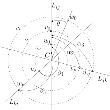
    Figure 13: Concentric polygon of odd number of vertices

  • Now we consider the case when none of the above is true. Let $n_{i}$, $n_{j}$ and $n_{k}$ be the number of vertices of $G_{i}$, $G_{j}$ and $G_{k}$ respectively (Figure 13). $n_{i}$, $n_{j}$ and $n_{k}$ are prime to each other (lemma 20). ${\cal L}_{ij}$ passes through a vertex $u_{0}$ of $G_{i}$ and a vertex $v_{0}$ of $G_{j}$. First we consider the case when both $u_{0}$ and $v_{0}$ lie on the same ray ($R_{ij}$) starting from $C$. Suppose, ${\cal L}_{ij}$ does not pass through any vertex of $G_{k}$. Let $w_{0}$ be the vertex of $G_{k}$ which is closest to ${R}_{ij}$ in the clockwise direction. $Cw_{0}$ makes an angle $\theta$ with $R_{ij}$ at $C$. We label the vertices of $G_{i}$ in the clockwise direction starting from $u_{0}$ and denote them by $u_{1},\ldots,u_{n_{i-1}}$. We label the vertices of $G_{j}$ in the clockwise direction starting from $v_{0}$ and denote them by $v_{1},\ldots,v_{n_{j-1}}$. We label the vertices of $G_{k}$ in the clockwise direction starting from $w_{0}$ and denote them by $w_{1},\ldots,w_{n_{k-1}}$. Suppose, ${\cal L}_{jk}$ passes through the $p^{th}$ vertex $v_{p}$ of $G_{j}$ and the $q^{th}$ vertex $w_{q}$ of $G_{k}$. ${\cal L}_{ki}$ passes through the vertex $w_{r}$ of $G_{k}$ and $u_{s}$ of $G_{i}$. $Cv_{p}$ and $Cw_{q}$ make angles $\alpha_{2}$ and $\alpha_{3}$ respectively with $R_{ij}$. $Cu_{s}$ and $Cw_{r}$ make angles $\beta_{1}$ and $\beta_{3}$ respectively with $R_{ij}$.

    Since, $\alpha_{2}=\alpha_{3}$, we get the following equation:

    $$\frac{p}{n_{j}}=\frac{q}{n_{k}}+\frac{\theta}{360}$$ (4)

    Since, $\beta_{1}=\beta_{3}$,

    $$\frac{s}{n_{i}}=\frac{r}{n_{k}}+\frac{\theta}{360}$$ (5)

    Substituting equation $(4)$ from equation $(5)$,

    $$({\frac{s}{n_{i}}-\frac{p}{n_{j}}}){n_{k}}=r-q$$ (6)

    Since $(r-q)$ is an integer, $({\frac{s}{n_{i}}-\frac{p}{n_{j}}}){n_{k}}$ must be an integer. $0\leq\frac{s}{n_{i}}<1$ and $0\leq\frac{p}{n_{j}}<1$. $|({\frac{s}{n_{i}}-\frac{p}{n_{j}}})|<1$. Since, $n_{i}$, $n_{j}$ and $n_{k}$ are pairwise relatively prime, $({\frac{s}{n_{i}}-\frac{p}{n_{j}}}){n_{k}}=0$. From equation $(4)$, $\frac{s}{n_{i}}=\frac{p}{n_{j}}=\frac{q}{n_{k}}+\frac{\theta}{360}$. Hence, ${\cal L}_{jk}$ is the line of symmetry for $G_{i}$, $G_{j}$ and $G_{k}$.

Figure 14: Concentric polygon of odd number of vertices

Let us consider the case when $u_{0}$ and $v_{0}$ lie at different sides of $C$ (Fig 14). The equations $(4)$ and $(5)$ will now change.

Since, $\alpha_{2}=\alpha_{3}$, we get the following equation:

$$\frac{p}{n_{j}}=\frac{q}{n_{k}}+\frac{\theta}{360}+\frac{180}{360}$$ (7)

Since, $\beta_{1}=\beta_{3}$,

$$\frac{s}{n_{i}}=\frac{r}{n_{k}}+\frac{\theta}{360}$$ (8)

Substituting equation $(7)$ from equation $(8)$,

$$({\frac{s}{n_{i}}-\frac{p}{n_{j}}}+\frac{1}{2}){n_{k}}=r-q$$ (9)

From the argument stated previously, the value of ${\frac{s}{n_{i}}-\frac{p}{n_{j}}}$ is a fraction. If ${\frac{s}{n_{i}}-\frac{p}{n_{j}}}\neq 0$, then it has a fractional part. So, $|({\frac{s}{n_{i}}-\frac{p}{n_{j}}}+\frac{1}{2}){n_{k}})|$ is not a non-zero integer. Since, $r-q$ is an integer, it must be zero. From equation $(7)$, $\frac{s}{n_{i}}=\frac{p}{n_{j}}=\frac{q}{n_{k}}+\frac{\theta}{360}+\frac{1}{2}$. Hence, ${\cal L}_{jk}$ is a common line of symmetry for $G_{i}$, $G_{j}$ and $G_{k}$.

Similarly the result follows for other cases such as when $v_{p}$ and $w_{q}$ lie on different sides of $C$ or $u_{s}$ and $w_{r}$ lie on different sides of $C$.

Theorem 3

Every pair in $\cal G^{\prime}$ is a symmetric pair, if and only if there is a common line of symmetry for all the polygons in $\cal G^{\prime}$.

Proof: If: Trivial.

Only If: We prove this by induction on the number of polygons in $\cal G^{\prime}$. If $\cal G^{\prime}$ contains three polygons then the result follows from lemma 21. Suppose, the statement is true for $p\geq 3$ polygons. Now the ${p+1}^{th}$ polygon say $G_{p+1}$ is introduced. If $G_{p+1}$ has even number of vertices then any line of symmetry for $G_{1\ldots p}$ is a line of symmetry for $G_{p+1}$. Hence the result is true.

Suppose $G_{p+1}$ has odd number of vertices. $<G_{p},G_{(p+1)}>$ is a symmetric pair (given). Since $G_{1},G_{2},\cdots,G_{p}$ has a common line of symmetry (induction hypothesis), that same line is also a common line of symmetry for $<G_{1,2,\cdots,(p-1)},G_{p}>$. Similarly, using the induction hypothesis $<G_{(p+1)},G_{1,2,\cdots,(p-1)}>$ is also a symmetric pair. Hence following lemma 21, $G_{1,2,\cdots,(p-1)}$, $G_{p}$ and $G_{(p+1)}$ have a common line of symmetry, say $\cal L$. Following theorem 2, $\cal L$ is a line of symmetry for $G_{1},\ldots G_{(p-1)}$. Thus the result follows.

Observation 13

If $\cal G$ is symmetric then every pair in $\cal G$ is a symmetric pair.

Theorem 4

$\cal G^{\prime}$ is symmetric if and only if $\cal G$ is symmetric.

Proof: Follows from theorem 2.

Let $P$ be a set of points on the 2D plane. We first identify the SEC for $P$. With respect to the center of the SEC we divide the points of $P$ into a set of concentric polygons ${\cal G}_{P}$.

Theorem 5

$P$ is in $\O_{S}$ iff ${\cal G}_{P}$ is in $\O_{S}$.

Proof:If: If ${\cal G}_{P}$ is in $\O_{S}$, all polygons in $\cal G$ have a common line of symmetry (definition 14). Hence, the vertices in $G_{1}\cup G_{2}\ldots\cup G_{t}$ have a line of symmetry. The set of vertices in $G_{1}\cup G_{2}\ldots\cup G_{t}$, which is $P$, is in $\O_{S}$.

Only If: Let $\cal L$ be a line of symmetry for $P$. $\cal L$ also passes through the center of SEC of $P$ (observation 1). However, $P$ is the set of vertices in $G_{1}\cup G_{2}\ldots\cup G_{t}$. $\cal L$ also is the line of symmetry of the set of vertices in $G_{1}\cup G_{2}\ldots\cup G_{t}$. It is easy to note that the mirror image of any vertex of $G_{i}\in\cal G$, is a vertex of ${\cal G}_{i}$. This implies that, $\cal L$ is the line of symmetry for all $G_{i}\in\cal G$. Therefore all $G_{i}\in\cal G$, are symmetric across $\cal L$. Hence, ${\cal G}_{P}$ is in $\O_{S}$ (definition 14).

Corollary 1

$P$ is in $\O_{A}$ iff ${\cal G}_{P}$ is in $\O_{A}$.

Theorem 6

$P$ is orderable if and only if $P$ is in $\O_{A}$.

Proof: If: If $P$ is in $\O_{A}$, ${\cal G}_{P}$ is in $\O_{A}$ (theorem 5). If ${\cal G}_{P}$ is in $\O_{A}$, there is no common line of symmetry for the polygons in ${\cal G}_{P}$ (definition 14). There exists an asymmetric pair in ${\cal G}_{P}$. Following lemma 15, ${\cal G}_{p}$ is orderable. Hence $P$ is orderable.

Only If: If $P$ is orderable, $P$ is in $\O_{A}$ (lemma 1).

Corollary 2

$P$ is orderable if and only if ${\cal G}_{P}$ is in $\O_{A}$.

5 Algorithms for Leader Election and Gathering of Robots

Let $R$ be a set of robots. From the previous section, we note that if $R$ is orderable, then leader election is possible from $R$. In this case the first robot in the ordering becomes the leader. In this section, we present the leader election algorithm for a set of robots, $R$. $R$ can be viewed as a set of multiple concentric polygons ${\cal G}=G_{1},G_{2},\ldots,G_{t}$ as described previously. The leader election algorithm elects leader from $G_{1}\in{\cal G}$. First we present leader election algorithm for a single polygon $G$. Then we extend the algorithm for the set of concentric polygons $\cal G$.

5.1 Algorithm for checking symmetry in $G$

A polygon may have more than one line of symmetry.

Definition 15

The number of lines of symmetry of $G$ is called the degree of symmetry of $G$.

Algorithms $Check\_Symmetry\_Odd(G)$ and $Check\_Symmetry\_Even(G)$ are used for checking symmetry in $G$ when the numbers of vertices of $G$ are odd and even respectively.

Input: A convex polygon $G$ with $n$ vertices such that $n$ is odd.

Output: Reports the degree of symmetry of $G$ ($0$ if asymmetric)

$deg\_sym=0$;AlgoLine0.1

$i=1$;AlgoLine0.2

while $i\leq n$ do  Compute $CW_{v_{i}}$ and $ACW_{v_{i}}$; AlgoLine0.3

if $CW_{v_{i}}=ACW_{v_{i}}$ then  $deg\_sym=deg\_sym+1$; AlgoLine0.4

else  $i++$ ; AlgoLine0.5

end end if $deg\_sym>0$ then  Report “$G$ is symmetric”; AlgoLine0.6

Report “The degree of symmetry is:” $deg\_sym$;AlgoLine0.7

else  Report “$G$ is asymmetric”; AlgoLine0.8

end

Algorithm 1 $Check\_Symmetry\_Odd(G)$

8

8

8

8

8

8

8

8

Correctness of Check_Symmetry_Odd(G): Follows from theorem 1.

Input: A convex polygon $G$ with $n$ vertices such that $n$ is even

Output: Reports the degree of symmetry of $G$ ($0$ if asymmetric)

AlgoLine0.1

$deg\_sym=0$;AlgoLine0.2

$i=1$;AlgoLine0.3

$st\_sym=False$;AlgoLine0.4

$sk\_sym=False$;AlgoLine0.5

AlgoLine0.6

while $i\leq n$ do  Compute $CW_{v_{i}}$ and $ACW_{v_{i}}$; AlgoLine0.7

if $CW_{v_{i}}=ACW_{v_{i}}$ then  $st\_sym=True$; AlgoLine0.8

$deg\_sym=deg\_sym+1$;AlgoLine0.9

else  for j = 1 to i-1 do  if ($CW_{v_{i}}=CW_{v_{j}}$) $\vee$ ($CW_{v_{i}}=ACW_{v_{j}}$) $\vee$ ($ACW_{v_{i}}=CW_{v_{j}}$) then  $sk\_sym=True$; AlgoLine0.10

$deg\_sym=deg\_sym+1$;AlgoLine0.11

end end $i++$;AlgoLine0.12

end end if $deg\_sym>0$ $\wedge$ $st\_sym=True$ then  Report “$G$ is straight symmetric”; AlgoLine0.13

Report “The degree of symmetry is:” $deg\_sym/2$;AlgoLine0.14

end if $deg\_sym>0$ $\wedge$ $sk\_sym=True$ then  Report “$G$ is skew symmetric”; AlgoLine0.15

Report “The degree of symmetry is:” $deg\_sym/2$;AlgoLine0.16

end if $deg\_sym=0$ then  Report “$G$ is asymmetric”; AlgoLine0.17

end

Algorithm 2 $Check\_Symmetry\_Even(G)$

17

17

17

17

17

17

17

17

17

17

17

17

17

17

17

17

17

Correctness of Check_Symmetry_Even(G): Follows from theorem 1.

Note that if $G$ has even number of vertices then every line of symmetry (straight or skewed) passes through 2 vertices and is counted twice. Therefore, the algorithm returns the $deg\_sum$ by dividing it by $2$.

Next we present a leader election algorithm, when the convex polygon has degree of symmetry one.

Input: A symmetric convex polygon $G$ of $n$ vertices.

Output: A vertex $v_{l}$ or reports that leader election is not possible.

if $n$ is odd then  Call $Check\_Symmetry\_Odd(G)$; AlgoLine0.1

if degree of symmetry of $G>1$ then  Report “Leader Election is not possible for $G$”; AlgoLine0.2

end if degree of symmetry of $G$ = $1$ then  $v_{l}$ = $v_{i}\in G$ such that $CW(v_{i})=ACW(v_{i})$; AlgoLine0.3

Return $v_{l}$;AlgoLine0.4

end else  Call $Chekc\_Symmetry\_Even(G)$; AlgoLine0.5

if degree of symmetry of $G>1$ then  Report “Leader Election is not possible for $G$”; AlgoLine0.6

end if degree of symmetry of $G$ = $1$ and the line of symmetry passes through either a single vertex or through two vertices. then  Find two vertices $v_{i}$ and $v_{j}$ such that $CW(v_{i})=ACW(v_{i})$ and $CW(v_{j})=ACW(v_{j})$; AlgoLine0.7

$VI=CW(v_{i})$;AlgoLine0.8

$VJ=CW(v_{j})$;AlgoLine0.9

if $VI>VJ$ then  return $v_{i}$ as leader; AlgoLine0.10

else  return $v_{j}$ as leader; AlgoLine0.11

end else  Report “Leader Election is not possible for $G$”; AlgoLine0.12

end end

Algorithm 3 $Elect\_Leader\_Sym(G)$

12

12

12

12

12

12

12

12

12

12

12

12

Correctness of Elect_Leader_Sym(G): Follows from theorem 1.

Observation 14

If the degree of symmetry of a convex symmetric polygon is one and the line of symmetry passes through two vertices of the polygon, then leader election is possible.

Once the leader is elected for a symmetric polygon with degree of symmetry one, the leader can be moved such a way that the new polygon becomes asymmetric. Following algorithm does this task.

Input: A convex polygon $G$ with degree of symmetry one. The line of symmetry passes through either a single vertex or through two vertices.

Output: An asymmetric polygon convex $G$.

$v_{l}$ = $Elect\_Leader\_Sym(G)$;AlgoLine0.1

Move $v_{l}$, $\epsilon$ distance, to its right side, on the circumference of the circle inscribing $G$;AlgoLine0.2

return $G$;AlgoLine0.3

Algorithm 4 $Make\_SymToAsym(G)$

3

3

3

Correctness of Make_SymToAsym(G): Whenever the leader $v_{l}$ moves from its position, $G$ becomes asymmetric. Then no other robot executes the algorithm $Make\_SymToAsym(G)$. Therefore, there is no chance that $G$ becomes symmetric again.

Following algorithm elects leader when $G$ is asymmetric.

Input: An asymmetric convex polygon $G$ with $n$ vertices.

Output: A leader vertex $v_{l}$. The new positions of $G\setminus v_{l}$ are asymmetric.

for k =1 to n do  Compute the tuple $\{CW(v_{k}),ACW(v_{k})\}$; AlgoLine0.1

end $\{CW(v_{m}),ACW(v_{m})\}$ = lexicographic minimum of $\{(CW(v_{1}),ACW(v_{1})),\ldots,(CW(v_{n}),ACW(v_{n}))\}$;AlgoLine0.2

if $CW(v_{m})<ACW(v_{m})$ then  $CW(v_{m})$ is the ordering of $G$; AlgoLine0.3

else  $ACW(v_{m})$ is the ordering of $G$;AlgoLine0.4