Inverse scattering at a fixed energy for Discrete Schrödinger Operators on the square lattice

Abstract.

We study an inverse scattering problem for the discrete Schrödinger operator on the square lattice ${\bf Z}^{d}$, $d\geq 2$, with compactly supported potential. We show that the potential is uniquely reconstructed from a scattering matrix for a fixed energy.

1. Introduction

1.1. Inverse scattering

Let ${\bf Z}^{d}=\{n=(n_{1},\cdots,n_{d})\,;\,n_{i}\in{\bf Z},\ 1\leq i\leq d\}$ be the square lattice, and $e_{1}=(1,0,\cdots,0),\cdots,e_{d}=(0,\cdots,0,1)$ the standard basis of ${\bf Z}^{d}$. Throughout the paper, we shall assume that $d\geq 2$. The Schrödinger operator ${\widehat{H}}$ on ${\bf Z}^{d}$ is defined by

$${\widehat{H}}={\widehat{H}}_{0}+{\widehat{V}},$$

where for ${\widehat{f}}=\{\widehat{f}(n)\}_{n\in{\bf Z}^{d}}\in\ell^{2}({\bf Z}^{d})$ and $n\in{\bf Z}^{d}$

$$\big{(}{\widehat{H}}_{0}\widehat{f}\big{)}(n)=-\frac{1}{4}\sum_{j=1}^{d}\big{\{}{\widehat{f}}(n+e_{j})+{\widehat{f}}(n-e_{j})\big{\}}+\frac{d}{2}\widehat{f}(n),$$

$$({\widehat{V}}{\widehat{f}})(n)=\widehat{V}(n){\widehat{f}}(n).$$

We impose the following assumption on $\widehat{V}$:

(A) $\ \widehat{V}$ is real-valued, and $\widehat{V}(n)=0$ except for a finite number of $n$.

Under this assumption, $\sigma(\widehat{H}_{0})=\sigma_{ess}(\widehat{H})=[0,d]$, and the wave operators

(1.1) $$\widehat{W}^{(\pm)}={\mathop{\rm s-lim}_{t\to\pm\infty}}\,e^{it\widehat{H}}e^{-it\widehat{H}_{0}}\quad({\rm in}\ \ell^{2}({\bf Z}^{d}))$$

exist and are asymptotically complete, i.e. their ranges coincide with ${\mathcal{H}}_{ac}(\widehat{H})$, the absolutely continuous subspace for $\widehat{H}$. Hence the scattering operator

(1.2) $$\widehat{S}=\big{(}\widehat{W}^{(+)}\big{)}^{\ast}\widehat{W}^{(-)}$$

is unitary. Associated with $\widehat{H}_{0}$, we have a unitary spectral representation

$$\widehat{\mathcal{F}}_{0}:\ell^{2}({\bf Z}^{d})\to L^{2}((0,d);L^{2}(M_{\lambda});d\lambda),$$

where

(1.3) $$M_{\lambda}=\Big{\{}x\in{\bf T}^{d}\,;\,d-\sum_{j=1}^{d}\cos x_{j}=2\lambda\Big{\}},$$

(1.4) $${\bf T}^{d}={\bf R}^{d}/(2\pi{\bf Z})^{d}=[-\pi,\pi]^{d}.$$

Then $\widehat{\mathcal{F}}_{0}\widehat{S}(\widehat{\mathcal{F}}_{0})^{\ast}$ has the following direct integral representation

(1.5) $$\widehat{\mathcal{F}}_{0}\widehat{S}(\widehat{\mathcal{F}}_{0})^{\ast}=\int_{0}^{d}\oplus\,\mathcal{S}(\lambda)\,d\lambda.$$

Here $\mathcal{S}(\lambda)$ is a unitary operator on $L^{2}(M_{\lambda})$, and is called the S-matrix.

Our main concern in this paper is the inverse scattering, i.e. reconstruction of the potential $\widehat{V}$ from the knowledge of the S-matrix. In [10] (see also [6]), it has been proven that given $\mathcal{S}(\lambda)$ for all energy $\lambda\in(0,d)\setminus{\bf Z}$, one can uniquely reconstruct the potential.

It is worthwhile to recall the case of the continuous model, i.e. the Schrödinger operator $-\Delta+V(x)$ in $L^{2}({\bf R}^{d})$. In this case, it is known that only one arbitrarily fixed energy $\lambda>0$ is sufficient to reconstruct the compactly supported (and also exponentially decaying) potential $V(x)$ from the S-matrix $\mathcal{S}(\lambda)$. This was proved for $d\geq 3$ in 1980’s by Sylvester-Uhlmann [20], Nachman [15], Khenkin-Novikov [12]. There are two methods. One way is applicable to the compactly supported potential and based on the equivalence of the S-matrix and the Dirichlet-Neumann map (called D-N map hereafter) for the boundary value problem in a bounded domain. The other way relies on Faddeev’s theory for the multi-dimensional inverse scattering, in particular, on Feddeev’s scattering amplitude, and allows exponentially decaying potentials. In both cases, Sylvester-Uhlmann’s complex geometrical optics solutions to the Schrödinger equation, or Faddeev’s exponentially growing Green function played a crucial role. (See e.g. an expositiory article [9].) However, since both of these methods use the complex Born approximation, the case $d=2$ remained open rather long time. Note that for the potential of the form coming from ellectric conductivities, the 2-dim. inverse scattering problem for a fixed energy was solved by Nachman [16]. See also [8]. Recently Bukhgeim [2] proved that, based on Carleman estimates, the D-N map determines the potential for the 2-dim. boundary value problem. For the partial data problem, see [7]. This result can be applied to the inverse scattering and to derive an affirmative answer to the uniqueness of the potential for given potential of fixed energy.

1.2. Main result

To study the inverse scattering from a fixed energy for the discrete model, we adopt the above-mentioned former approach. Namely, we assume that the potential is compactly supported, and derive the equivalence of the S-matrix and the D-N map in a bounded domain.

We need to restrcit the energy in some interval. Let

(1.6) $$I_{d}=\left\{\begin{array}[]{lc}(0,1)\cup(0,1),&{\rm for}\quad d=2,\\ (0,1/2)\cup(d-1/2,d),&{\rm for}\quad d\geq 3.\end{array}\right.$$

The following theorem is our main aim.

Theorem 1.1.

Fix $\lambda\in I_{d}$ arbitrarily. Then from the S-matrix $\mathcal{S}(\lambda)$, one can uniquely reconstruct the potential $\widehat{V}$.

Our proof not only states the uniqueness, but also explains the procedure of the reconstuction of the potential.

1.3. The plan of the proof

After the preparation of basic spectral results in §2 and §3, the first task is to relate the S-matrix with the far-field pattern at infinity of the generalized eigenfunction of $\widehat{H}$. This is done in §4 by observing the asymptotic expansion at infinity of the Green operator of $\widehat{H}$. In §5, we introduce the radiation condition for the Helmholtz equation and prove the uniqueness theorem for the solution. We then study the spectral theory for the exterior problem in §6, with the aid of which we obtain in §7 the equivalence of the S-matrix and the D-N map for a boundary value problem in a bounded domain. The potential is then reconstructed from the D-N map in §8 via a constructive procedure.

Although the main stream of the proof is the same as the continuous case, we need to be careful about the difference in the case of the discrete model. The first one is the asymptotic expansion of the resolvent at infinity. This is based on the stationary phase method on the surface $M_{\lambda}$ defined by (1.3), which is not strictly convex in general. This is the reason we restrict the energy on $I_{d}$. The second one, which is more serious, occurs when we compare the far-field patterns of solutions to Schrödinger equations in the whole space with those of the exterior domain. We need a Rellich type theorem (see Theorem 5.7) and a unique continuation property for the discrete Helmholtz equation, which do not seem to be well-known. However, the former’s precursor has been given by Shaban-Vainberg [19], and the latter follows rather easily from it. As a byproduct, it proves the non-existence of embedded eigenvalues for $\widehat{H}$ ([11]). We then go into the final step of computing the potential from the D-N map. In the continuous case, this is an elliptic Cauchy problem from the boundary, hence is ill-posed. However, in the discrete case, this is a finite dimensional problem, therefore a finite computational procedure. The whole proof does not depend on the space dimension. In contrust, it took a long time to get the 2-dim. result in the continuous case.

1.4. Remarks for references

There are important precursors of this paper. The work of Eskina [6] have already announced the result of the inverse scattering for discrete Schrödinger operators. In particular, this paper stresses the effectiveness of several complex variables in the study of discrete Schrödinger operators. Shaban-Vainberg [19] studied the spectral theory of discrete Schrödinger operators. They introduced the radiation condition, proved the limiting absorption principle, and derived the asymptotic expansion of the resolvent at infinity including the case of non-convex surface.

The computation of the D-N map for the discrete interior boundary value problem was done in the work of Oberlin [17]. See also Curtis-Morrow [3] and Curtis-Mooers-Morrow [4].

1.5. Notation

$C$’s denote various constants. For any $x,y\in{\bf R}^{d}$, $x\cdot y=x_{1}y_{1}+\cdots+x_{d}y_{d}$ denotes the ordinary scalar product in the Euclidean space where $x_{j}$ and $y_{j}$ are $j$-th component of $x$ and $y$ respectively. For any $x\in{\bf R}^{d}$, $|x|=(x\cdot x)^{1/2}$ is the Euclidean norm. Note that even for $n=(n_{1},\cdots,n_{d})\in{\bf Z}^{d}$, we use $|n|=\big{(}\sum_{j=1}^{d}|n_{j}|^{2}\big{)}^{1/2}$. For two Banach spaces $X$ and $Y$, $\mathbf{B}(X,Y)$ denotes the totality of bounded operators from $X$ to $Y$. For a self-adjoint operator $A$ on a Hilbert space, $\sigma(A)$, $\sigma_{ess}(A)$, $\sigma_{disc}(A)$, $\sigma_{ac}(A)$ and $\sigma_{p}(A)$ denote its spectrum, essential spectrum, discrete spectrum, absolutely continuous spectrum and point spectrum, respectively. For a set $S$, $\,{}^{\#}S$ denotes the number of elements in $S$. We use the notation

$$\langle t\rangle=(1+t^{2})^{1/2},\quad t\in{\bf R}.$$

1.6. Acknowledgement

The authors are indebted to Evgeny Korotyaev for useful discussions and encouragements. The second author is supported by the Japan Society for the Promotion of Science under the Grant-in-Aid for Research Fellow (DC2) No. 23110.

2. Momentum representation

2.1. Discrete Fourier transform

From the view point of dynamics on the lattice, the torus ${\bf T}^{d}$ in (1.4) plays the role of momentum space. Let ${\mathcal{U}}$ be the unitary operator from $\ell^{2}({\bf Z}^{d})$ to $L^{2}({\bf T}^{d})$ defined by

$$({\mathcal{U}}\,{\widehat{f}})(x)=(2\pi)^{-d/2}\sum_{n\in{\bf Z}^{d}}{\widehat{f}}(n)e^{-in\cdot x}.$$

Using this discrete Fourier transformation, the Hamiltonian $\widehat{H}$ is represented by

$$H={\mathcal{U}}\,{\widehat{H}}\,{\mathcal{U}}^{\ast}=H_{0}+V,\quad H_{0}={\mathcal{U}}\,{\widehat{H}_{0}}\,{\mathcal{U}}^{\ast},\quad V={\mathcal{U}}\,{\widehat{V}}\,{\mathcal{U}}^{\ast},$$

where $H_{0}$ is the multiplcation operator:

(2.1) $$H_{0}=\frac{1}{2}\Big{(}d-\sum_{j=1}^{d}\cos x_{j}\Big{)}=:h(x),$$

and $V$ is the convolution operator

$$(Vu)(x)=(2\pi)^{-d/2}\int_{{\bf T}^{d}}V(x-y)u(y)dy,\quad V(x)=(2\pi)^{-d/2}\sum_{n\in{\bf Z}^{d}}\widehat{V}(n)e^{-in\cdot x}.$$

2.2. Sobolev and Besov spaces

We define operators $\widehat{N}_{j}$ and $N_{j}$ by

$$\big{(}\widehat{N}_{j}\widehat{f})(n)=n_{j}\widehat{f}(n),\quad N_{j}=\mathcal{U}\widehat{N}_{j}\mathcal{U}^{\ast}=i\frac{\partial}{\partial x_{j}}.$$

We put $N=(N_{1},\cdots,N_{d})$, and let $N^{2}$ be the self-adjont operator defined by

$$N^{2}=\sum_{j=1}^{d}N_{j}^{2}=-\Delta,\quad{\rm on}\quad{\bf T}^{d},$$

where $\Delta$ denotes the Laplacian on ${\bf T}^{d}=[-\pi,\pi]^{d}$ with periodic boundary condition. We put

$$|N|=\sqrt{N^{2}}=\sqrt{-\Delta}.$$

For $s\in{\bf R}$, let ${\mathcal{H}}^{s}$ be the completion of $D(|N|^{s})$ with respect to the norm $\|u\|_{s}=\|\langle N\rangle^{s}u\|$ :

$${\mathcal{H}}^{s}=\{u\in{\mathcal{D}}^{\prime}({\bf T}^{d})\,;\,\|u\|_{s}=\|\langle N\rangle^{s}u\|<\infty\},$$

where $\mathcal{D}^{\prime}({\bf T}^{d})$ denotes the space of distribution on ${\bf T}^{d}$. Put $\mathcal{H}=\mathcal{H}^{0}=L^{2}({\bf T}^{d})$.

For a self-adjoint operator $T$, let $\chi(a\leq T<b)$ denote the operator $\chi_{I}(T)$, where $\chi_{I}(\lambda)$ is the characteristic function of the interval $I=[a,b)$. The operators $\chi(T<a)$ and $\chi(T\geq b)$ are defined similarly. Using the series $\{r_{j}\}_{j=0}^{\infty}$ with $r_{-1}=0$, $r_{j}=2^{j}\ (j\geq 0)$, we define the Besov space $\mathcal{B}$ by

$$\mathcal{B}=\Big{\{}f\in{\mathcal{H}}\,;\|f\|_{\mathcal{B}}=\sum_{j=0}^{\infty}r_{j}^{1/2}\|\chi(r_{j-1}\leq|N|<r_{j})f\|<\infty\Big{\}}.$$

Its dual space $\mathcal{B}^{\ast}$ is the completion of $\mathcal{H}$ by the following norm

$$\|u\|_{\mathcal{B}^{\ast}}=\sup_{j\geq 0}r_{j}^{-1/2}\|\chi(r_{j-1}\leq|N|<r_{j})u\|.$$

The following Lemma 2.1 is proved in the same way as in [1].

Lemma 2.1.

(1) There exists a constant $C>0$ such that

$$C^{-1}\|u\|_{\mathcal{B}^{\ast}}\leq\left(\sup_{R>1}\frac{1}{R}\|\chi(|N|<R)u\|^{2}\right)^{1/2}\leq C\|u\|_{\mathcal{B}^{\ast}}.$$

Therefore, in the following, we use

$$\|u\|_{\mathcal{B}^{\ast}}=\left(\sup_{R>1}\frac{1}{R}\|\chi(|N|<R)u\|^{2}\right)^{1/2}$$

as a norm on $\mathcal{B}^{\ast}$.
(2) For $s>1/2$, the following inclusion relations hold :

$$\mathcal{H}^{s}\subset\mathcal{B}\subset\mathcal{H}^{1/2}\subset\mathcal{H}\subset\mathcal{H}^{-1/2}\subset\mathcal{B}^{\ast}\subset\mathcal{H}^{-s}.$$

We also put $\widehat{\mathcal{H}}=\ell^{2}({\bf Z}^{d})$, and define $\widehat{\mathcal{H}}^{s}$, $\widehat{\mathcal{B}}$, $\widehat{\mathcal{B}}^{\ast}$ by replacing $N$ by $\widehat{N}$. Note that $\widehat{\mathcal{H}}^{s}=\mathcal{U}^{\ast}\mathcal{H}^{s}$ and so on. In particular, Parseval’s formula implies that

$$\|u\|_{\mathcal{H}^{s}}^{2}=\|\widehat{u}\|_{\widehat{\mathcal{H}}^{s}}^{2}=\sum_{n\in{\bf Z}^{d}}(1+|n|^{2})^{s}|\widehat{u}(n)|^{2},$$

$$\|u\|_{{\mathcal{B}}^{\ast}}^{2}=\|\widehat{u}\|_{\widehat{\mathcal{B}}^{\ast}}^{2}=\sup_{R>1}\frac{1}{R}\sum_{|n|<R}|\widehat{u}(n)|^{2},$$

$\widehat{u}(n)$ being the Fourier coefficient of $u(x)$.

2.3. Resolvent estimate

Lemma 2.2.

(1) $\ \sigma(\widehat{H}_{0})=\sigma_{ac}(\widehat{H}_{0})=[0,d]$.
(2)    $\sigma_{ess}(\widehat{H})=[0,d],\quad\sigma_{disc}(\widehat{H})\subset{\bf R}\setminus[0,d]$.
(3)    $\sigma_{p}(\widehat{H})\cap\big{(}(0,d)\setminus{\bf Z}\big{)}=\emptyset$.

Proof. The assertions (1), (2) follow from (2.1) and Weyl’s theorem. The assertion (3) is proven in [11]. ∎

Let $\widehat{R}(z)=(\widehat{H}-z)^{-1}$.

Theorem 2.3.

(1) Let $s>1/2$ and $\lambda\in(0,d)\setminus{\bf Z}$. Then there exists a norm limit $\widehat{R}(\lambda\pm i0):=\lim_{\epsilon\to 0}\widehat{R}(\lambda\pm i\epsilon)\in{\bf B}(\widehat{\mathcal{H}}^{s};\widehat{\mathcal{H}}^{-s})$. Moreover, we have

(2.2) $$\sup_{\lambda\in J}\|\widehat{R}(\lambda\pm i0)\|_{{\bf B}(\widehat{\mathcal{B}};\widehat{\mathcal{B}}^{\ast})}<\infty.$$

for any compact interval $J$ in $(0,d)\setminus{\bf Z}$. The mapping $(0,d)\setminus{\bf Z}\ni\lambda\mapsto\widehat{R}(\lambda\pm i0)$ is norm continuous in ${\bf B}(\widehat{\mathcal{H}}^{s};\widehat{\mathcal{H}}^{-s})$ and weakly continuous in ${\bf B}(\widehat{\mathcal{B}}\,;\widehat{\mathcal{B}}^{\ast})$.
(2) $\widehat{H}$ has no singular continuous spectrum.

For the proof of Theorem 2.2, see Lemma 2.5 and Theorem 2.6 of [10]. Note that

(2.3) $$\nabla h(x)=0\Longleftrightarrow h(x)\in\{0,1,\cdots,d\}.$$

This is the reason why the set of thresholds $\{0,1,\cdots,d\}$ appears.

3. Spectral representations and S-matrices

We recall spectral representations and S-matrices derived in §3 of [10].

3.1. Spectral representation on the torus

We begin with the spectral representation in the momentum space. Let us note

$$h(x)=\frac{1}{2}\Big{(}d-\sum_{j=1}^{d}\cos x_{j}\Big{)}=\sum_{j=1}^{d}\sin^{2}\left(\frac{x_{j}}{2}\right),$$

which suggests that the variables $y=(y_{1},\cdots,y_{d})\in[-1,1]^{d}$:

$$y_{j}=\sin\frac{x_{j}}{2},\quad x_{j}=2\arcsin y_{j}$$

are convenient to describe $H_{0}$. Note that for $\lambda\in(0,d)\setminus{\bf Z}$

(3.1) $$x(\sqrt{\lambda}\theta)=\left(2\arcsin(\sqrt{\lambda}\theta_{1}),\cdots,2\arcsin(\sqrt{\lambda}\theta_{d})\right),\quad\theta\in S^{d-1},$$

gives a parametric representation of

(3.2) $$M_{\lambda}=\big{\{}x\in{\bf T}^{d}\,;\,h(x)=\lambda\big{\}}.$$

We equip $M_{\lambda}$ with the measure

$$d\widetilde{M}_{\lambda}=\frac{(\sqrt{\lambda})^{d-2}}{2}J(\sqrt{\lambda}\theta)d\theta,$$

$$J(y)=\chi(y){\mathop{\prod}_{j=1}^{d}}\,\frac{2}{\cos(x_{j}/2)}=\chi(y){\mathop{\prod}_{j=1}^{d}}\,\frac{2}{\sqrt{1-y_{j}^{2}}},$$

$\chi(y)$ being the characteristic function of $[-1,1]^{d}$. Then we have

$$dx=J(y)dy=\,d\widetilde{M}_{\lambda}d\lambda,\quad d\widetilde{M}_{\lambda}=\frac{dM_{\lambda}}{|\nabla_{x}h(x)|},$$

where $dM_{\lambda}$ is the measure on $M_{\lambda}$ induced from $dx$. Let $L^{2}(M_{\lambda})$ be the Hilbert space with inner product

$$(\varphi,\psi)_{L^{2}(M_{\lambda})}=\int_{M_{\lambda}}\varphi\,\overline{\psi}\,d\widetilde{M}_{\lambda}.$$

We define $\mathcal{F}_{0}(\lambda)f={\rm Tr}_{M_{\lambda}}f$, where ${\rm Tr}_{M_{\lambda}}$ is the trace on $M_{\lambda}$. More precisely,

(3.3) $$\left(\mathcal{F}_{0}(\lambda)f\right)(\theta)=f(x(\sqrt{\lambda}\theta)).$$

It then follows for $R_{0}(z)=(H_{0}-z)^{-1}$

$$\frac{1}{2\pi i}((R_{0}(\lambda+i0)-R_{0}(\lambda-i0))f,g)_{L^{2}({\bf T}^{d})}=(\mathcal{F}_{0}(\lambda)f,\mathcal{F}_{0}(\lambda)g)_{L^{2}(M_{\lambda})},$$

for $\lambda\in(0,d)\setminus{\bf Z}$ and $f,g\in C^{1}({\bf T}^{d})$. We then have by (2.2)

(3.4) $$\mathcal{F}_{0}(\lambda)\in{\bf B}(\mathcal{B};L^{2}(M_{\lambda})).$$

Using this formula, we can derive the spectral representations of $H_{0}$ and $H$. However, we omit it.

3.2. Spectral representation on the lattice

We define the distribution $\delta(h(x)-\lambda)\in\mathcal{D}^{\prime}({\bf T}^{d})$ by

$$\int_{{\bf T}^{d}}f(x)\delta(h(x)-\lambda)dx:=\int_{M_{\lambda}}f(x)\,d\widetilde{M}_{\lambda},\quad f\in C^{\infty}({\bf T}^{d}).$$

Then, from the definition of $\mathcal{F}_{0}(\lambda)^{\ast}$:

$$\big{(}\mathcal{F}_{0}(\lambda)f,\,\phi\big{)}_{L^{2}(M_{\lambda})}=\big{(}f,\,\mathcal{F}_{0}(\lambda)^{\ast}\phi\big{)}_{L^{2}({\bf T}^{d})},$$

we see that $\mathcal{F}_{0}(\lambda)^{\ast}$ defines a distribution on ${\bf T}^{d}$ by the following formula

$$\mathcal{F}_{0}(\lambda)^{\ast}\phi=\phi(x)\delta(h(x)-\lambda).$$

Here the right-hand side makes sense when, for example, $\phi\in C^{\infty}(M_{\lambda})$ and is extended to a $C^{\infty}$-function near $M_{\lambda}$. Then $\widehat{\mathcal{F}}_{0}(\lambda)^{\ast}\phi=\mathcal{U}^{\ast}\mathcal{F}_{0}(\lambda)^{\ast}\phi$ is computed as

(3.5) $$\begin{split}&(2\pi)^{-d/2}\int_{{\bf T}^{d}}e^{in\cdot x}\phi(x)\delta(h(x)-\lambda)dx\\ =&(2\pi)^{-d/2}\int_{M_{\lambda}}e^{in\cdot x}\phi(x)\,d\widetilde{M}_{\lambda}\\ =&(2\pi)^{-d/2}\int_{S^{d-1}}e^{in\cdot x(\sqrt{\lambda}\theta)}\phi(x(\sqrt{\lambda}\theta))\,\frac{(\sqrt{\lambda})^{d-2}}{2}J(\sqrt{\lambda}\theta)\,d\theta.\end{split}$$

In the lattice space, we define $\widehat{\psi}^{(0)}(\lambda,\theta)=\big{\{}\widehat{\psi}^{(0)}(n,\lambda,\theta)\big{\}}_{n\in{\bf Z}^{d}}$, where

(3.6) $$\begin{split}\widehat{\psi}^{(0)}(n,\lambda,\theta)&=(2\pi)^{-d/2}\frac{(\sqrt{\lambda})^{d-2}}{2}e^{in\cdot x(\sqrt{\lambda}\theta)}J(\sqrt{\lambda}\theta)\\ &=(2\pi)^{-d/2}2^{d-1}(\sqrt{\lambda})^{d-2}\chi(\sqrt{\lambda}\theta)\frac{e^{in\cdot x(\sqrt{\lambda}\theta)}}{{\mathop{\prod}_{j=1}^{d}}\cos\big{(}x_{j}(\sqrt{\lambda}\theta)/2\big{)}}.\end{split}$$

Here $\chi(y)$ is the characteristic function of $[-1,1]^{d}$, and $x(\sqrt{\lambda}\theta)$ is defined by (3.1). By (3.5) and (3.6), we have for $\phi\in L^{2}(M_{\lambda})$

$$\begin{split}(\widehat{\mathcal{F}}_{0}(\lambda)^{\ast}\phi)(n)&=(2\pi)^{-d/2}\int_{M_{\lambda}}e^{in\cdot x}\phi(x)\,d\widetilde{M}_{\lambda}\\ &=\int_{S^{d-1}}{\widehat{\psi}}^{(0)}(n,\lambda,\theta)\phi(x(\sqrt{\lambda}\theta))\,d\theta.\end{split}$$

We can also see for rapidly decreasing $\widehat{f}$ on ${\bf Z}^{d}$

$$(\widehat{\mathcal{F}}_{0}(\lambda)\widehat{f})(x(\sqrt{\lambda}\theta))=(2\pi)^{-d/2}\sum_{n\in{\bf Z}^{d}}e^{-in\cdot x(\sqrt{\lambda}\theta)}\widehat{f}(n).$$

The spectral representation for $\widehat{H}$ is constructed as follows. We put

(3.7) $$\widehat{\mathcal{F}}^{(\pm)}(\lambda)=\widehat{\mathcal{F}}_{0}(\lambda)\left(1-\widehat{V}\widehat{R}(\lambda\pm i0)\right),\quad\lambda\in(0,d)\setminus{\bf Z}.$$

Then by (3.4) and (2.2)

$$\widehat{\mathcal{F}}^{(\pm)}(\lambda)\in{\bf B}(\widehat{\mathcal{B}}\,;L^{2}(M_{\lambda})).$$

We define the operator $\widehat{\mathcal{F}}^{(\pm)}$ by $\big{(}\widehat{\mathcal{F}}^{(\pm)}f\big{)}(\lambda)=\widehat{\mathcal{F}}^{(\pm)}(\lambda)f$ for $f\in\widehat{\mathcal{B}}$.

Theorem 3.1.

(1) $\widehat{\mathcal{F}}^{(\pm)}$ is uniquely extended to a partial isometry with initial set $\mathcal{H}_{ac}(\widehat{H})$ and final set $L^{2}({\bf T}^{d})$. Moreover it diagonalizes $\widehat{H}$:

(3.8) $$\big{(}\widehat{\mathcal{F}}^{(\pm)}\widehat{H}\widehat{f}\big{)}(\lambda)=\lambda\big{(}\widehat{\mathcal{F}}^{(\pm)}\widehat{f}\big{)}(\lambda),\quad\widehat{f}\in\mathcal{H}_{ac}(\widehat{H}).$$

(2) The following inversion formula holds:

(3.9) $$\widehat{f}=\mathop{\rm s-lim}_{N\to\infty}\int_{I_{N}}\widehat{\mathcal{F}}^{(\pm)}(\lambda)^{\ast}\big{(}\widehat{\mathcal{F}}^{(\pm)}\widehat{f}\big{)}(\lambda)d\lambda,\quad\widehat{f}\in\mathcal{H}_{ac}(\widehat{H}),$$

where $I_{N}$ is a union of compact intervals in $(0,d)\setminus{\bf Z}$ such that $I_{N}\to(0,d)\setminus{\bf Z}$.
(3) $\widehat{\mathcal{F}}^{(\pm)}(\lambda)^{\ast}\in{\bf B}(L^{2}(M_{\lambda})\,;\,\widehat{\mathcal{B}}^{\ast})$ is an eigenoperator for $\widehat{H}$ in the sense that

$$(\widehat{H}-\lambda)\widehat{\mathcal{F}}^{(\pm)}(\lambda)^{\ast}\phi=0,\quad\phi\in L^{2}(M_{\lambda}).$$

(4) The wave operators

$$\widehat{W}^{(\pm)}={\mathop{\rm s-lim}_{t\to\pm\infty}}\,e^{it\widehat{H}}e^{-it\widehat{H}_{0}}$$

exist and are complete. Moreover,

$${\widehat{W}}^{(\pm)}=\big{(}\widehat{\mathcal{F}}^{(\pm)}\big{)}^{\ast}\widehat{\mathcal{F}}_{0}.$$

3.3. Scattering matrix

The scattering operator $\widehat{S}$ is defined by

$$\widehat{S}=\big{(}\widehat{W}_{+}\big{)}^{\ast}\widehat{W}_{-}.$$

We conjugate it by the spectral representation. Let

$$\mathcal{S}=\widehat{\mathcal{F}}_{0}\widehat{S}(\widehat{\mathcal{F}}_{0})^{\ast},$$

which is unitary on $L^{2}((0,d);L^{2}(M_{\lambda});d\lambda)$. Since $\mathcal{S}$ commutes with $\widehat{H}_{0}$, ${\mathcal{S}}$ is written as a direct integral

$${\mathcal{S}}=\int_{(0,d)}{\oplus}{\mathcal{S}}(\lambda)d\lambda.$$

The S-matrix, ${\mathcal{S}}(\lambda)$, is unitary on $L^{2}(M_{\lambda})$ and has the following representation.

Theorem 3.2.

Let $\lambda\in(0,d)\setminus{\bf Z}$. Then ${\mathcal{S}}(\lambda)$ is written as

$${\mathcal{S}}(\lambda)=1-2\pi iA(\lambda),$$

where

(3.10) $$A(\lambda)=\widehat{\mathcal{F}}_{0}(\lambda)\left(1-\widehat{V}\widehat{R}(\lambda+i0)\right)\widehat{V}\widehat{\mathcal{F}}_{0}(\lambda)^{\ast}=\widehat{\mathcal{F}}^{(+)}(\lambda)\widehat{V}\widehat{\mathcal{F}}_{0}(\lambda)^{\ast},$$

and is called the scattering amplitude.

4. Asymptotic expansion of the resolvent at infinity

4.1. Stationary phase method on a surface

Let $S$ be a compact $C^{\infty}$-surface in ${\bf R}^{d}$ of codimension 1, and $dS$ the measure on $S$ induced from the Euclidean metric. For $a(x)\in C^{\infty}(S)$ and $k\in{\bf R}^{d}$, we put

(4.1) $$I(k)=\int_{S}e^{ix\cdot k}a(x)dS.$$

Theorem 4.1.

Let $N(x)$ be an outward unit normal field on $S$, and $W(x)$, $K(x)$ the Weingarten map and the Gaussian curvature at $x\in S$, respectively. Assume that there exists a finite number of points $x^{(j)}_{\pm}\in S$, $j=1,\cdots,{\nu}$, such that

$$k/|k|=\pm N(x_{\pm}^{(j)}),$$

and that $K(x_{\pm}^{(j)})\neq 0$, $j=1,\cdots,\nu$. Then we have as $\rho=|k|\to\infty$

(4.2) $$\begin{split}I(k)&=\rho^{-(d-1)/2}\sum_{j=1}^{\nu}e^{ik\cdot x_{+}^{(j)}}A_{+}(x_{+}^{(j)})\\ &+\rho^{-(d-1)/2}\sum_{j=1}^{\nu}e^{ik\cdot x_{-}^{(j)}}A_{-}(x_{-}^{(j)})+O(\rho^{-(d+1)/2}),\end{split}$$

where

(4.3) $$A_{\pm}(x)=(2\pi)^{(d-1)/2}|K(x)|^{-1/2}e^{\mp{\rm sgn}\,W(x)\,\pi i/4}a(x).$$

and ${\rm sgn}\,W(x)=n_{+}-n_{-}$, $n_{+}$ $(n_{-})$ being the number of positive (negative) eigenvalues of $W(x)$.

For the proof, see Lemma 2.2 and appendix of [14]. See also [13]. If $S$ is represented by $x_{d}=f(x^{\prime})$, $x^{\prime}=(x_{1},\cdots,x_{d-1})$, the Gaussian curvature is given by

(4.4) $$K(x)=\Big{(}\sum_{i=1}^{d-1}\big{(}\frac{\partial f}{\partial x_{i}}(x^{\prime})\big{)}^{2}+1\Big{)}^{-(d+1)/2}\det\Big{(}-\frac{\partial^{2}f}{\partial x_{i}\partial x_{j}}(x^{\prime})\Big{)}.$$

For $d=2$, the Gaussian curvature of the curve $f(x_{1},x_{2})=0$ is computed as

(4.5) $$\big{|}K(x_{1},x_{2})\big{|}=\frac{\big{|}f_{x_{2}x_{2}}\cdot f_{x_{1}}^{2}-2f_{x_{1}x_{2}}\cdot f_{x_{1}}f_{x_{2}}+f_{x_{1}x_{1}}\cdot f_{x_{2}}^{2}\big{|}}{(f_{x_{1}}^{2}+f_{x_{2}}^{2})^{3/2}}.$$

4.2. Convexity of $M_{\lambda}$

As will be seen below, the shape of $M_{\lambda}$ depends highly on the space dimension and $\lambda$. We know that $\nabla h(x)\neq 0$ on $M_{\lambda}$ if $\lambda\not\in{\bf Z}$. Assume that at a point in $M_{\lambda}$, $\partial h/\partial x_{d}=(\sin x_{d})/2\neq 0$. We take $x_{1},\cdots,x_{d-1}$ as local coordinates, and differentiate $h(x)=\lambda$ to get

$$\sin x_{i}+\sin x_{d}\frac{\partial x_{d}}{\partial x_{i}}=0,$$

$$\delta_{ij}\cos x_{j}+\cos x_{d}\frac{\partial x_{d}}{\partial x_{i}}\frac{\partial x_{d}}{\partial x_{j}}+\sin x_{d}\frac{\partial^{2}x_{d}}{\partial x_{i}\partial x_{j}}=0,$$

for $i,j=1,\cdots,d-1$. We put $\varphi=\sum_{j=1}^{d}k_{j}x_{j}.$ Then we have on $M_{\lambda}$

$$\frac{\partial\varphi}{\partial x_{i}}=k_{i}+k_{d}\frac{\partial x_{d}}{\partial x_{i}}=k_{i}-k_{d}\frac{\sin x_{i}}{\sin x_{d}},$$

$$\frac{\partial^{2}\varphi}{\partial x_{i}\partial x_{j}}=k_{d}\frac{\partial^{2}x_{d}}{\partial x_{i}\partial x_{j}}=-\frac{k_{d}}{(\sin x_{d})^{3}}\left(\delta_{ij}\cos x_{j}(\sin x_{d})^{2}+\sin x_{i}\sin x_{j}\cos x_{d}\right).$$

Suppose $\partial\varphi/\partial x_{i}=0$, $i=1,\cdots,d-1$. Then

$$k_{i}=\rho\sin x_{i},\quad i=1,\cdots,d,$$

$$\rho=|k|\left((\sin x_{1})^{2}+\cdots+(\sin x_{d})^{2}\right)^{-1/2}.$$

Therefore we have

(4.6) $$\frac{\partial^{2}\varphi}{\partial x_{i}\partial x_{j}}=-\frac{1}{(\sin x_{d})^{2}\rho}\left(\delta_{ij}k_{d}^{2}\cos x_{j}+k_{i}k_{j}\cos x_{d}\right).$$

Now let us compute the determinant $\det\left(\partial^{2}\varphi/\partial x_{i}\partial x_{j}\right)$.

(1) The case $d=2$. Using $k_{i}=\rho\sin x_{i}$, we have

$$\begin{split}k_{2}^{2}\cos x_{1}+k_{1}^{2}\cos x_{2}&=\rho^{2}(\cos x_{1}+\cos x_{2})(1-\cos x_{1}\cos x_{2})\\ &=2\rho^{2}(1-\lambda)(1-\cos x_{1}\cos x_{2}).\end{split}$$

Since $\lambda\neq 1$, this vanishes if and only if $\cos x_{1}=\cos x_{2}=\pm 1$, i.e. $x_{1}=0$ or $\pi$, and $x_{2}=0$ or $\pi$. However in this case, $h(x)=\sum_{i=1}^{2}\sin^{2}(x_{i}/2)\in{\bf Z}.$ This implies that

(4.7) $$\partial^{2}\varphi/\partial x_{1}^{2}\neq 0\quad{\rm for}\quad\lambda\in(0,1)\cup(1,2).$$

Therefore $M_{\lambda}$ is a closed curve in ${\bf T}^{2}$, and convex in the fundamental domain ${\bf R}^{2}/(2\pi{\bf Z})^{2}$, as is seen from the figures (Figures 1, 2, 3) below. Let us remark here, in view of Figure 3, in the case $1<\lambda<2$, it is convenient to shift the fundamental domain so that ${\bf R}^{2}/(2\pi{\bf Z})^{2}=[0,2\pi]^{2}$.

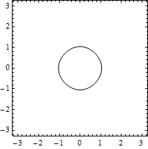
Figure 1. $d=2$, $\lambda=0.25$.

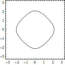
Figure 2. $d=2$, $\lambda=0.75$.

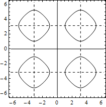
Figure 3. $d=2$, $\lambda=1.25$.

(2) The case $d=3$. By a direct computation, we have

$$\begin{split}&\det\Big{(}\delta_{ij}k_{3}^{2}\cos x_{j}+k_{i}k_{j}\cos x_{3}\Big{)}\\ &=k_{3}^{2}\left(k_{1}^{2}\cos x_{2}\cos x_{3}+k_{2}^{2}\cos x_{3}\cos x_{1}+k_{3}^{2}\cos x_{1}\cos x_{2}\right),\end{split}$$

which can vanish when e.g. $\cos x_{1}=\cos x_{2}=0$, $\cos x_{3}=1/2$. Therefore in 3-dimensions, $M_{\lambda}$ may not be convex. The following Figures 4, 5, 6 explain the situation in 3-dimensions.

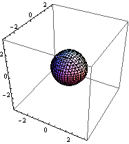
Figure 4. $d=3,\lambda=0.45$.

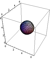
Figure 5. $d=3,\lambda=2.55$.

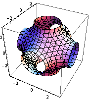
Figure 6. $d=3,\lambda=1.45$.

Here, we note the following simple lemma.

Lemma 4.2.

If $-1\leq y_{i}\leq 1$, $i=1,\cdots,d$, and $d-1<y_{1}+\cdots+y_{d}<d$, we have $y_{i}>0$, $i=1,\cdots d$.

Proof. Suppose e.g. $y_{d}\leq 0$. Then

$$y_{1}+y_{2}+\cdots+y_{d}\leq y_{1}+\cdots+y_{d-1}\leq d-1,$$

which is a contradiction. ∎

By (4.6), we have

$$\sum_{i,j=1}^{d-1}\frac{\partial^{2}\varphi}{\partial x_{i}\partial x_{j}}\xi_{i}\xi_{j}=-\frac{1}{(\sin x_{d})^{2}\rho}\left(k_{d}^{2}\sum_{i=1}^{d-1}\big{(}\cos x_{i}\big{)}\xi_{i}^{2}+\big{(}\cos x_{d}\big{)}\Big{(}\sum_{i=1}^{d-1}k_{i}\xi_{i}\Big{)}^{2}\right),$$

which has a definite sign if $\cos x_{i}>0$, $i=1,\cdots,d$ and $\sin x_{d}>0$. By virtue of Lemma 4.2, it happens for $0<\lambda<1/2$. Let us also note that for $d-1/2<\lambda<d$, we have the same conclusion since $\cos x_{i}<0\ (i=1,\cdots,d)$, $\sin x_{d}<0$. Recall that when $d\geq 3$ the definition of the Gaussian curvature depends on the choice of direction of the unit normal $N(x)$ on $S$. We choose $N(x)$ in such a way that $K(x)>0$ on $S$.

With this convention, we have proven the following lemma. Recall the interval $I_{d}$ defined by (1.6).

Lemma 4.3.

If $\lambda\in I_{d}$, all the principal curvature of $M_{\lambda}$ are positive.

As has been noted above, in the case $1<\lambda<2\ (d=2)$ or $d-1/2<\lambda<d\ (d\geq 3)$, we should shift the fundamental domain so that ${\bf R}^{d}/(2\pi{\bf Z})^{d}=[0,2\pi]^{d}$ (See Figures 3, 4, 5). To fix the idea, in the sequel, we deal with the case ${\bf R}^{d}/(2\pi{\bf Z})^{d}={\bf T}^{d}=[-\pi,\pi]^{d}$.

Under the assumption of Lemma 4.3, $M_{\lambda}$ is strictly convex. Let $N(x)$ be the unit normal field on $M_{\lambda}$ specified as above. Then for any $\omega\in S^{d-1}$, there exists a unique pair of points $x_{\pm}(\lambda,\omega)$ in $M_{\lambda}$ such that

(4.8) $$N(x_{\pm}(\lambda,\omega))=\pm\omega.$$

Since $N(-x)=-N(x)$, we see that $x_{-}(\lambda,\omega)=-x_{+}(\lambda,\omega)$. Therefore, we let

(4.9) $$x_{\pm}(\lambda,\omega)=\pm x_{\infty}(\lambda,\omega).$$

We can now compute the asymptotic expansion of the free resolvent

(4.10) $$\big{(}\widehat{R}_{0}(z)\widehat{f}\big{)}(m)=\sum_{n\in{\bf Z}^{d}}r_{0}(m-n,z)\widehat{f}(n),$$

(4.11) $$r_{0}(k,z)=(2\pi)^{-d}\int_{{\bf T}^{d}}\frac{e^{ik\cdot x}}{h(x)-z}dx.$$

We put

(4.12) $$\omega_{k}=k/|k|,\quad k\in{\bf R}^{d}\setminus\{0\}.$$

Lemma 4.4.

Assume $\lambda\in I_{d}$. Then we have as $|k|\to\infty$

$$\begin{split}&r_{0}(k,\lambda\pm i0)\\ =&\pm i(2\pi|k|)^{-(d-1)/2}e^{\pm i(k\cdot x_{\infty}(\lambda,\omega_{k})-(d-1)\pi/4)}\frac{K(x_{\pm}(\lambda,\omega_{k}))^{-1/2}}{|\nabla_{x}h(x_{\pm}(\lambda,\omega_{k}))|}+O(|k|^{-(d+1)/2}).\end{split}$$

Proof. Take $\epsilon>0$ small enough so that

$$(\lambda-2\epsilon,\lambda+2\epsilon)\subset\left\{\begin{split}&(0,1),\quad d=2,\\ &(0,1/2),\quad d\geq 3.\end{split}\right.$$

Let $\chi(t)\in C_{0}^{\infty}({\bf R})$ be such that $\chi(t)=1$ for $|t|<\epsilon/2$, $\chi(t)=0$ for $|t|>\epsilon$, and assume that $|{\rm Re}\,z-\lambda|<\epsilon/4$. We split $r_{0}(k,z)$ into two parts

$$r_{0}(k,z)=A(k,z)+B(k,z),$$

$$A(k,z)=(2\pi)^{-d}\int_{{\bf T}^{d}}\frac{\chi(h(x)-\lambda)}{h(x)-z}e^{ik\cdot x}dx.$$

Then, by integration by parts, for all $N>0$

$$B(k,z)=O(|k|^{-N}),\quad|k|\to\infty.$$

Letting $S(t)=\big{\{}x\in{\bf T}^{d}\,;\,h(x)=t\big{\}}$, we write $A(k,z)$ as

$$A(k,z)=(2\pi)^{-d}\int_{\lambda-\epsilon}^{\lambda+\epsilon}\frac{a(t,k)}{t-z}dt,\quad a(t,k)=\int_{S(t)}e^{ik\cdot x}\frac{\chi(t-\lambda)}{|\nabla_{x}h(x)|}dS(t).$$

We then have

(4.13) $$\int_{\lambda-\epsilon}^{\lambda+\epsilon}\frac{a(t,k)}{t-\lambda\mp i0}dt=\pm i\pi a(\lambda,k)+{\rm p.v.}\int_{\lambda-\epsilon}^{\lambda+\epsilon}\frac{a(t,k)}{t-\lambda}dt.$$

By Theorem 4.1, for $t\in(\lambda-\epsilon,\lambda+\epsilon)$, $a(t,k)$ admits the asymptotic expansion

$$a(t,k)=a_{0}(t,k)+O(|k|^{-(d+1)/2}),$$

(4.14) $$\begin{split}a_{0}(t,k)&=\Big{(}\frac{2\pi}{|k|}\Big{)}^{(d-1)/2}e^{ik\cdot x_{\infty}(t,\omega_{k})-(d-1)\pi i/4}\chi(t-\lambda)\frac{K(x_{+}(t,\omega_{k}))^{-1/2}}{|\nabla_{x}h(x_{+}(t,\omega_{k}))|}\\ &+\Big{(}\frac{2\pi}{|k|}\Big{)}^{(d-1)/2}e^{-ik\cdot x_{\infty}(t,\omega_{k})+(d-1)\pi i/4}\chi(t-\lambda)\frac{K(x_{-}(t,\omega_{k}))^{-1/2}}{|\nabla_{x}h(x_{-}(t,\omega_{k}))|}\\ &=:a_{0}^{(+)}(t,k)+a_{0}^{(-)}(t,k),\end{split}$$

where $x_{\pm}(t,\omega_{k})$ is a stationary phase point on $S(t)$.

We compute the asymptotic expansion of the 2nd term of the right-hand side of (4.13). Differentiating $h(x_{\pm}(t,\omega_{k}))=t$, we have

$$\nabla_{x}h(x_{\pm}(t,\omega_{k}))\cdot\partial_{t}x_{\pm}(t,\omega_{k})=1.$$

Therefore, letting

$$s=\omega_{k}\cdot x_{\pm}(t,\omega_{k})-\omega_{k}\cdot x_{\pm}(\lambda,\omega_{k}),$$

we have

$$\frac{ds}{dt}=\omega_{k}\cdot\partial_{t}x_{\pm}(t,\omega_{k})=\frac{\nabla_{x}h(x_{\pm}(t,\omega_{k}))}{|\nabla_{x}h(x_{\pm}(t,\omega_{k})|}\cdot\partial_{t}x_{\pm}(t,\omega_{k})=\frac{1}{|\nabla_{x}h(x_{\pm}(t,\omega_{k}))|},$$

which implies

$$t-\lambda=s|\nabla_{x}h(x_{\pm}(\lambda,\omega_{k}))|+O(s^{2}).$$

We then have

$$\frac{1}{t-\lambda}\frac{\chi(t-\lambda)K(x_{\pm}(t,\omega_{k}))^{-1/2}}{|\nabla_{x}h(x_{\pm}(t,\omega_{k})|}\frac{dt}{ds}=\frac{b_{\pm}(s,\omega_{k})}{s},$$

where $b_{\pm}(s,\omega_{k})$ is a smooth function such that

$$b_{\pm}(0,\omega_{k})=\frac{K(x_{\pm}(\lambda,\omega_{k}))^{-1/2}}{|\nabla_{x}h(x_{\pm}(\lambda,\omega_{k}))|}.$$

Taking $\delta>0$ small enough, we have by integration by parts

$$\begin{split}{\rm p.v.}\int_{-\delta}^{\delta}\frac{e^{\pm i|k|s}}{s}b_{\pm}(s,\omega_{k})ds&=\pm 2i\int_{0}^{|k|\delta}\frac{\sin s}{s}ds\,b_{\pm}(0,\omega_{k})+O(|k|^{-1})\\ &=\pm\pi i\,b_{\pm}(0,\omega_{k})+O(|k|^{-1}),\end{split}$$

which implies

(4.15) $$\begin{split}&{\rm p.v.}\int_{\lambda-\epsilon}^{\lambda+\epsilon}\frac{a_{0}^{(\pm)}(t,k)}{t-\lambda}dt\\ &=\Big{(}\frac{2\pi}{|k|}\Big{)}^{(d-1)/2}e^{\pm ik\cdot x_{\infty}(\lambda,\omega_{k})\mp(d-1)i\pi/4}{\rm p.v.}\int_{-\delta}^{\delta}\frac{e^{\pm i|k|s}}{s}b_{\pm}(s,\omega_{k})ds+O(|k|^{-(d+1)/2})\\ &=\pm i\pi\Big{(}\frac{2\pi}{|k|}\Big{)}^{(d-1)/2}e^{\pm ik\cdot x_{\infty}(\lambda,\omega_{k})\mp(d-1)i\pi/4}\frac{K(x_{\pm}(\lambda,\omega_{k}))^{1/2}}{|\nabla_{x}h(x_{\pm}(\lambda,\omega_{k}))|}+O(|k|^{-(d+1)/2}).\end{split}$$

Plugging (4.13), (4.14) and (4.15), we obtain the lemma. ∎

Lemma 4.5.

We have as $|m|\to\infty$

$$(m-n)\cdot x_{\pm}(\lambda,\omega_{m-n})=(m-n)\cdot x_{\pm}(\lambda,\omega_{m})+O(|m|^{-1}).$$

Proof. We extend $x_{\pm}(\lambda,k)$ as a function of homogeneous degree 0 in $k$. Letting $\epsilon=1/|m|$, we have

$$\omega_{m-n}=(\omega_{m}-\epsilon n)/|\omega_{m}-\epsilon n|=\omega_{m}+\epsilon((\omega_{m}\cdot n)\omega_{m}-n)+O(\epsilon^{2}).$$

Using $h(x_{\pm}(\lambda,\omega_{m-n}))=\lambda$, we have

$$\nabla_{x}h(x_{\pm}(\lambda,\omega_{m-n}))\cdot\frac{d}{d\epsilon}x_{\pm}(\lambda,\omega_{m-n})\Big{|}_{\epsilon=0}=0.$$

Since $\nabla_{x}h(x_{\pm}(\lambda,\omega))$ is parallel to $\omega$, we then have

$$\omega_{m}\cdot\frac{d}{d\epsilon}x_{\pm}(\lambda,\omega_{m-n})\Big{|}_{\epsilon=0}=0,$$

which implies

$$m\cdot x_{\pm}(\lambda,\omega_{m-n})=m\cdot x_{\pm}(\lambda,\omega_{m})+O(|m|^{-1}),$$

and the lemma follows immediately. ∎

Lemmas 4.4 and 4.5 imply the following lemma.

Lemma 4.6.

If $\lambda\in I_{d}$ and $\widehat{f}(n)$ is compactly supported, we have as $|k|\to\infty$

$$\begin{split}&\left(\widehat{R}_{0}(\lambda\pm i0)\widehat{f}\right)(k)\\ &=e^{\pm(3-d)\pi i/4}(2\pi|k|)^{-(d-1)/2}e^{\pm ik\cdot x_{\infty}(\lambda,\omega_{k})}a_{\pm}(\lambda,\omega_{k})\sum_{n}e^{\mp in\cdot x_{\infty}(\lambda,\omega_{k})}\widehat{f}(n)\\ &+O(|k|^{-(d+1)/2}),\end{split}$$

(4.16) $$a_{\pm}(\lambda,\omega_{k})=\frac{K(x_{\pm}(\lambda,\omega_{k}))^{-1/2}}{|\nabla_{x}h(x_{\pm}(\lambda,\omega_{k}))|}.$$

Recalling the definition of $x(\sqrt{\lambda}\theta)$ in (3.1) and the fact that the Gauss map is a diffeomorphism for a strictly convex surface, define $\theta(\lambda,\omega)$ by the relation $x(\sqrt{\lambda}\,\theta(\lambda,\omega))=x_{\infty}(\lambda,\omega)$, i.e.

(4.17) $$\theta_{j}(\lambda,\omega)=\frac{1}{\sqrt{\lambda}}\sin\Big{(}\frac{1}{2}\,x_{\infty j}(\lambda,\omega)\Big{)},\quad j=1,\cdots,d.$$

We define the reparametrized Fourier transforms $\widehat{\mathcal{G}}_{0}(\lambda)$ and $\widehat{\mathcal{G}}^{(\pm)}(\lambda)$ by

(4.18) $$\left(\widehat{\mathcal{G}}_{0}(\lambda)\widehat{f}\right)(\omega)=\left(\widehat{\mathcal{F}}_{0}(\lambda)\widehat{f}\right)(\theta(\lambda,\omega)),$$

(4.19) $$\widehat{\mathcal{G}}^{(\pm)}(\lambda)=\widehat{\mathcal{G}}_{0}(\lambda)(1-\widehat{V}\widehat{R}(\lambda\pm i0)).$$

Lemma 4.6, the definition (3.7) and the resolvent equation imply the following theorem.

Theorem 4.7.

If $\lambda\in I_{d}$ and $\widehat{f}(n)$ is compactly supported, we have as $|k|\to\infty$

$$\begin{split}&\left(\widehat{R}(\lambda\pm i0)\widehat{f}\right)(k)\\ =&\ e^{\pm(3-d)\pi i/4}\sqrt{2\pi}|k|^{-(d-1)/2}e^{\pm ik\cdot x_{\infty}(\lambda,\omega_{k})}a_{\pm}(\lambda,\omega_{k})\left(\widehat{\mathcal{G}}^{(\pm)}(\lambda)\widehat{f}\right)(\pm\omega_{k})\\ &+O(|k|^{-(d+1)/2}).\end{split}$$

5. Radiation conditions on ${\bf Z}^{d}$

The aim of this section is to introduce the radiation condition (Definition 5.5) and prove the uniqueness theorem (Theorem 5.9).

5.1. Green’s formula

For $m,n\in{\bf Z}^{d}$, we write $m\sim n$, if $|m-n|=1$, i.e. there exists $j$ such that $m=n\pm e_{j}$. We define the discrete Laplacian $\Delta_{disc}$ on ${\bf Z}^{d}$ by

(5.1) $$(\Delta_{disc}\widehat{u})(n)=-(\widehat{H}_{0}\widehat{u})(n)=\frac{1}{4}\sum_{m\sim n}\big{(}\widehat{u}(m)-\widehat{u}(n)\big{)}.$$

A set $D\subset{\bf Z}^{d}$ is said to be connected if for any $m,n\in D$, there exist $m^{(j)}\in D$, $j=0,\cdots,k$ such that $m^{(j)}\sim m^{(j+1)}$, $j=0,\cdots,k-1$, and $m^{(0)}=m$, $m^{(k)}=n$. A connected subset $D\subset{\bf Z}^{d}$ is called a domain. For a domain $D\subset{\bf Z}^{d}$, we define

(5.2) $${\rm deg}\,(n)=\,^{\#}\big{\{}m\in D\,;\,m\sim n\big{\}},\quad n\in D,$$

(5.3) $$\stackrel{{\scriptstyle\circ}}{{D}}\,=\big{\{}n\in D\,;\,{\rm deg}\,(n)=2d\big{\}},$$

(5.4) $$\partial D=\big{\{}n\in D\,;\,{\rm deg}\,(n)<2d\big{\}}.$$

The normal derivative at the boundary is defined by

(5.5) $$\left(\partial_{\nu}^{D}\widehat{u}\right)(n)=\frac{1}{4}\sum_{m\in\stackrel{{\scriptstyle\circ}}{{D}},m\sim n}\big{(}\widehat{u}(n)-\widehat{u}(m)\big{)},\quad n\in\partial D.$$

Note that, compared with (5.1), $m$ and $n$ are interchanged. Then the following Green’s formula holds (see e.g [5] and [11]):

(5.6) $$\begin{split}&\sum_{n\in\stackrel{{\scriptstyle\circ}}{{D}}}\big{(}(\Delta_{disc}\widehat{u})(n)\cdot\widehat{v}(n)-\widehat{u}(n)\cdot(\Delta_{disc}\widehat{u})(n)\big{)}\\ &=\sum_{n\in\partial D}\big{(}(\partial^{D}_{\nu}\widehat{u})(n)\cdot\widehat{v}(n)-\widehat{u}(n)\cdot(\partial^{D}_{\nu}\widehat{v})(n)\big{)}.\end{split}$$

5.2. Radiation condition

For $m,n$ such that $m\sim n$, we define the difference operator $\partial_{m-n}$ by

$$\big{(}\partial_{m-n}\widehat{f}\big{)}(n)=\widehat{f}(m)-\widehat{f}(n).$$

Lemma 5.1.

(1) Let $n(s)=n+s(m-n)$, where $m\sim n$. Then we have

$$\partial_{m-n}(n\cdot x_{\infty}(\lambda,\omega_{n}))=\int_{0}^{1}(m-n)\cdot x_{\infty}(\lambda,\omega_{n(s)})ds.$$

(2) If $m\sim n$, we have as $|n|\rightarrow\infty$

$$\partial_{m-n}(n\cdot x_{\infty}(\lambda,\omega_{n}))=(m-n)\cdot x_{\infty}(\lambda,\omega_{n})+O(|n|^{-1}),$$

$$\partial_{m-n}\left(e^{in\cdot x_{\infty}(\lambda,\omega_{n})}\right)=\left(e^{i(m-n)\cdot x_{\infty}(\lambda,\omega_{n})}-1\right)e^{in\cdot x_{\infty}(\lambda,\omega_{n})}+O(|n|^{-1}).$$

Proof. Differentiating $h(x_{\infty}(\lambda,\omega_{n(s)}))=\lambda$, we have

$$(\nabla_{x}h)(x_{\infty}(\lambda,\omega_{n(s)}))\cdot\frac{d}{ds}x_{\infty}(\lambda,\omega_{n(s)})=0.$$

Since $(\nabla_{x}h)(x_{\infty}(\lambda,\omega_{n(s)}))$ is parallel to $n(s)$, we then have

$$n(s)\cdot\frac{d}{ds}x_{\infty}(\lambda,\omega_{n(s)})=0,$$

which implies

$$\frac{d}{ds}(n(s)\cdot x_{\infty}(\lambda,\omega_{n(s)}))=(m-n)\cdot x_{\infty}(\lambda,\omega_{n(s)}).$$

Integrating this equality, we obtain (1). Since $\omega_{n(s)}=\omega_{n}+O(|n|^{-1})$, (2) follows from (1). ∎

We now introduce the rectangular domain $D(R)$ such that

(5.7) $$\stackrel{{\scriptstyle\circ}}{{D(R)}}=\big{\{}n\in{\bf Z}^{d}\ ;\ n\in[-R,R]^{d}\big{\}},\quad R>0,$$

and the radial derivative $\partial_{rad}$ by

(5.8) $$(\partial_{rad}\,\widehat{u})(k)=\frac{1}{4}\sum_{m\in\partial D(R(k)),m\sim k}(\widehat{u}(m)-\widehat{u}(k)),$$

(5.9) $$R(k)=\max_{1\leq j\leq d}\,|k_{j}|,\quad k\in{\bf Z}^{d}.$$

We put

(5.10) $$A_{\pm}(\lambda,\omega_{k})=\frac{1}{4}\sum_{m\in\partial D(R(k)),m\sim k}\left(e^{\pm i(m-k)\cdot x_{\infty}(\lambda,\omega_{k})}-1\right),\quad\omega_{k}=\frac{k}{|k|}.$$

Lemma 5.2.

(1) The right-hand side of (5.10) does not depend on $|k|$.
(2) There exists a constant $\epsilon_{0}(\lambda)>0$ such that

$$\pm\mathrm{Im}A_{\pm}(\lambda,\omega_{k})>\epsilon_{0}(\lambda),$$

for any $\omega_{k}$.

Proof. If $m\sim k$, $m\in\partial D(R(k))$, then $m-k=\pm e_{j}$ for some $j$. This $\pm e_{j}$ depends only on $\omega_{k}$, which proves (1).

Recall that $\nabla h(x)=\frac{1}{2}(\sin x_{1},\cdots,\sin x_{d})$, hence letting $\omega_{k,j}$ be the $j$-th component of $\omega_{k}$, we have

$$\sin(x_{\infty j}(\lambda,\omega_{k}))=c\omega_{k,j}$$

for some constant $c>0$. Suppose $m\sim k$, $m\in\partial D(R(k))$. If $\omega_{k,j}>0$, then either $m_{j}=k_{j}$ or $m_{j}=k_{j}+1$. If $\omega_{k,j}<0$, then either $m_{j}=k_{j}$ or $m_{j}=k_{j}-1$. We then have that $\sin((m-k)\cdot x_{\infty}(\lambda,\omega_{k}))=c|\omega_{k,j}|$ for some $j$ such that $\omega_{k,j}\not=0$. Since

$$\begin{split}\pm\mathrm{Im}A_{\pm}(\lambda,\omega_{k})&=\frac{1}{4}\sum_{m\in\partial D(R(k)),m\sim k}\sin((m-k)\cdot x_{\infty}(\lambda,\omega_{k}))\\ &=\frac{c}{4}\sum_{m\in\partial D(R(k)),m\sim k}|\omega_{k,j}|,\end{split}$$

and $\sum_{j}\omega_{k,j}^{2}=1$, the lemma follows. ∎

Let us introduce two auxiliary norms, $\widehat{\mathcal{B}}^{\ast}_{{\bf R}}$-norm and $\widehat{\mathcal{B}}^{\ast}_{{\bf Z}}$-norm, on $\widehat{\mathcal{B}}^{\ast}$ by

$$\|\widehat{u}\|^{2}_{\widehat{\mathcal{B}}^{\ast}_{{\bf R}}}=\sup_{R>1,R\in{\bf R}}\frac{1}{R}\sum_{n\in\stackrel{{\scriptstyle\circ}}{{D(R)}}}|\widehat{u}(n)|^{2},$$

$$\|\widehat{u}\|^{2}_{\widehat{\mathcal{B}}^{\ast}_{{\bf Z}}}=\sup_{\rho>1,\rho\in{\bf Z}}\frac{1}{\rho}\sum_{n\in\stackrel{{\scriptstyle\circ}}{{D(\rho)}}}|\widehat{u}(n)|^{2}.$$

Lemma 5.3.

These three norms $\|\cdot\|_{\widehat{\mathcal{B}}^{\ast}}$, $\|\cdot\|_{\widehat{\mathcal{B}}^{\ast}_{{\bf R}}}$, and $\|\cdot\|_{\widehat{\mathcal{B}}^{\ast}_{{\bf Z}}}$ are equivalent.

Proof. Let $A(R)=\{z\in{\bf C}^{d};(\sum_{j=1}^{d}|z_{j}|^{2})^{1/2}<R\}$, $B(R)=\{z\in{\bf C}^{d};\max_{j}|z_{j}|<R\}$. Then there is a constant $\delta>0$ such that $A(\delta R)\subset B(R)\subset A(R/\delta)$, $\forall R>0$. This implies

$$\frac{1}{R}\sum_{|n|<\delta R}|\widehat{u}(n)|^{2}\leq\frac{1}{R}\sum_{n\in\stackrel{{\scriptstyle\circ}}{{D(R)}}}|\widehat{u}(n)|^{2}\leq\frac{1}{R}\sum_{|n|<R/\delta}|\widehat{u}(n)|^{2}.$$

Taking the supremum with respect to $R>\delta$ or $R>1/\delta$, we get the equivalence of $\|\cdot\|_{\widehat{\mathcal{B}}^{\ast}}$ norm and $\|\cdot\|_{\widehat{\mathcal{B}}^{\ast}_{{\bf R}}}$ norm.

Next we show the equivalence of $\|\cdot\|_{\widehat{\mathcal{B}}^{\ast}_{{\bf R}}}$ norm and $\|\cdot\|_{\widehat{\mathcal{B}}^{\ast}_{{\bf Z}}}$ norm. Note that $f(r)=\sum_{n\in\stackrel{{\scriptstyle\circ}}{{D(r)}}}|\widehat{u}(n)|^{2}$ is a right-continuous non-decreasing step function on $(0,\infty)$ with jump at integers. For $R>1$, we take $\rho(R)=[R]$ = the largest positive integer such that $\rho(R)\leq R$. Then we have

$$\sup_{R>1}\frac{1}{R}\sum_{n\in\stackrel{{\scriptstyle\circ}}{{D(R)}}}|\widehat{u}(n)|^{2}\leq\sup_{R>1}\frac{1}{\rho(R)}\sum_{n\in\stackrel{{\scriptstyle\circ}}{{D(\rho(R))}}}|\widehat{u}(n)|^{2}.$$

The converse inequality is proven by the following inequality

$$\sup_{R>1}\frac{1}{\rho(R)}\sum_{n\in\stackrel{{\scriptstyle\circ}}{{D(\rho(R))}}}|\widehat{u}(n)|^{2}\leq\sup_{R>1}\frac{2}{R}\sum_{n\in\stackrel{{\scriptstyle\circ}}{{D(R)}}}|\widehat{u}(n)|^{2}.\qed$$

Lemma 5.4.

(1)  If $\widehat{f}\in\ell^{\infty}({\bf Z}^{d})$ satisfies $|\widehat{f}(n)|\leq C(1+|n|)^{-(d-1)/2}$, then

(5.11) $$\sup_{R>1}\frac{1}{R}\sum_{|n|<R}|\widehat{f}(n)|^{2}<\infty,\quad\text{i.e.}\quad\widehat{f}\in\widehat{\mathcal{B}}^{\ast}.$$

(2)  If $|\widehat{f}(n)|\leq C(1+|n|)^{-(d-1)/2-\epsilon}$, $\epsilon>0$, then

(5.12) $$\lim_{R\to\infty}\frac{1}{R}\sum_{|n|<R}|\widehat{f}(n)|^{2}=0.$$

Proof. We compute the norm $\|\widehat{f}\|_{\widehat{\mathcal{B}}^{\ast}_{{\bf Z}}}$. We first show

(5.13) $$\sum_{n\in\stackrel{{\scriptstyle\circ}}{{D(\rho)}}\setminus\stackrel{{\scriptstyle\circ}}{{D(\rho-1)}}}|\widehat{f}(n)|^{2}=O(1),$$

as $\rho\to\infty$. In fact, for any $\rho\in{\bf Z},\,\rho>1$ and $n\in\,\stackrel{{\scriptstyle\circ}}{{D(\rho)}}\setminus\stackrel{{\scriptstyle\circ}}{{D(\rho-1)}}$, we have $\rho-1<|n|\leq\sqrt{d}\rho$. Since ${}^{\#}\big{\{}n\in\,\stackrel{{\scriptstyle\circ}}{{D(\rho)}}\setminus\stackrel{{\scriptstyle\circ}}{{D(\rho-1)}}\big{\}}=(2\rho+1)^{d}-(2\rho-1)^{d}\leq C\rho^{d-1}$,

$$\sum_{n\in\stackrel{{\scriptstyle\circ}}{{D(\rho)}}\setminus\stackrel{{\scriptstyle\circ}}{{D(\rho-1)}}}|\widehat{f}(n)|^{2}\leq C\rho^{-(d-1)}\,{}^{\#}\big{\{}n\in\,\stackrel{{\scriptstyle\circ}}{{D(\rho)}}\setminus\stackrel{{\scriptstyle\circ}}{{D(\rho-1)}}\big{\}}\leq C.$$

On the other hand, since

$$\sum_{n\in\stackrel{{\scriptstyle\circ}}{{D(R)}}}|\widehat{f}(n)|^{2}=\sum_{\rho=1}^{R}\sum_{n\in\stackrel{{\scriptstyle\circ}}{{D(\rho)}}\setminus\stackrel{{\scriptstyle\circ}}{{D(\rho-1)}}}|\widehat{f}(n)|^{2}+|\widehat{f}(0)|^{2},$$

for every positive integer $R$, we have $\sum_{n\in\stackrel{{\scriptstyle\circ}}{{D(R)}}}|\widehat{f}(n)|^{2}=O(R)$ by (5.13). This proves (1) by Lemma 5.3.

Assume $|\widehat{f}(n)|\leq C(1+|n|)^{-(d-1)/2-\epsilon}$ for some $\epsilon>0$. By the similar computation, we have $\sum_{n\in\stackrel{{\scriptstyle\circ}}{{D(R)}}}|\widehat{f}(n)|^{2}=o(R)$, which proves (2). ∎

For $\widehat{f},\ \widehat{g}\in\widehat{\mathcal{B}}^{\ast}$, we write

(5.14) $$\widehat{f}\simeq\widehat{g}\Longleftrightarrow\lim_{R\to\infty}\frac{1}{R}\sum_{|n|<R}|\widehat{f}(n)-\widehat{g}(n)|^{2}=0.$$

As we have seen above, (5.14) is equivalent to

$$\lim_{R\to\infty}\frac{1}{R}\sum_{n\in\stackrel{{\scriptstyle\circ}}{{D(R)}}}|\widehat{f}(n)-\widehat{g}(n)|^{2}=0.$$

Now let us consider the equation on ${\bf Z}^{d}$:

(5.15) $$(\widehat{H}-\lambda)\widehat{u}=\widehat{f}.$$

Definition 5.5.

A solution $\widehat{u}(k)\in\widehat{\mathcal{B}}^{\ast}$ of (5.15) is said to be outgoing (for $+$) or incoming (for $-$) if it satisfies

(5.16) $$(\partial_{rad}\widehat{u})(k)\simeq A_{\pm}(\lambda,\omega_{k})\widehat{u}(k),$$

in the sense of (5.14).

Theorem 5.6.

Let $\lambda\in I_{d}$. If $\widehat{f}$ is compactly supported, $\widehat{R}(\lambda\pm i0)\widehat{f}$ is an outgoing (for $+$) or incoming (for $-$) solution of the equation $(\widehat{H}-\lambda)\widehat{u}=\widehat{f}$.

Proof. Since $x_{\infty}(\lambda,\omega_{k})$ is homogeneous of degree $0$ in $k$ (see also the proof of Lemma 4.5), we have as $|k|\rightarrow\infty$

$$x_{\infty}(\lambda,\omega_{k\pm e_{j}})=x_{\infty}(\lambda,\omega_{k})+O(|k|^{-1}).$$

Then we have for any fixed $n\in{\bf Z}^{d}$

(5.17) $$e^{\pm in\cdot x_{\infty}(\lambda,\omega_{k\pm e_{j}})}-e^{\pm in\cdot x_{\infty}(\lambda,\omega_{k})}=O(|k|^{-1}),\quad|k|\to\infty.$$

If $\widehat{f}$ is compactly supported, $\big{(}\widehat{\mathcal{G}}^{(\pm)}(\lambda)\widehat{f}\big{)}(\omega_{k})$ is smooth with respect to $k$, so that we have from (5.17)

(5.18) $$\partial_{m-k}\left(a_{\pm}(\lambda,\omega_{k})\big{(}\widehat{\mathcal{G}}^{(\pm)}(\lambda)\widehat{f}\big{)}(\pm\omega_{k})\right)=O(|k|^{-1}).$$

We put $\widehat{u}^{(\pm)}=\widehat{R}(\lambda\pm i0)\widehat{f}$. Theorem 4.7 yields

(5.19) $$\begin{split}&(\partial_{rad}\widehat{u}^{(\pm)})(k)\\ &=C_{\pm}|k|^{-(d-1)/2}\left(\sum_{m\in\partial D(R(k)),m\sim k}\big{(}\partial_{m-k}\Phi^{(\pm)}_{\lambda}\big{)}(k)\right)+O(|k|^{-(d+1)/2}),\end{split}$$

as $|k|\rightarrow\infty$, where

$$C_{\pm}=\frac{1}{4}e^{\pm(3-d)\pi i/4}\sqrt{2\pi},$$

$$\Phi^{(\pm)}_{\lambda}(k)=e^{\pm ik\cdot x_{\infty}(\lambda,\omega_{k})}a_{\pm}(\lambda,\omega_{k})\big{(}\widehat{\mathcal{G}}^{(\pm)}(\lambda)\widehat{f}\big{)}(\pm\omega_{k}).$$

Lemma 5.1 (2) and (5.18) imply the theorem. ∎

5.3. Rellich type theorem

The following is an analogue of the Rellich type theorem for Schrödinger operators in ${\bf R}^{d}$ ([18]).

Theorem 5.7.

Let $\lambda\in(0,d)\setminus{\bf Z}$. Suppose a sequence $\{\widehat{u}(n)\}$ defined for $|n|\geq R_{0}>0$ satisfies

$$(-\Delta_{disc}-\lambda)\widehat{u}=0,\quad|n|>R_{0},$$

$$\lim_{R\to\infty}\frac{1}{R}\sum_{R_{0}<|n|<R}|\widehat{u}(n)|^{2}=0.$$

Then there exists $R_{1}>R_{0}$ such that $\widehat{u}(n)=0$ for $|n|>R_{1}$.

For the proof, see [11], Theorem 1.1.

5.4. Uniqueness theorem

Theorem 5.8.

Let $\lambda\in I_{d}$, and suppose that $\widehat{f}$ is compactly supported. Let $\widehat{u}^{(\pm)}$ be the outgoing (for $+$) or incoming (for $-$) solution of the equation $(\widehat{H}-\lambda)\widehat{u}^{(\pm)}=\widehat{f}$. Then

$$(\widehat{u}^{(\pm)},\widehat{f})-(\widehat{f},\widehat{u}^{(\pm)})=2i\lim_{R\to\infty}\sum_{k\in\stackrel{{\scriptstyle\circ}}{{D(R)}}\setminus\stackrel{{\scriptstyle\circ}}{{D(R-1)}}}\mathrm{Im}A_{\pm}(\lambda,\omega_{k})|\widehat{u}^{(\pm)}(k)|^{2}.$$

Proof. By Green’s formula, we have

$$\begin{split}&\sum_{k\in\stackrel{{\scriptstyle\circ}}{{D(\rho)}}}\left((\Delta_{disc}\widehat{u}^{(\pm)})(k)\cdot\overline{\widehat{u}^{(\pm)}(k)}-\widehat{u}^{(\pm)}(k)\cdot\overline{(\Delta_{disc}\widehat{u}^{(\pm)})(k)}\right)\\ &=\sum_{k\in\partial D(\rho)}\left((\partial_{\nu}^{D(\rho)}\widehat{u}^{(\pm)})(k)\cdot\overline{\widehat{u}^{(\pm)}(k)}-\widehat{u}^{(\pm)}(k)\cdot\overline{(\partial_{\nu}^{D(\rho)}\widehat{u}^{(\pm)})(k)}\right).\end{split}$$

The left-hand side converges to $(\widehat{u}^{(\pm)},\widehat{f})-(\widehat{f},\widehat{u}^{(\pm)})$ by the equation. Changing the order of the summation,we can see that the right-hand side is equal to

$$\begin{split}&\frac{1}{4}\sum_{k\in\partial D(\rho)}\sum_{m\in\stackrel{{\scriptstyle\circ}}{{D(\rho)}},m\sim k}\left(\widehat{u}^{(\pm)}(k)\cdot\overline{\widehat{u}^{(\pm)}(m)}-\widehat{u}^{(\pm)}(m)\cdot\overline{\widehat{u}^{(\pm)}(k)}\right)\\ &=\sum_{m\in\stackrel{{\scriptstyle\circ}}{{D(\rho)}}\setminus\stackrel{{\scriptstyle\circ}}{{D(\rho-1)}}}\left((\partial_{rad}\widehat{u}^{(\pm)})(m)\cdot\overline{\widehat{u}^{(\pm)}(m)}-\widehat{u}^{(\pm)}(m)\cdot\overline{(\partial_{rad}\widehat{u}^{(\pm)})(m)}\right).\end{split}$$

As $\rho\to\infty$, we can replace $\partial_{rad}\widehat{u}^{(\pm)}$ by $A_{\pm}(\lambda,\omega_{k})\widehat{u}^{(\pm)}$, and prove the theorem. ∎

Theorem 5.9.

Let $\lambda\in I_{d}$. If $\widehat{f}$ is compactly supported, then the outgoing solution of (5.15) is unique and given by $\widehat{R}(\lambda+i0)\widehat{f}$. The incoming solution is also unique and given by $\widehat{R}(\lambda-i0)\widehat{f}$.

Proof. In view of Theorem 5.6, we have only to prove the uniqueness. Let $\widehat{u}$ be the outgoing solution of $(\widehat{H}-\lambda)\widehat{u}=0$. Then, by Theorem 5.8 and Lemma 5.2 (2), we have $\lim_{R\to\infty}\sum_{k\in\stackrel{{\scriptstyle\circ}}{{D(R)}}\setminus\stackrel{{\scriptstyle\circ}}{{D(R-1)}}}|\widehat{u}(k)|^{2}=0$. This implies

$$\lim_{R\to\infty}\frac{1}{R}\sum_{k\in\stackrel{{\scriptstyle\circ}}{{D(R)}}}|\widehat{u}(k)|^{2}=0,$$

i.e. $\widehat{u}\simeq 0$. We can then use the Theorem 5.7 and the unique continuation theorem (see [11], Theorem 2.1) to see that $\widehat{u}=0$. ∎

6. Exterior problem

6.1. Helmholtz equation in an exterior domain

Let $D(R)$ be a rectangular domain in (5.7), and take a sufficiently large integer $R_{0}>0$ such that

(6.1) $${\rm supp}\,\widehat{V}\subset\,\stackrel{{\scriptstyle\circ}}{{D(R_{0})}}.$$

We put

(6.2) $$\Omega_{int}=D(R_{0}),$$

(6.3) $$\Omega_{ext}={\bf Z}^{d}\setminus\stackrel{{\scriptstyle\circ}}{{\Omega}}_{int}.$$

Therefore $\stackrel{{\scriptstyle\circ}}{{\Omega}}_{int}=\,\stackrel{{\scriptstyle\circ}}{{D(R_{0})}}\,=[-R_{0},R_{0}]^{d}\cap{\bf Z}^{d}$, and

(6.4) $$\partial\Omega_{int}=\partial\Omega_{ext}=\bigcup_{j=1}^{d}\big{\{}n\,;\,|n_{i}|\leq R_{0},\ (i\neq j),\ |n_{j}|=R_{0}+1\big{\}}.$$

The spaces $\widehat{\mathcal{B}}$, $\widehat{\mathcal{B}}^{\ast}$ and $\widehat{\mathcal{H}}^{s}$ on $\stackrel{{\scriptstyle\circ}}{{\Omega}}_{ext}$ are defined in the same way as in the whole space. Let $\widehat{H}_{ext}=-\Delta_{disc}$ on $\Omega_{ext}$ with Dirichlet boundary condition.

Lemma 6.1.

(1) $\widehat{H}_{ext}$ is self-adjoint, and $\sigma(\widehat{H}_{ext})=[0,d].$
(2) $\ \sigma_{p}(\widehat{H}_{ext})\cap\left((0,d)\setminus{\bf Z}\right)=\emptyset.$

Proof. The assertion (1) follows from the standard perturbation theory, and (2) is proved in Theorem 2.4 of [11]. ∎

For the solution of the equation $(-\Delta_{disc}-\lambda)\widehat{u}=\widehat{f}$ in $\stackrel{{\scriptstyle\circ}}{{\Omega}}_{ext}$, the radiation condition is defined in the same way as in §5. The following theorem is proved in the same way as in Theorem 5.9.

Theorem 6.2.

Let $\lambda\in I_{d}$. Then the solution of the equation $(-\Delta_{disc}-\lambda)\widehat{u}=0$ in $\stackrel{{\scriptstyle\circ}}{{\Omega}}_{ext}$, satisfying the Dirichlet boundary contidion and the outgoing (or incoming) radiation condition vanishes identically on $\Omega_{ext}$.

We prove the limiting absorption principle for $\widehat{R}_{ext}(z)=(\widehat{H}_{ext}-z)^{-1}$.

Theorem 6.3.

(1) For $\lambda\in I_{d}$ and $\widehat{f}\in\widehat{\mathcal{B}}$, the weak $\ast$-limit exists

$$\lim_{\epsilon\to 0}\widehat{R}_{ext}(\lambda\pm i\epsilon)\widehat{f}=:\widehat{R}_{ext}(\lambda\pm i0)\widehat{f}\in\widehat{\mathcal{B}}^{\ast}.$$

(2) For any compact set $J\subset I_{d}$, there exists a constant $C>0$ such that

$$\|\widehat{R}_{ext}(\lambda\pm i0)\widehat{f}\|_{\widehat{\mathcal{B}}^{\ast}}\leq C\|\widehat{f}\|_{\widehat{\mathcal{B}}},\quad\lambda\in J.$$

(3) For $\widehat{f},\,\widehat{g}\in\widehat{\mathcal{B}}$,

$$I_{d}\ni\lambda\mapsto\big{(}\widehat{R}_{ext}(\lambda\pm i0)\widehat{f},\,\widehat{g}\big{)}$$

is continuous.
(4) If $\widehat{f}$ is compactly supported, $\widehat{R}_{ext}(\lambda\pm i0)\widehat{f}$ satisfies the outgoing (for $+$) or incoming (for $-$) radiation condition.

Proof. We prove the theorem for $\lambda+i0$. We extend $\widehat{f}\in\widehat{\mathcal{B}}$ and $\widehat{u}(z)=\widehat{R}_{ext}(z)\widehat{f}$ to be 0 outside $\Omega_{ext}$. Then it satisfies

$$(\widehat{H}_{0}-z)\widehat{u}(z)=\widehat{K}\widehat{u}(z)+\widehat{f}\quad\text{on}\quad{\bf Z}^{d},$$

where $\widehat{K}=\sum_{n}c_{n}\widehat{P}(n)$ is a finite sum of projections $\widehat{P}(n)$ to the site $n$. Therefore

(6.5) $$\widehat{u}(z)=\widehat{R}_{0}(z)\widehat{K}\widehat{u}(z)+\widehat{R}_{0}(z)\widehat{f}.$$

Let $J$ be a compact set in $I_{d}$, and take $s>1/2$. We first show that there exists a constant $C>0$ such that

(6.6) $$\|\widehat{u}(\lambda+i\epsilon)\|_{\widehat{\mathcal{H}}^{-s}}\leq C\|\widehat{f}\|_{\widehat{\mathcal{B}}},\quad\forall\lambda\in J,\quad\forall\epsilon>0.$$

In fact, if this does not hold, there exists $z_{\mu}=\lambda_{\mu}+i\epsilon_{\mu}$, $\widehat{f}_{\mu}\in\widehat{\mathcal{B}}$, such that $\widehat{u}_{\mu}=\widehat{R}_{ext}(z_{\mu})\widehat{f}_{\mu}$ satisfies

(6.7) $$z_{\mu}\to\lambda\in J,\quad\|\widehat{f}_{\mu}\|_{\widehat{\mathcal{B}}}\to 0,\quad\|\widehat{u}_{\mu}\|_{\widehat{\mathcal{H}}^{-s}}=1\quad\text{as}\quad\mu\to\infty.$$

One can then select a subsequence, which is denoted by $\{\widehat{u}_{\mu}\}$ again, such that $\widehat{u}_{\mu}$ converges weakly in $\widehat{\mathcal{H}}^{-s}$. Since $\widehat{K}$ is a finite dimensional operator, $\widehat{K}\widehat{u}_{\mu}$ converges in $\widehat{\mathcal{B}}$. Therefore, in view of (6.5), we see that $\widehat{u}_{\mu}$ converges in $\widehat{\mathcal{B}}^{\ast}$, hence in $\widehat{\mathcal{H}}^{-s}$, to $\widehat{u}$ such that $\|\widehat{u}\|_{\widehat{\mathcal{H}}^{-s}}=1$. It satisfies

$$(\widehat{H}_{ext}-\lambda)\widehat{u}=0,\quad\widehat{u}=\widehat{R}_{0}(\lambda+i0)\widehat{K}\widehat{u}.$$

Therefore $\widehat{u}$ is an outgoing solution. By Theorem 6.2, $\widehat{u}=0$, which is a contradiction.

We next prove that for $s>1/2$ and $\widehat{f}\in\widehat{\mathcal{B}}$, $\widehat{R}_{ext}(\lambda+i\epsilon)\widehat{f}$ converges strongly in $\widehat{\mathcal{H}}^{-s}$ as $\epsilon\to 0$. To prove it, we consider a sequence $u_{\mu}=\widehat{R}_{ext}(\lambda+i\epsilon_{\mu})\widehat{f}$, $\epsilon_{\mu}\to 0$. Then by the same arguments as above, one can show that any subsequence of $\{u_{\mu}\}$ contains a sub-subsequence $\{u_{\mu^{\prime}}\}$, which converges in $\mathcal{H}^{-s}$ to one and the same limit (independent of the choice of sub-subsequence). This proves the convergence of $\widehat{R}_{ext}(\lambda+i\epsilon)\widehat{f}$ as $\epsilon\to 0$. Arguing similarly, one can also show that

$$I_{d}\ni\lambda\mapsto\widehat{R}_{ext}(\lambda+i0)\widehat{f}\in\widehat{\mathcal{H}}^{-s}$$

is strongly continuous. The assertions of the theorem then follow from those for $\widehat{R}_{0}(\lambda+i0)$ and the formula

$$\widehat{R}_{ext}(\lambda+i0)=\widehat{R}_{0}(\lambda+i0)\big{(}1+\widehat{K}\widehat{R}_{ext}(\lambda+i0)\big{)}.\qed$$

6.2. Exterior and interior D-N maps

Let $\widehat{H}_{int}=-\Delta_{disc}+\widehat{V}$ be defined on $\Omega_{int}$ with Dirichlet boundary condition. The interior D-N map is defined by

(6.8) $$\Lambda_{\widehat{V}}(\lambda)\widehat{f}=\partial_{\nu}^{\Omega_{int}}\widehat{u}_{int}\Big{|}_{\partial\Omega_{int}},\quad\lambda\not\in\sigma(\widehat{H}_{int}),$$

where $\widehat{u}_{int}$ is the solution of the equation

(6.9) $$(-\Delta_{disc}+\widehat{V}-\lambda)\widehat{u}_{int}=0\quad\text{in}\quad\stackrel{{\scriptstyle\circ}}{{\Omega}}_{int},\quad\widehat{u}_{int}\Big{|}_{\partial\Omega_{int}}=\widehat{f}.$$

The exterior D-N map is defined by

(6.10) $$\Lambda_{ext}^{(\pm)}(\lambda)\widehat{f}=-\partial_{\nu}^{\Omega_{ext}}\widehat{u}_{ext}^{(\pm)}\Big{|}_{\partial\Omega_{ext}},\quad\lambda\in I_{d},$$

where $\widehat{u}_{ext}^{(\pm)}\in\widehat{\mathcal{B}}^{\ast}$ is the unique outgoing (for $+$) and incoming (for $-$) solution of the equation

(6.11) $$(\widehat{H}_{ext}-\lambda)\widehat{u}_{ext}^{(\pm)}=0\quad\text{in}\quad\stackrel{{\scriptstyle\circ}}{{\Omega}}_{ext},\quad\widehat{u}_{ext}^{(\pm)}\Big{|}_{\partial\Omega_{ext}}=\widehat{f}.$$

The existence of $\widehat{u}_{ext}^{(\pm)}$ is shown by extending $\widehat{f}$ to be zero on ${\bf Z}^{d}\setminus\partial\Omega_{ext}$, and putting

$$\widehat{u}_{ext}^{(\pm)}=\widehat{f}-\widehat{R}_{ext}(\lambda\pm i0)(-\Delta_{disc}-\lambda)\widehat{f}.$$

The uniqueness follows from Theorem 6.2.

We represent $\widehat{u}_{ext}^{(\pm)}$ in terms of exterior and interior D-N maps. In the following, for a subset $A$ in ${\bf Z}^{d}$, we use $\chi_{A}$ to mean either the operator of restriction

(6.12) $$\chi_{A}:\ell^{\infty}({\bf Z}^{d})\ni\widehat{f}\mapsto\widehat{f}\Big{|}_{A},$$

or the operator of extension

(6.13) $$\chi_{A}:\ell^{\infty}(A)\ni\widehat{f}\mapsto\left\{\begin{array}[]{cl}\widehat{f},&{\rm on}\quad A,\\ 0,&{\rm on}\quad{\bf Z}^{d}\setminus A,\end{array}\right.$$

which will not confuse our argument. We put

$$C(R_{0})=\partial\Omega_{int}=\partial\Omega_{ext}=\Omega_{int}\cap\Omega_{ext},$$

(6.14) $$\widehat{S}_{C(R_{0})}=\frac{1}{4}\sum_{j=1}^{d}\chi_{C(R_{0})}\big{(}\widehat{S}_{j}+(\widehat{S}_{j})^{\ast}\big{)}\chi_{C(R_{0})},$$

$$(\widehat{S}_{j}\widehat{u})(n)=\widehat{u}(n+e_{j}),\quad((\widehat{S}_{j})^{\ast}\widehat{u})(n)=\widehat{u}(n-e_{j}),$$

and also for $n\in C(R_{0})$

(6.15) $$\widetilde{\mathrm{deg}}_{C(R_{0})}(n)=\frac{1}{4}\,^{\#}\big{\{}m\in C(R_{0})\ ;\ |m-n|=1\big{\}}.$$

For $\lambda\in I_{d}\setminus\sigma(\widehat{H}_{int})$, we define the operator $B_{C(R_{0})}^{(\pm)}(\lambda)\in{\bf B}(\ell^{2}(C(R_{0})))$ by

(6.16) $$B_{C(R_{0})}^{(\pm)}(\lambda)=\Lambda_{\widehat{V}}(\lambda)-\Lambda_{ext}^{(\pm)}(\lambda)-\lambda+\frac{1}{4}\widetilde{\mathrm{deg}}_{C(R_{0})}-\widehat{S}_{C(R_{0})},$$

where $\widetilde{\mathrm{deg}}_{C(R_{0})}$ is the operator of multiplication by $\widetilde{\mathrm{deg}}_{C(R_{0})}(n)$.

Lemma 6.4.

Assume that $\lambda\in I_{d}\setminus\sigma(\widehat{H}_{int})$, $\widehat{f}\in\ell^{2}(C(R_{0}))$. Let $\widehat{u}^{(\pm)}_{ext}$ and $\widehat{u}_{int}$ be the solutions of (6.11) and (6.9), respectively, and put

$$\widehat{u}^{(\pm)}=\chi_{\stackrel{{\scriptstyle\circ}}{{\Omega}}_{int}}\widehat{u}_{int}+\chi_{\stackrel{{\scriptstyle\circ}}{{\Omega}}_{ext}}\widehat{u}_{ext}^{(\pm)}+\chi_{C(R_{0})}\widehat{f}.$$

Then we have

(6.17) $$\widehat{u}^{(\pm)}(n)=(\widehat{R}(\lambda\pm i0)\chi_{C(R_{0})}B_{C(R_{0})}^{(\pm)}(\lambda)\widehat{f})(n),\quad n\in{\bf Z}^{d}.$$

In particular,

(6.18) $$\widehat{u}_{ext}^{(\pm)}(n)=(\widehat{R}(\lambda\pm i0)\chi_{C(R_{0})}B_{C(R_{0})}^{(\pm)}(\lambda)\widehat{f})(n),\quad n\in\,\stackrel{{\scriptstyle\circ}}{{\Omega}}_{ext},$$

(6.19) $$\widehat{f}(n)=(\widehat{R}(\lambda\pm i0)\chi_{C(R_{0})}B_{C(R_{0})}^{(\pm)}(\lambda)\widehat{f})(n),\quad n\in C(R_{0}).$$

Proof. Let $\widehat{r}(n,m;\lambda\pm i0)$ be the resolvent kernel, i.e.

$$\widehat{r}(n,m;\lambda\pm i0)=\left(\widehat{R}(\lambda\pm i0)\widehat{\delta}_{m}\right)(n),$$

where $\widehat{\delta}_{m}(n)=\delta_{mn}$. As in the proof of Theorem 5.8, by Green’s formula,

(6.20) $$\begin{split}&\sum_{n\in(\stackrel{{\scriptstyle\circ}}{{\Omega}}_{int}\cup\stackrel{{\scriptstyle\circ}}{{\Omega}}_{ext})\cap\stackrel{{\scriptstyle\circ}}{{D(R)}}}\left((\Delta_{disc}\widehat{u}^{(\pm)})(n)\widehat{r}(n,m;\lambda\pm i0)-\widehat{u}^{(\pm)}(n)(\Delta_{disc}\widehat{r})(n,m;\lambda\pm i0)\right)\\ &=\sum_{n\in\partial\Omega_{int}}\left((\partial_{\nu}^{\Omega_{int}}\widehat{u}^{(\pm)})(n)\widehat{r}(n,m;\lambda\pm i0)-\widehat{u}^{(\pm)}(n)(\partial_{\nu}^{\Omega_{int}}\widehat{r})(n,m;\lambda\pm i0)\right)\\ &\quad+\sum_{n\in\partial\Omega_{ext}}\left((\partial_{\nu}^{\Omega_{ext}}\widehat{u}^{(\pm)})(n)\widehat{r}(n,m;\lambda\pm i0)-\widehat{u}^{(\pm)}(n)(\partial_{\nu}^{\Omega_{ext}}\widehat{r})(n,m;\lambda\pm i0)\right)\\ &\quad+\sum_{n\in\stackrel{{\scriptstyle\circ}}{{D(R)}}\setminus\stackrel{{\scriptstyle\circ}}{{D(R-1)}}}\left((\partial_{rad}\widehat{u}^{(\pm)})(n)\widehat{r}(n,m;\lambda\pm i0)-\widehat{u}^{(\pm)}(n)(\partial_{rad}\widehat{r})(n,m;\lambda\pm i0)\right),\end{split}$$

for sufficiently large integer $R>0$. By the equations (6.9) and (6.11), the left-hand side of (6.20) is equal to

(6.21) $$\begin{split}&\sum_{n\in(\stackrel{{\scriptstyle\circ}}{{\Omega}}_{int}\cup\stackrel{{\scriptstyle\circ}}{{\Omega}}_{ext})\cap\stackrel{{\scriptstyle\circ}}{{D(R)}}}\widehat{u}^{(\pm)}(n)((-\Delta_{disc}+\widehat{V}-\lambda)\widehat{r})(n,m;\lambda\pm i0)\\ &=\sum_{n\in(\stackrel{{\scriptstyle\circ}}{{\Omega}}_{int}\cup\stackrel{{\scriptstyle\circ}}{{\Omega}}_{ext})\cap\stackrel{{\scriptstyle\circ}}{{D(R)}}}\widehat{u}^{(\pm)}(n)\delta_{nm},\end{split}$$

for any $m\in{\bf Z}^{d}$. Note that, by our definitions of $\Lambda_{\widehat{V}}(\lambda)$ and $\Lambda_{ext}^{(\pm)}(\lambda)$,

$$\partial_{\nu}^{\Omega_{int}}\widehat{u}^{(\pm)}=\partial_{\nu}^{\Omega_{int}}\widehat{u}_{int}=\Lambda_{\widehat{V}}(\lambda)\widehat{f},$$

$$\partial_{\nu}^{\Omega_{ext}}\widehat{u}^{(\pm)}=\partial_{\nu}^{\Omega_{ext}}\widehat{u}_{ext}^{(\pm)}=-\Lambda_{ext}^{(\pm)}(\lambda)\widehat{f}.$$

The sum $\sum_{n\in\partial\Omega_{int}}+\sum_{n\in\partial\Omega_{ext}}$ in the right-hand side of (6.20) is then equal to

(6.22) $$\begin{split}&\sum_{n\in C(R_{0})}\left((\Lambda_{\widehat{V}}(\lambda)\widehat{f})(n)\widehat{r}(n,m;\lambda\pm i0)-\widehat{f}(n)(\partial_{\nu}^{\Omega_{int}}\widehat{r})(n,m;\lambda\pm i0)\right)\\ &\quad-\sum_{n\in C(R_{0})}\left((\Lambda_{ext}^{(\pm)}(\lambda)\widehat{f})(n)\widehat{r}(n,m;\lambda\pm i0)+\widehat{f}(n)(\partial_{\nu}^{\Omega_{ext}}\widehat{r})(n,m;\lambda\pm i0)\right)\\ &=\sum_{n\in C(R_{0})}\widehat{r}(n,m;\lambda\pm i0)\chi_{C(R_{0})}(n)\left((\Lambda_{\widehat{V}}(\lambda)-\Lambda_{ext}^{(\pm)}(\lambda))\widehat{f}\right)(n)\\ &\quad-\sum_{n\in C(R_{0})}\widehat{f}(n)\left((\partial_{\nu}^{\Omega_{int}}+\partial_{\nu}^{\Omega_{ext}})\widehat{r}\right)(n,m;\lambda\pm i0).\end{split}$$

For $n\in C(R_{0})$,

$$\begin{split}&\left((\partial_{\nu}^{\Omega_{int}}+\partial_{\nu}^{\Omega_{ext}})\widehat{r}\right)(n,m;\lambda\pm i0)\\ =&\frac{1}{4}\sum_{k\in\stackrel{{\scriptstyle\circ}}{{\Omega}}_{int}\cup\stackrel{{\scriptstyle\circ}}{{\Omega}}_{ext},k\sim n}\big{(}\widehat{r}(n,m;\lambda\pm i0)-\widehat{r}(k,m;\lambda\pm i0)\big{)}\\ =&-(\Delta_{disc}\widehat{r})(n,m;\lambda\pm i0)-\frac{1}{4}\sum_{k\in C(R_{0}),k\sim n}\big{(}\widehat{r}(n,m;\lambda\pm i0)-\widehat{r}(k,m;\lambda\pm i0)\big{)}.\end{split}$$

Therefore, the second term of the right-hand side of (6.22) is computed as follows:

$$\begin{split}&-\sum_{n\in C(R_{0})}\widehat{f}(n)\ (-\Delta_{disc}\widehat{r})(n,m;\lambda\pm i0)\\ &\quad+\frac{1}{4}\sum_{n\in C(R_{0})}\widehat{f}(n)\Big{(}\sum_{k\in C(R_{0}),k\sim n}\big{(}\widehat{r}(n,m;\lambda\pm i0)-\widehat{r}(k,m;\lambda\pm i0)\big{)}\Big{)}\\ &=-\sum_{n\in C(R_{0})}\widehat{f}(n)\delta_{nm}+\sum_{n\in C(R_{0})}\big{(}-\lambda+\frac{1}{4}\widetilde{\mathrm{deg}}_{C(R_{0})}(n)\big{)}\widehat{f}(n)\ \widehat{r}(n,m;\lambda\pm i0)\\ &\quad-\frac{1}{4}\sum_{k\in C(R_{0})}\widehat{r}(k,m;\lambda\pm i0)\sum_{n\in C(R_{0}),n\sim k}\widehat{f}(n),\end{split}$$

where, in the 3rd line, we have used the fact that

$$\big{(}(-\Delta_{disc}-\lambda)\widehat{r}\big{)}(n,m;\lambda\pm i0)=\delta_{nm},\quad n,m\in{\bf Z}^{d},$$

and exchanged the order of summation in the 4th line. Note that

$$\sum_{n\in C(R_{0}),n\sim k}\widehat{f}(n)=\sum_{j=1}^{d}\big{(}(\widehat{S}_{j}+(\widehat{S}_{j})^{\ast})\chi_{C(R_{0})}\widehat{f}\big{)}(k).$$

Since we have for any $m\in\,\stackrel{{\scriptstyle\circ}}{{D(R)}}$

$$\sum_{n\in(\stackrel{{\scriptstyle\circ}}{{\Omega}}_{int}\cup\stackrel{{\scriptstyle\circ}}{{\Omega}}_{ext})\cap\stackrel{{\scriptstyle\circ}}{{D(R)}}}\widehat{u}^{(\pm)}(n)\delta_{nm}+\sum_{n\in C(R_{0})}\widehat{f}(n)\delta_{nm}=\widehat{u}^{(\pm)}(m),$$

(6.20) turns out to be

$$\begin{split}&\widehat{u}^{(\pm)}(m)=\sum_{n\in C(R_{0})}\widehat{r}(n,m;\lambda\pm i0)\big{(}(\Lambda_{\widehat{V}}(\lambda)-\Lambda_{ext}^{(\pm)}(\lambda))\widehat{f}\big{)}(n)\\ &\ \ \ \ \ \ \ \ \ \ \ \ \ \ +\sum_{n\in C(R_{0})}\big{(}-\lambda+\frac{1}{4}\widetilde{\mathrm{deg}}_{C(R_{0})}(n)\big{)}\widehat{f}(n)\ \widehat{r}(n,m;\lambda\pm i0)\\ &\ \ \ \ \ \ \ \ \ \ \ \ \ \ -\frac{1}{4}\sum_{n\in C(R_{0})}\widehat{r}(n,m;\lambda\pm i0)\sum_{j=1}^{d}\big{(}(\widehat{S}_{j}+(\widehat{S}_{j})^{\ast})\chi_{C(R_{0})}\widehat{f}\big{)}(n)\\ &\quad+\sum_{n\in\stackrel{{\scriptstyle\circ}}{{D(R)}}\setminus\stackrel{{\scriptstyle\circ}}{{D(R-1)}}}\left((\partial_{rad}\widehat{u}^{(\pm)})(n)\widehat{r}(n,m;\lambda\pm i0)-\widehat{u}^{(\pm)}(n)(\partial_{rad}\widehat{r})(n,m;\lambda\pm i0)\right),\end{split}$$

for any $m\in\,\stackrel{{\scriptstyle\circ}}{{D(R)}}$. In view of (6.16), we have thus arrived at

$$\begin{split}&\widehat{u}^{(\pm)}(m)=\big{(}\widehat{R}(\lambda\pm i0)\chi_{C(R_{0})}B^{(\pm)}_{C(R_{0})}(\lambda)\widehat{f}\big{)}(m)\\ &\quad+\sum_{n\in\stackrel{{\scriptstyle\circ}}{{D(R)}}\setminus\stackrel{{\scriptstyle\circ}}{{D(R-1)}}}\left((\partial_{rad}\widehat{u}^{(\pm)})(n)\widehat{r}(n,m;\lambda\pm i0)-\widehat{u}^{(\pm)}(n)(\partial_{rad}\widehat{r})(n,m;\lambda\pm i0)\right).\end{split}$$

Taking the average of the sum with respect to $R$ in the above equality, we have

(6.23) $$\begin{split}\widehat{u}^{(\pm)}(m)&=\big{(}\widehat{R}(\lambda\pm i0)\chi_{C(R_{0})}B^{(\pm)}_{C(R_{0})}(\lambda)\widehat{f}\big{)}(m)\\ &+\frac{1}{R}\sum_{n\in\stackrel{{\scriptstyle\circ}}{{D(R)}}}\big{(}(\partial_{rad}-A_{\pm}(\lambda,\omega_{n}))\widehat{u}^{(\pm)}\big{)}(n)\widehat{r}(n,m;\lambda\pm i0)\\ &-\frac{1}{R}\sum_{n\in\stackrel{{\scriptstyle\circ}}{{D(R)}}}\widehat{u}^{(\pm)}(n)\big{(}(\partial_{rad}-A_{\pm}(\lambda,\omega_{n}))\widehat{r}\big{)}(n,m;\lambda\pm i0),\end{split}$$

up to a term of $O(R^{-1})$. By the radiation condition, we have

$$\begin{split}\frac{1}{R}&\left|\sum_{n\in\stackrel{{\scriptstyle\circ}}{{D(R)}}}\big{(}(\partial_{rad}-A_{\pm}(\lambda,\omega_{n}))\widehat{u}^{(\pm)}\big{)}(n)\widehat{r}(n,m;\lambda\pm i0)\right|\\ &\leq\left(\frac{1}{R}\sum_{n\in\stackrel{{\scriptstyle\circ}}{{D(R)}}}\big{|}\big{(}(\partial_{rad}-A_{\pm}(\lambda,\omega_{n}))\widehat{u}^{(\pm)}\big{)}(n)\big{|}^{2}\right)^{1/2}\\ &\quad\times\left(\frac{1}{R}\sum_{n\in\stackrel{{\scriptstyle\circ}}{{D(R)}}}|\widehat{r}(n,m;\lambda\pm i0)|^{2}\right)^{1/2},\end{split}$$

which tends to zero as $R\rightarrow\infty$. The third term of the right-hand side of (6.23) is estimated similarly. This proves the lemma. ∎

Lemma 6.5.

Suppose $\lambda\in I_{d}\setminus\sigma(\widehat{H}_{int})$. Then for $\widehat{f},\,\widehat{g}\in\ell^{2}(C(R_{0}))$, we have

(6.24) $$\big{(}\Lambda_{\widehat{V}}(\lambda)\widehat{f},\,\widehat{g}\big{)}_{\ell^{2}(C(R_{0}))}=\big{(}\widehat{f},\,\Lambda_{\widehat{V}}(\lambda)\widehat{g}\big{)}_{\ell^{2}(C(R_{0}))},$$

(6.25) $$\big{(}\Lambda_{ext}^{(\pm)}(\lambda)\widehat{f},\,\widehat{g}\big{)}_{\ell^{2}(C(R_{0}))}=\big{(}\widehat{f},\,\Lambda_{ext}^{(\mp)}(\lambda)\widehat{g}\big{)}_{\ell^{2}(C(R_{0}))}.$$

Proof. The first equality (6.24) follows from Green’s formula. We shall prove (6.25). Let $\widehat{u}$ be the outgoing solution of (6.11), and $\widehat{v}$ the incoming solution of (6.11) with $\widehat{f}$ replaced by $\widehat{g}$. For a sufficiently large integer $R>0$, we have by Green’s formula

$$\begin{split}0&=\sum_{n\in(D(R)\cap\Omega_{ext})^{\circ}}\left(((\widehat{H}_{ext}-\lambda)\widehat{u})(n)\cdot\overline{\widehat{v}(n)}-\widehat{u}(n)\cdot\overline{((\widehat{H}_{ext}-\lambda)\widehat{v})(n)}\right)\\ &=\sum_{n\in\partial D(R)}\left(-(\partial_{\nu}^{D(R)}\widehat{u})(n)\cdot\overline{\widehat{v}(n)}+\widehat{u}(n)\cdot\overline{(\partial_{\nu}^{D(R)}\widehat{v})(n)}\right)\\ &\quad+\sum_{n\in\partial\Omega_{ext}}\left(-(\partial_{\nu}^{\Omega_{ext}}\widehat{u})(n)\cdot\overline{\widehat{v}(n)}+\widehat{u}(n)\cdot\overline{(\partial_{\nu}^{\Omega_{ext}}\widehat{v})(n)}\right).\end{split}$$

As in the proof of Theorem 5.8, we have

$$\begin{split}&\sum_{n\in\partial D(R)}\left(-(\partial_{\nu}^{D(R)}\widehat{u})(n)\cdot\overline{\widehat{v}(n)}+\widehat{u}(n)\cdot\overline{(\partial_{\nu}^{D(R)}\widehat{v})(n)}\right)\\ &=\sum_{n\in\stackrel{{\scriptstyle\circ}}{{D(R)}}\setminus\stackrel{{\scriptstyle\circ}}{{D(R-1)}}}\left(-(\partial_{rad}\,\widehat{u})(n)\cdot\overline{\widehat{v}(n)}+\widehat{u}(n)\cdot\overline{(\partial_{rad}\,\widehat{v}(n)}\right).\end{split}$$

This implies

$$\begin{split}&\big{(}\Lambda_{ext}^{(+)}(\lambda)\widehat{f},\,\widehat{g}\big{)}_{\ell^{2}(\partial\Omega_{ext})}-\big{(}\widehat{f},\,\Lambda_{ext}^{(-)}(\lambda)\widehat{g}\big{)}_{\ell^{2}(\partial\Omega_{ext})}\\ &=\sum_{n\in\stackrel{{\scriptstyle\circ}}{{D(R)}}\setminus\stackrel{{\scriptstyle\circ}}{{D(R-1)}}}\big{(}(\partial_{rad}\,\widehat{u})(n)-A_{+}(\lambda,\omega_{n})\widehat{u}(n)\big{)}\overline{\widehat{v}(n)}\\ &\quad-\sum_{n\in\stackrel{{\scriptstyle\circ}}{{D(R)}}\setminus\stackrel{{\scriptstyle\circ}}{{D(R-1)}}}\widehat{u}(n)\overline{\big{(}(\partial_{rad}\,\widehat{v})(n)-A_{-}(\lambda,\omega_{n})\widehat{v}(n)\big{)}}.\end{split}$$

Then, taking the average of the sum with respect to $R$, we have

$$\begin{split}&\big{(}\Lambda_{ext}^{(+)}(\lambda)\widehat{f},\,\widehat{g}\big{)}_{\ell^{2}(\partial\Omega_{ext})}-\big{(}\widehat{f},\,\Lambda_{ext}^{(-)}(\lambda)\widehat{g}\big{)}_{\ell^{2}(\partial\Omega_{ext})}\\ &=\frac{1}{R}\sum_{n\in\stackrel{{\scriptstyle\circ}}{{D(R)}}}\big{(}(\partial_{rad}-A_{+}(\lambda,\omega_{n}))\widehat{u}(n)\big{)}\overline{\widehat{v}(n)}\\ &-\frac{1}{R}\sum_{n\in\stackrel{{\scriptstyle\circ}}{{D(R)}}}\widehat{u}(n)\overline{\big{(}(\partial_{rad}-A_{-}(\lambda,\omega_{n}))\widehat{v}(n)\big{)}},\end{split}$$

up to a term of $O(R^{-1})$. By the radiation condition, we can see that the right-hand side tends to zero as $R\rightarrow\infty$ as in the estimate of (6.23). This proves (6.25). ∎

7. Scattering amplitude and D-N maps

7.1. Far-field pattern

We introduce the operator $\widehat{\Gamma}^{(\pm)}(\lambda)$ by

(7.1) $$\widehat{\Gamma}^{(\pm)}(\lambda)=\widehat{\mathcal{G}}^{(\pm)}(\lambda)\chi_{C(R_{0})}B_{C(R_{0})}^{(\pm)}(\lambda):\ell^{2}(C(R_{0}))\rightarrow L^{2}(S^{d-1}).$$

The main purpose of this subsection is to show that $\widehat{\Gamma}^{(\pm)}(\lambda)$ is 1 to 1 (Lemma 7.4).

Although defined through $\widehat{\mathcal{G}}^{(\pm)}(\lambda)$, $\widehat{\Gamma}^{(\pm)}(\lambda)$ does not depend on $\widehat{V}$. It is seen by the next lemma which follows from Lemma 6.4 and Theorem 4.7.

Lemma 7.1.

Suppose $\lambda\in I_{d}\setminus\sigma(\widehat{H}_{int})$. Let $\widehat{u}_{ext}^{(\pm)}$ be the solution of (6.11). Then we have

$$\begin{split}\widehat{u}_{ext}^{(\pm)}(k)&=e^{\pm(3-d)\pi i/4}\sqrt{2\pi}|k|^{-(d-1)/2}e^{\pm ik\cdot x_{\infty}(\lambda,\omega_{k})}a_{\pm}(\lambda,\omega_{k})\big{(}\widehat{\Gamma}^{(\pm)}(\lambda)\widehat{f}\big{)}(\pm\omega_{k})\\ &\quad+O(|k|^{-(d+1)/2})\end{split}$$

as $|k|\rightarrow\infty$.

We need resolvent equations for $\widehat{R}_{ext}(\lambda\pm i0)$. Note that by (6.16) and Lemma 6.5

$$(B_{\partial\Omega}^{(\pm)}(\lambda))^{\ast}=\Lambda_{\widehat{V}}(\lambda)-\Lambda_{ext}^{(\mp)}(\lambda)-\lambda+\frac{1}{4}\widetilde{\mathrm{deg}}_{C(R_{0})}-\widehat{S}_{C(R_{0})}=B_{\partial\Omega}^{(\mp)}(\lambda).$$

Lemma 7.2.

(7.2) $$\widehat{R}_{ext}(\lambda\pm i0)=\widehat{R}_{0}(\lambda\pm i0)-\widehat{R}(\lambda\pm i0)\chi_{C(R_{0})}B_{\partial\Omega}^{(\pm)}(\lambda)\chi_{C(R_{0})}\widehat{R}_{0}(\lambda\pm i0).$$

(7.3) $$\widehat{R}_{ext}(\lambda\pm i0)=\widehat{R}_{0}(\lambda\pm i0)-\widehat{R}_{0}(\lambda\pm i0)\chi_{C(R_{0})}B_{\partial\Omega}^{(\pm)}(\lambda)\chi_{C(R_{0})}\widehat{R}(\lambda\pm i0).$$

Proof. Since $\widehat{v}_{0}=\widehat{R}(\lambda\pm i0)\chi_{C(R_{0})}B_{C(R_{0})}^{(\pm)}(\lambda)\chi_{C(R_{0})}\widehat{R}_{0}(\lambda\pm i0)\widehat{f}$ satisfies the equation

$$(\widehat{H}_{ext}-\lambda)\widehat{v}_{0}=0\quad\text{in}\quad\stackrel{{\scriptstyle\circ}}{{\Omega}}_{ext},\quad\widehat{v}_{0}|_{\partial\Omega_{ext}}=\widehat{R}_{0}(\lambda\pm i0)\widehat{f},$$

we have (7.2). Taking the adjoint, we obtain (7.3). ∎

We introduce the generalized Fourier transform in the exterior domain. We put

$$\widehat{\mathcal{F}}_{ext}^{(\pm)}(\lambda)=\widehat{\mathcal{F}}_{0}(\lambda)\left(1-\chi_{C(R_{0})}B_{C(R_{0})}^{(\pm)}(\lambda)\chi_{C(R_{0})}\widehat{R}(\lambda\pm i0)\right),\quad\lambda\in I_{d}\setminus\sigma_{p}(\widehat{H}_{int}),$$

and, in the same way as (4.18), we define

$$(\widehat{\mathcal{G}}^{(\pm)}_{ext}(\lambda)\widehat{f})(\omega)=(\widehat{\mathcal{F}}_{ext}^{(\pm)}(\lambda)\widehat{f})(\theta(\lambda,\omega)).$$

Lemmas 4.6 and 7.2 imply that as $|k|\rightarrow\infty$,

$$\begin{split}&(\widehat{R}_{ext}(\lambda\pm i0)\widehat{f})(k)\\ &=e^{\pm(3-d)\pi i/4}\sqrt{2\pi}|k|^{-(d-1)/2}e^{\pm ik\cdot x_{\infty}(\lambda,\omega_{k})}a_{\pm}(\lambda,\omega_{k})(\widehat{\mathcal{G}}^{(\pm)}_{ext}(\lambda)\widehat{f})(\pm\omega_{k})\\ &\ \ \ \ \ \ \ \ \ \ +O(|k|^{-(d+1)/2}).\end{split}$$

This formula shows that $\widehat{\mathcal{G}}^{(\pm)}_{ext}(\lambda)$ does not depend on $\widehat{V}$.

Lemma 7.3.

For any $\widetilde{\phi}\in L^{2}(S^{d-1})$, $\widehat{\mathcal{G}}_{ext}^{(-)}(\lambda)^{\ast}\widetilde{\phi}$ satisfies the equation

$$(\widehat{H}_{ext}-\lambda)\widehat{\mathcal{G}}_{ext}^{(-)}(\lambda)^{\ast}\widetilde{\phi}=0\quad\text{in}\quad\stackrel{{\scriptstyle\circ}}{{\Omega}}_{ext},\quad\Big{(}\widehat{\mathcal{G}}_{ext}^{(-)}(\lambda)^{\ast}\widetilde{\phi}\Big{)}\Big{|}_{\partial\Omega_{ext}}=0,$$

and $\widehat{\mathcal{G}}_{ext}^{(-)}(\lambda)^{\ast}\widetilde{\phi}-\widehat{\mathcal{G}}_{0}(\lambda)^{\ast}\widetilde{\phi}$ is outgoing.

Proof. By the definition, we have

$$\widehat{\mathcal{G}}_{ext}^{(-)}(\lambda)^{\ast}\widetilde{\phi}=\left(1-\widehat{R}(\lambda+i0)\chi_{C(R_{0})}B_{C(R_{0})}^{(+)}(\lambda)\chi_{C(R_{0})}\right)\widehat{\mathcal{G}}_{0}(\lambda)^{\ast}\widetilde{\phi}.$$

By Lemma 6.4, $\widehat{v}=\widehat{R}(\lambda+i0)\chi_{C(R_{0})}B_{C(R_{0})}^{(+)}(\lambda)\chi_{C(R_{0})}\widehat{\mathcal{G}}_{0}(\lambda)^{\ast}\widetilde{\phi}$ satisfies the equation

$$(\widehat{H}_{ext}-\lambda)\widehat{v}=0\quad\text{in}\quad\stackrel{{\scriptstyle\circ}}{{\Omega}}_{ext},\quad\widehat{v}|_{\partial\Omega_{ext}}=\widehat{\mathcal{G}}_{0}(\lambda)^{\ast}\widetilde{\phi}.$$

The lemma then follows if we note that $\widehat{\mathcal{G}}_{0}(\lambda)^{\ast}\widetilde{\phi}$ satisfies

$$(\widehat{H}_{ext}-\lambda)\widehat{\mathcal{G}}_{0}(\lambda)^{\ast}\widetilde{\phi}=0\quad\text{in}\quad\stackrel{{\scriptstyle\circ}}{{\Omega}}_{ext}.\qed$$

Lemma 7.4.

Suppose $\lambda\in I_{d}\setminus\sigma(\widehat{H}_{int})$.
(1)  $\widehat{\Gamma}^{(\pm)}(\lambda):\ell^{2}(C(R_{0}))\to L^{2}(S^{d-1})$ is 1 to 1.
(2)  $\widehat{\Gamma}^{(\pm)}(\lambda)^{\ast}:L^{2}(S^{d-1})\to\ell^{2}(C(R_{0}))$ is onto.

Proof. Let us show (1). Suppose $\widehat{\Gamma}^{(\pm)}(\lambda)\widehat{f}=0$ and let $\widehat{u}_{ext}^{(\pm)}$ be the solution of (6.11). From Lemma 7.1 and the assumption, we have $\widehat{u}_{ext}^{(\pm)}\simeq 0$. Then we see that $\widehat{u}_{ext}^{(\pm)}$ is compactly supported by Theorem 5.7. By the unique continuation property (see [11], Theorem 2.3), we then obtain $\widehat{f}=0$, which proves (1). This implies that the range of $\widehat{\Gamma}^{(\pm)}(\lambda)^{\ast}$ is dense. Since $\ell^{2}(C(R_{0}))$ is finite dimensional, (2) follows. ∎

7.2. Scattering amplitude

Recall that the scattering amplitude in the whole space is defined by (3.10). Passing to $M_{\lambda}$, we rewrite it as

(7.4) $$\mathcal{A}(\lambda)=\widehat{\mathcal{G}}^{(+)}(\lambda)\widehat{V}\widehat{\mathcal{G}}_{0}(\lambda)^{\ast}.$$

The scattering amplitude for the exterior domain is defined by

(7.5) $$A_{ext}(\lambda)=\widehat{\mathcal{F}}^{(+)}(\lambda)\chi_{C(R_{0})}B_{C(R_{0})}^{(+)}(\lambda)\chi_{C(R_{0})}\widehat{\mathcal{F}}_{0}(\lambda)^{\ast}.$$

As in the case of ${\bf Z}^{d}$, we use its reparametrization on $M_{\lambda}$:

(7.6) $$\mathcal{A}_{ext}(\lambda)=\widehat{\mathcal{G}}^{(+)}(\lambda)\chi_{C(R_{0})}B_{C(R_{0})}^{(+)}(\lambda)\chi_{C(R_{0})}\widehat{\mathcal{G}}_{0}(\lambda)^{\ast}.$$

Then we have as $|k|\rightarrow\infty$

(7.7) $$\begin{split}&(\widehat{\mathcal{G}}_{ext}^{(-)}(\lambda)^{\ast}\widetilde{\phi})(k)-(\widehat{\mathcal{G}}_{0}(\lambda)^{\ast}\widetilde{\phi})(k)\\ &=-e^{(3-d)\pi i/4}\sqrt{2\pi}|k|^{-(d-1)/2}e^{ik\cdot x_{\infty}(\lambda,\omega_{k})}a_{+}(\lambda,\omega_{k})(\mathcal{A}_{ext}(\lambda)\widetilde{\phi})(\omega_{k})\\ &\quad+O(|k|^{-(d+1)/2}).\end{split}$$

In fact, the left-hand side is equal to $-\widehat{R}(\lambda+i0)\chi_{C(R_{0})}B^{(+)}_{C(R_{0})}(\lambda)\chi_{C(R_{0})}\widehat{\mathcal{G}}_{0}(\lambda)^{\ast}\widetilde{\phi}$. Using Theorem 4.7, we obtain (7.7).

7.3. Single layer and double layer potentials

We have already introduced the operator $\widehat{R}(\lambda\pm i0)\chi_{C(R_{0})}B^{(\pm)}_{C(R_{0})}(\lambda)$, which is an analogue of the double layer potential. We also need a counter part for the single layer potential, which is an operator on $\ell^{2}(C(R_{0}))$ defined by

$$M_{C(R_{0})}^{(\pm)}(\lambda)\widehat{f}=\left(\widehat{R}(\lambda\pm i0)\chi_{C(R_{0})}\widehat{f}\right)\Big{|}_{C(R_{0})}$$

for $\widehat{f}\in\ell^{2}(C(R_{0}))$.

The following lemma is a direct consequence of (6.19) and the fact that $M_{C(R_{0})}^{(\pm)}(\lambda)$ corresponds to $\chi_{C(R_{0})}\widehat{R}(\lambda\pm i0)\chi_{C(R_{0})}$.

Lemma 7.5.

For $\lambda\in I_{d}\setminus\sigma(\widehat{H}_{int})$, $M_{C(R_{0})}^{(\pm)}(\lambda)B_{C(R_{0})}^{(\pm)}(\lambda)$ is the identity operator on $\ell^{2}(C(R_{0}))$.

7.4. S-matrix and interior D-N map

Theorem 7.6.

For $\lambda\in I_{d}\setminus\sigma(\widehat{H}_{int})$, we have

(7.8) $$\mathcal{A}_{ext}(\lambda)-\mathcal{A}(\lambda)=\widehat{\Gamma}^{(+)}(\lambda)M^{(+)}_{C(R_{0})}(\lambda)\widehat{\Gamma}^{(-)}(\lambda)^{\ast}.$$

As a consequence, $\mathcal{S}(\lambda)$ and $\Lambda_{\widehat{V}}(\lambda)$ determine each other.

Proof. Let us show (7.8). For any $\widetilde{\phi}\in L^{2}(S^{d-1})$, let

(7.9) $$\begin{split}\widehat{u}&=\widehat{\mathcal{G}}^{(-)}(\lambda)^{\ast}\widetilde{\phi}-\widehat{\mathcal{G}}^{(-)}_{ext}(\lambda)^{\ast}\widetilde{\phi}\\ &=\widehat{R}(\lambda+i0)\big{(}\chi_{C(R_{0})}B_{C(R_{0})}^{(+)}(\lambda)\chi_{C(R_{0})}-\widehat{V}\big{)}\widehat{\mathcal{G}}_{0}(\lambda)^{\ast}\widetilde{\phi}.\end{split}$$

In view of Lemma 7.3, $\widehat{u}$ is the outgoing solution of the equation

$$(\widehat{H}_{ext}-\lambda)\widehat{u}=0\quad\text{in}\quad\stackrel{{\scriptstyle\circ}}{{\Omega}}_{ext},\quad\widehat{u}|_{\partial\Omega_{ext}}=\widehat{\mathcal{G}}^{(-)}(\lambda)^{\ast}\widetilde{\phi}.$$

By (6.18), we can rewrite $\widehat{u}$ as

(7.10) $$\widehat{u}=\widehat{R}(\lambda+i0)\chi_{C(R_{0})}B_{C(R_{0})}^{(+)}(\lambda)\chi_{C(R_{0})}\widehat{\mathcal{G}}^{(-)}(\lambda)^{\ast}\widetilde{\phi}.$$

By (7.9), we have as $|k|\rightarrow\infty$

$$\begin{split}\widehat{u}(k)&=C_{+}|k|^{-(d-1)/2}e^{ik\cdot x_{\infty}(\lambda,\omega_{k})}a_{+}(\lambda,\omega_{k})\\ &\ \ \ \ \ \ \ \ \ \ \ \ \ \times\big{(}\widehat{\mathcal{G}}^{(+)}(\lambda)\big{(}\chi_{C(R_{0})}B_{C(R_{0})}^{(+)}(\lambda)\chi_{C(R_{0})}-\widehat{V}\big{)}\widehat{\mathcal{G}}_{0}(\lambda)^{\ast}\widetilde{\phi}\big{)}(\omega_{k})\\ &\quad+O(|k|^{-(d+1)/2}),\end{split}$$

where $C_{+}=e^{(3-d)\pi i/4}\sqrt{2\pi}$. On the other hand, by (7.10), we have as $|k|\rightarrow\infty$

$$\begin{split}\widehat{u}(k)&=C_{+}|k|^{-(d-1)/2}e^{ik\cdot x_{\infty}(\lambda,\omega_{k})}a_{+}(\lambda,\omega_{k})\\ &\ \ \ \ \ \ \ \ \ \ \ \ \ \times\big{(}\widehat{\mathcal{G}}^{(+)}(\lambda)\chi_{C(R_{0})}B_{C(R_{0})}^{(+)}(\lambda)\chi_{C(R_{0})}\widehat{\mathcal{G}}^{(-)}(\lambda)^{\ast}\widetilde{\phi}\big{)}(\omega_{k})\\ &\quad+O(|k|^{-(d+1)/2}).\end{split}$$

These two expansions imply

$$\begin{split}&\widehat{\mathcal{G}}^{(+)}(\lambda)\big{(}\chi_{C(R_{0})}B_{C(R_{0})}^{(+)}(\lambda)\chi_{C(R_{0})}-\widehat{V}\big{)}\widehat{\mathcal{G}}_{0}(\lambda)^{\ast}\\ &=\widehat{\mathcal{G}}^{(+)}(\lambda)\chi_{C(R_{0})}B_{C(R_{0})}^{(+)}(\lambda)\chi_{C(R_{0})}\widehat{\mathcal{G}}^{(-)}(\lambda)^{\ast}.\end{split}$$

The left-hand side is equal to $\mathcal{A}_{ext}(\lambda)-\mathcal{A}(\lambda)$. On the right-hand side, we insert

$$1=M^{(+)}_{C(R_{0})}(\lambda)B^{(+)}_{C(R_{0})}(\lambda):\ell^{2}(C(R_{0}))\rightarrow\ell^{2}(C(R_{0}))$$

after $B^{(+)}_{C(R_{0})}(\lambda)$ to obtain

$$\begin{split}&\widehat{\mathcal{G}}^{(+)}(\lambda)\chi_{C(R_{0})}B_{C(R_{0})}^{(+)}(\lambda)M^{(+)}_{C(R_{0})}(\lambda)B^{(+)}_{C(R_{0})}(\lambda)\chi_{C(R_{0})}\widehat{\mathcal{G}}^{(-)}(\lambda)^{\ast}\\ &=\widehat{\mathcal{G}}^{(+)}(\lambda)\chi_{C(R_{0})}B_{C(R_{0})}^{(+)}(\lambda)M^{(+)}_{C(R_{0})}(\lambda)\left(B^{(-)}_{C(R_{0})}(\lambda)\right)^{\ast}\chi_{C(R_{0})}\widehat{\mathcal{G}}^{(-)}(\lambda)^{\ast}\\ &=\widehat{\Gamma}^{(+)}(\lambda)M^{(+)}_{C(R_{0})}(\lambda)\widehat{\Gamma}^{(-)}(\lambda)^{\ast}.\end{split}$$

We have thus proven (7.8).

Given $\Lambda_{\widehat{V}}(\lambda)$, we can construct $B^{(+)}_{C(R_{0})}(\lambda)$ by (6.16), hence $M^{(+)}_{C(R_{0})}(\lambda)$ by Lemma 7.5. Since $\widehat{\Gamma}^{(\pm)}(\lambda)$ does not depend on $\widehat{V}$ by Lemma 7.1, we can then construct $\mathcal{A}(\lambda)$ by (7.8).

By (7.8), we have

$$\widehat{\Gamma}^{(+)}(\lambda)^{\ast}\left(\mathcal{A}_{ext}(\lambda)-\mathcal{A}(\lambda)\right)\widehat{\Gamma}^{(-)}(\lambda)=\widehat{\Gamma}^{(+)}(\lambda)^{\ast}\widehat{\Gamma}^{(+)}(\lambda)M^{(+)}_{C(R_{0})}\widehat{\Gamma}^{(-)}(\lambda)^{\ast}\widehat{\Gamma}^{(-)}(\lambda).$$

Lemma 7.4 implies $\widehat{\Gamma}^{(\pm)}(\lambda)^{\ast}\widehat{\Gamma}^{(\pm)}(\lambda)$ is 1 to 1 on the finite dimensional space $\ell^{2}(C(R_{0}))$, hence bijective. Therefore, one can construct $M^{(+)}_{C(R_{0})}(\lambda)$ from $\mathcal{A}(\lambda)$. ∎

8. Reconstruction from the D-N map

In this section, we reconstruction $\widehat{V}$ from the D-N map $\Lambda_{\widehat{V}}(\lambda)$.

8.1. Some properties of Schrödinger matrices

We identify $-\Delta_{disc}$ and $\Lambda_{\widehat{V}}(\lambda)$ with matrices as follows. Let $n^{(1)},\cdots,n^{(\nu)}$ are vertices in $\stackrel{{\scriptstyle\circ}}{{\Omega}}_{int}$ and $n^{(\nu+1)},\cdots,n^{(\nu+\mu)}$ are those in $\partial\Omega_{int}$. We put

$$\mathcal{N}_{0}=\{n^{(1)},\cdots,n^{(\nu)}\},\quad\mathcal{N}_{1}=\{n^{(\nu+1)},\cdots,n^{(\nu+\mu)}\},$$

and

$$\widetilde{\mathrm{deg}}_{\Omega_{int}}(n)=\left\{\begin{array}[]{ll}{}^{\#}\{m\in\Omega_{int}\ ;\ m\sim n\}=2d,&n\in\,\stackrel{{\scriptstyle\circ}}{{\Omega}}_{int},\\ {}^{\#}\{m\in\,\stackrel{{\scriptstyle\circ}}{{\Omega}}_{int}\ ;\ m\sim n\}=1,&n\in\partial\Omega_{int}.\end{array}\right.$$

In view of the Laplacian on graphs, we construct a $(\nu+\mu)\times(\nu+\mu)$ matrix ${\bf H}_{0}=(h_{ij}^{0})$ as follows (For the definition, see also [5]).

$${\bf H}_{0}=\frac{1}{4}({\bf D}-{\bf A}),$$

$${\bf D}=(d_{ij}),\quad d_{ij}=\left\{\begin{array}[]{cl}\widetilde{\mathrm{deg}}_{\Omega_{int}}(n^{(i)})&(i=j)\\ 0&(i\not=j)\end{array}\right.,$$

$${\bf A}=(a_{ij}),\quad a_{ij}=\left\{\begin{array}[]{ll}1,&{\rm if}\quad n^{(i)}\sim n^{(j)}\ \text{for}\ n^{(i)}\in\,\stackrel{{\scriptstyle\circ}}{{\Omega}}_{int}\ \text{or}\ n^{(j)}\in\,\stackrel{{\scriptstyle\circ}}{{\Omega}}_{int},\\ 0,&{\rm if}\quad n^{(i)}\not\sim n^{(j)},\ \text{or}\ n^{(i)},n^{(j)}\in\partial\Omega_{int}.\end{array}\right.$$

The potential $\widehat{V}$ is identified the diagonal matrix ${\bf V}=(v_{ij})$ with

$$v_{ij}=\left\{\begin{array}[]{cl}\widehat{V}(n^{(i)})&(i=j,\ i\leq\nu)\\ 0&(i\not=j\ \text{or}\ i\geq\nu+1)\end{array}\right..$$

Then $\widehat{H}=\widehat{H}_{0}+\widehat{V}$ corresponds to the symmetric matrix ${\bf H}={\bf H}_{0}+{\bf V}$. Moreover, identifying $\widehat{u}$ with a vector $(\widehat{u}(\mathcal{N}_{0}),\widehat{u}(\mathcal{N}_{1}))\in{\bf C}^{\nu+\mu}$, the equation

(8.1) $$(-\Delta_{disc}+\widehat{V})\widehat{u}=0\quad\text{in}\quad\stackrel{{\scriptstyle\circ}}{{\Omega}}_{int},$$

is rewritten as

(8.2) $${\bf H}(\mathcal{N}_{0};\mathcal{N}_{1})\widehat{u}(\mathcal{N}_{1})+{\bf H}(\mathcal{N}_{0};\mathcal{N}_{0})\widehat{u}(\mathcal{N}_{0})=0,$$

where by ${\bf H}(\mathcal{N}_{i};\mathcal{N}_{j})$ we mean a matrix of size $\,{}^{\#}{\mathcal{N}_{i}}\times\,^{\#}{\mathcal{N}_{j}}$. The D-N map $\Lambda_{\widehat{V}}\widehat{u}=:\widehat{g}$ is rewritten as

(8.3) $${\bf H}(\mathcal{N}_{1};\mathcal{N}_{1})\widehat{u}(\mathcal{N}_{1})+{\bf H}(\mathcal{N}_{1};\mathcal{N}_{0})\widehat{u}(\mathcal{N}_{0})=\widehat{g}(\mathcal{N}_{1}).$$

Taking into account of the Dirichlet data

(8.4) $$\widehat{u}|_{\partial\Omega_{int}}=\widehat{f},$$

the above two equations are rewritten as

(8.5) $$\left(\begin{array}[]{cc}{\bf H}(\mathcal{N}_{0};\mathcal{N}_{0})&{\bf H}(\mathcal{N}_{0};\mathcal{N}_{1})\\ {\bf H}(\mathcal{N}_{1};\mathcal{N}_{0})&{\bf H}(\mathcal{N}_{1};\mathcal{N}_{1})\end{array}\right)\left(\begin{array}[]{c}\widehat{u}(\mathcal{N}_{0})\\ \widehat{f}(\mathcal{N}_{1})\end{array}\right)=\left(\begin{array}[]{c}\mathbf{0}\\ \widehat{\phi}(\widehat{f})\end{array}\right),\quad\widehat{\phi}(\widehat{f}):=\widehat{g}(\mathcal{N}_{1}).$$

Assume that zero is not a Dirichlet eigenvalue of $-\Delta_{disc}+\widehat{V}$, which means that if $\widehat{u}(\mathcal{N}_{1})=0$ in (8.2), then $\widehat{u}(\mathcal{N}_{0})=0$. Hence ${\bf H}(\mathcal{N}_{0};\mathcal{N}_{0})$ is nonsingular. Then by using (8.2), the D-N map corresponds to the $\mu\times\mu$ matrix

(8.6) $${\bf\Lambda_{\widehat{V}}}\widehat{f}(\mathcal{N}_{1}):={\bf H}(\mathcal{N}_{1};\mathcal{N}_{1})\widehat{f}(\mathcal{N}_{1})-{\bf H}(\mathcal{N}_{1};\mathcal{N}_{0}){\bf H}(\mathcal{N}_{0};\mathcal{N}_{0})^{-1}{\bf H}(\mathcal{N}_{0};\mathcal{N}_{1})\widehat{f}(\mathcal{N}_{1}).$$

To simplify the explanation, we translate $\Omega_{int}$ so that

(8.7) $$\stackrel{{\scriptstyle\circ}}{{\Omega}}_{int}=\{n\in{\bf Z}^{d}\ ;\ 1\leq n_{j}\leq M,\ j=1,\cdots,d\}$$

for a positive integer $M$. We put

$$\partial\Omega_{j}^{+}=\{n\in\partial\Omega_{int}\ ;\ n_{j}=M+1\},\quad\partial\Omega_{j}^{-}=\{n\in\partial\Omega_{int}\ ;\ n_{j}=0\},\quad j=1,\cdots,d.$$

Lemma 8.1.

Given a partial Dirichlet data $\widehat{f}$ on $\partial\Omega_{int}\setminus\partial\Omega_{1}^{+}$ and a partial Neumann data $\widehat{g}$ on $\partial\Omega_{1}^{-}$, there is a unique solution $\widehat{u}$ on $\stackrel{{\scriptstyle\circ}}{{\Omega}}_{int}\cup\,\partial\Omega_{1}^{+}$ to the equation

(8.8) $$\left\{\begin{split}&(-\Delta_{disc}+\widehat{V})\widehat{u}=0\quad{\rm in}\quad\stackrel{{\scriptstyle\circ}}{{\Omega}}_{int},\\ &\widehat{u}=\widehat{f}\quad{\rm on}\quad\partial\Omega_{int}\setminus\partial\Omega_{1}^{+},\\ &\partial_{\nu}^{\Omega_{int}}\widehat{u}=\widehat{g}\quad{\rm on}\quad\partial\Omega_{1}^{-}.\end{split}\right.$$

Proof. From the boundary values $\widehat{f}(0,n_{2},\cdots,n_{d})$ and $\widehat{g}(0,n_{2},\cdots,n_{d})$, we can determine uniquely $\widehat{u}(1,n_{2},\cdots,n_{d})$ for all $1\leq n_{j}\leq M$ for $j=2,\cdots,d$:

$$\widehat{u}(1,n_{2},\cdots,n_{d})=-4\,\widehat{g}(0,n_{2},\cdots,n_{d})+\widehat{f}(0,n_{2},\cdots,n_{d}).$$

From the equality $((-\Delta_{disc}+\widehat{V})\widehat{u})(1,n_{2},\cdots,n_{d})=0$ and the Dirichlet data $\widehat{f}|_{\partial\Omega_{j}^{\pm}}$ for $j=2,\cdots,d$, we can compute $\widehat{u}(2,n_{2},\cdots,n_{d})$ as follows:

$$\begin{split}\frac{1}{4}\widehat{u}(2,n_{2},\cdots,n_{d})&=-\frac{1}{4}\sum_{j=2}^{d}\sum_{\alpha=\pm 1}\widehat{u}(1,n_{2},\cdots,n_{j}+\alpha,\cdots,n_{d})-\frac{1}{4}\widehat{f}(0,n_{2},\cdots,n_{d})\\ &\quad+\frac{d}{2}\widehat{u}(1,n_{2},\cdots,n_{d})+\widehat{V}(1,n_{2},\cdots,n_{d})\widehat{u}(1,n_{2},\cdots,n_{d}),\end{split}$$

for all $1\leq n_{j}\leq M$, $j=2,\cdots,d$. We repeat this procedure to compute $\widehat{u}(n)$ for all $n_{1}=1,\cdots,M+1$. ∎

For subsets $A,B\subset\partial\Omega_{int}$, we denote the associated submatrix of ${\bf{\Lambda}_{\widehat{\bf V}}}$ by ${\bf{\Lambda}}_{\widehat{\bf V}}(B;A).$

Corollary 8.2.

Let $\widehat{u}$ be the solution of (8.1), (8.4). If $\widehat{f}=0$ on $\partial\Omega_{int}\setminus\partial\Omega_{1}^{+}$, $\Lambda_{\widehat{V}}\widehat{f}=0$ on $\partial\Omega_{1}^{-}$, then $\widehat{u}=0$ in $\Omega_{int}$.

Corollary 8.3.

The submatrix ${\bf\Lambda_{\widehat{V}}}(\partial\Omega_{1}^{-};\partial\Omega_{1}^{+})$ is nonsingular i.e. ${\bf\Lambda_{\widehat{V}}}(\partial\Omega_{1}^{-};\partial\Omega_{1}^{+}):\partial\Omega_{1}^{+}\rightarrow\partial\Omega_{1}^{-}$ is a bijection.

Proof. Suppose $\widehat{f}=0$ on $\partial\Omega_{int}\setminus\partial\Omega_{1}^{+}$ and ${\bf\Lambda_{\widehat{V}}}\widehat{f}=0$ on $\partial\Omega_{1}^{-}$. By Corollary 8.2, the solution $\widehat{u}$ of (8.1), (8.4) vanishes identically. Hence $\widehat{f}=0$ on $\partial\Omega_{1}^{+}$. This implies that ${\bf\Lambda_{\widehat{V}}}(\partial\Omega_{1}^{-};\partial\Omega_{1}^{+})$ is nonsingular. ∎

Corollary 8.4.

Given D-N map ${\bf\Lambda}_{\widehat{\bf V}}$, partial Dirichlet data $\widehat{f}_{2}$ on $\partial\Omega_{int}\setminus\partial\Omega_{1}^{+}$ and partial Neumann data $\widehat{g}$ on $\partial\Omega_{1}^{-}$, there exists a unique $\widehat{f}$ on $\partial\Omega_{int}$ such that $\widehat{f}=\widehat{f}_{2}$ on $\partial\Omega_{int}\setminus\partial\Omega_{1}^{+}$ and ${\bf\Lambda_{\widehat{V}}}\widehat{f}|_{\partial\Omega_{1}^{-}}=\widehat{g}$ on $\partial\Omega_{1}^{-}$.

Proof. We seek $\widehat{f}$ such that

$${\bf\Lambda_{\widehat{V}}}\widehat{f}|_{\partial\Omega_{1}^{-}}={\bf\Lambda_{\widehat{V}}}(\partial\Omega_{1}^{-};\partial\Omega_{1}^{+})\widehat{f}_{1}+{\bf\Lambda_{\widehat{V}}}(\partial\Omega_{1}^{-};\partial\Omega_{int}\setminus\partial\Omega_{1}^{+})\widehat{f}_{2}=\widehat{g},$$

where $\widehat{f}_{1}=\widehat{f}|_{\partial\Omega_{1}^{+}}$. By Corollary 8.3, we take

$$\widehat{f}_{1}=({\bf\Lambda_{\widehat{V}}}(\partial\Omega_{1}^{-};\partial\Omega_{1}^{+}))^{-1}\left(\widehat{g}-{\bf\Lambda_{\widehat{V}}}(\partial\Omega_{1}^{-};\partial\Omega_{int}\setminus\partial\Omega_{1}^{+})\widehat{f}_{2}\right).\qed$$

8.2. Reconstruction procedure from ${\bf\Lambda_{\widehat{V}}}$

We can now reconstruct $\widehat{V}$ from ${\bf\Lambda_{\widehat{V}}}$. When $d=2$, the procedure has been already given in [3], [4], [17]. For $d\geq 3$, we generalize this method as follows.

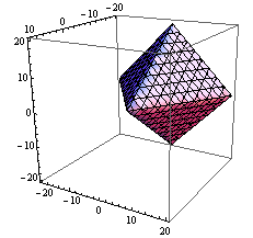
Figure 7. The shape of $C_{1}(0)$ in the case $d=3$.

We introduce the cone with vertex $n\in\Omega_{int}$ by

(8.9) $$C_{1}(n)=\Big{\{}m\in\Omega_{int}\ ;\ \sum_{k\not=1}|m_{k}-n_{k}|\leq-(m_{1}-n_{1})\Big{\}}.$$

If $\widehat{u}$ satisfies the equation (8.8), we have

(8.10) $$\widehat{u}(n)=\sum_{m\in C_{1}(n)\setminus\{n\}}c_{m}\widehat{u}(m)$$

for some constants $c_{m}$. In particular, if $\widehat{u}(m)=0$ for all $m\in C_{1}(n)\setminus\{n\}$, we see that $\widehat{u}(n)=0$ from (8.10) (See also Figure 7).

Let $\Pi(p)$ be the rectangular domain defined by

(8.11) $$\Pi(p)=\big{\{}(n_{1},\cdots,n_{d})\in\Omega_{int}\,;\,n_{1}+n_{d}=p,\ 1\leq n_{i}\leq M\ (2\leq i\leq d-1)\big{\}},$$

where $M$ is from (8.7), and for $r^{\prime}=(r_{2},\cdots,r_{d-1})\in[1,M]^{d-2}$, we consider its section

(8.12) $$\Pi(p;r^{\prime})=\big{\{}(n_{1},n^{\prime},n_{d})\in\Pi(p)\,;\,n^{\prime}=r^{\prime}\big{\}}.$$

For $d=3$, see Figure 8.

Lemma 8.5.

Assume $M+1<p\leq 2M$, and take a point $(p-M-1,r^{\prime},M+1)\in\Pi(p;r^{\prime})$. Let $\widehat{u}$ be the solution of (8.8) with Dirichlet boundary data $\widehat{f}$ such that

$$\left\{\begin{split}&\widehat{f}(p-M-1,r^{\prime},M+1)=1,\\ &\widehat{f}=0\quad\text{on}\quad\partial\Omega_{int}\setminus\big{(}\partial\Omega_{1}^{+}\cup\{(p-M-1,r^{\prime},M+1)\}\big{)},\end{split}\right.$$

and Neumann data $\widehat{g}=0$ on $\partial\Omega_{1}^{-}$. Then we have

(8.13) $$\left\{\begin{split}&\widehat{u}(n)=0\quad\text{if}\quad n_{1}+n_{d}<p,\\ &\widehat{u}(n)=0\quad\text{if}\quad n_{1}+n_{d}=p,\ n^{\prime}\neq r^{\prime},\end{split}\right.$$

(8.14) $$\widehat{u}(p-M-1+i,r^{\prime},M+1-i)=(-1)^{i}\quad\text{for}\quad p-M-1+i\leq M+1.$$

If $p=M+1$, taking the Dirichlet data $\widehat{f}$ such that

$$\left\{\begin{split}&\widehat{f}(0,r^{\prime},M)=1,\\ &\widehat{f}=0\quad\text{on}\quad\partial\Omega_{int}\setminus\big{(}\partial\Omega_{1}^{+}\cup\{(0,r^{\prime},M)\}\big{)},\end{split}\right.$$

we have the same assertion.

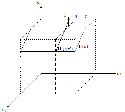
Figure 8. Situation of Lemma 8.5.

Proof. We put $m=(p-M-1,r^{\prime},M+1)$. First we show that $m\not\in C_{1}(n)$, if $n_{1}+n_{d}<p$. In fact,

$$-(m_{1}-n_{1})=n_{1}-(p-M-1)<p-n_{d}-(p-M-1)=M+1-n_{d},$$

and on the other hand,

$$\sum_{k\neq 1}|m_{k}-n_{k}|\geq|m_{d}-n_{d}|=M+1-n_{d}.$$

Then, in view of the condition for $\widehat{f}$, the Neumann data $\partial_{\nu}\widehat{u}|_{\partial\Omega_{1}^{-}}=0$ and (8.10), we have $\widehat{u}(n)=0$ if $n_{1}+n_{d}<p$.

Assume that $n_{1}+n_{d}=p$ and $n^{\prime}\neq r^{\prime}$.

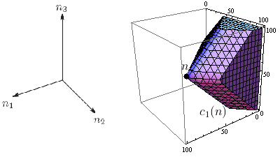
Figure 9. Extension of the solution for the case (8.13).

(See Figure 9.) Then

$$-(m_{1}-n_{1})=M+1-n_{d}.$$

On the other hand, since $n^{\prime}\neq r^{\prime}$, we see that

$$\sum_{k\not=1}|m_{k}-n_{k}|>|m_{d}-n_{d}|=M+1-n_{d}.$$

They imply $m\not\in C_{1}(n)$, hence $\widehat{u}(n)=0$ as above.

Let us prove (8.14). Using the equation

$$((-\Delta_{disc}+\widehat{V})\widehat{u})(p-M-1,r^{\prime},M)=0,$$

and the fact that

$$\widehat{u}=0\quad{\rm for}\quad n_{1}+n_{d}<p,\quad\widehat{u}(p-M-1,r^{\prime},M+1)=1,$$

we have $\widehat{u}(p-M,r^{\prime},M)=-1$. Here we do not use the value of the potential $\widehat{V}(p-M,r^{\prime},M)$. (See Figure 10.)

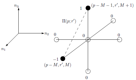
Figure 10. Extension of the solution for the case (8.14).

Repeating this procedure, we see $\widehat{u}(p-M-1+i,r^{\prime},M+1-i)=(-1)^{i}$ inductively. ∎

Now we show the reconstruction procedure.

1st step. We construct the boundary data $\widehat{f}$ such that

$$\left\{\begin{split}&\widehat{f}(M-1,r^{\prime},M+1)=1,\\ &\widehat{f}=0\quad\text{on}\quad\partial\Omega_{int}\setminus\big{(}\partial\Omega_{1}^{+}\cup\{(M-1,r^{\prime},M+1)\}\big{)},\\ &{\bf\Lambda_{\widehat{V}}}\widehat{f}=0\quad\text{on}\quad\partial\Omega_{1}^{-},\end{split}\right.$$

by Corollary 8.4. Then the solution $\widehat{u}$ of (8.1) and (8.4) satisfies the assumption of Lemma 8.5. By virtue of Lemma 8.8, we have

$$\widehat{u}(n)=\left\{\begin{array}[]{cl}-1&(n=(M,r^{\prime},M)),\\ 0&(\text{other}\ n\in\,\stackrel{{\scriptstyle\circ}}{{\Omega}}_{int}).\end{array}\right.$$

Then, using the equality

$$((-\Delta_{disc}+\widehat{V})\widehat{u})(M,r^{\prime},M)=0$$

and the boundary value $\widehat{f}(M+1,r^{\prime},M)$, we can compute the value $\widehat{V}(M,r^{\prime},M)$. Applying this procedure for all $r^{\prime}$, we recover $\widehat{V}$ on all vertices $(n_{1},r^{\prime},n_{d})$ such that $n_{1}+n_{d}=2M$.

2nd step. Assume that we have recovered $\widehat{V}$ on vertices such that $n_{1}+n_{d}>p$ for $M+1<p\leq 2M$. We construct the boundary data $\widehat{f}$ such that

$$\left\{\begin{split}&\widehat{f}(p-M-1,r^{\prime},M+1)=1,\\ &\widehat{f}=0\quad\text{on}\quad\partial\Omega_{int}\setminus\big{(}\partial\Omega_{1}^{+}\cup\{(p-M-1,r^{\prime},M+1)\}\big{)},\\ &{\bf\Lambda_{\widehat{V}}}\widehat{f}=0\quad\text{on}\quad\partial\Omega_{1}^{-}.\end{split}\right.$$

By the same argument as in Step 1, the solution $\widehat{u}$ of (8.1) and (8.4) satisfies (8.13), (8.14). Since we have already recovered $\widehat{V}$ on $n_{1}+n_{d}>p$, we can compute $\widehat{u}(n)$ on $n_{1}+n_{d}>p$ using the equation $(-\Delta_{disc}+\widehat{V})\widehat{u}=0$ and the boundary data $\widehat{f}$. Hence, using the equality

$$((-\Delta_{disc}+\widehat{V})\widehat{u})(p-M-1+i,r^{\prime},M+1-i))=0,$$

and the fact that $\widehat{u}(p-M-1+i,r^{\prime},M+1-i)=(-1)^{i}$, we can compute $\widehat{V}(p-M-1+i,r^{\prime},M+1-i)$ for every $i$. Applying this procedure for all $r^{\prime}$, we recover $\widehat{V}$ on all vertices $(n_{1},r^{\prime},n_{d})$ such that $n_{1}+n_{d}=p$ with $M+1<p\leq 2M$.

3rd step. For $p=M+1$, we construct the boundary data $\widehat{f}$ such that

$$\left\{\begin{split}&\widehat{f}(0,r^{\prime},M)=1,\\ &\widehat{f}=0\quad\text{on}\quad\partial\Omega_{int}\setminus\big{(}\partial\Omega_{1}^{+}\cup\{(0,r^{\prime},M)\}\big{)},\\ &{\bf\Lambda_{\widehat{V}}}\widehat{f}=0\quad\text{on}\quad\partial\Omega_{1}^{-}.\end{split}\right.$$

By the same argument as in Step 1, the solution $\widehat{u}$ of (8.1) and (8.4) satisfies

$$\widehat{u}(n)=\left\{\begin{array}[]{cl}(-1)^{i-1}&(n=(i,r^{\prime},M+1-i)),\\ 0&(n_{1}+n_{d}<p\ \ {\rm or}\ \ n_{1}+n_{d}=p,\ n^{\prime}\neq r^{\prime}).\end{array}\right.$$

Then we can compute $\widehat{V}(i,r^{\prime},M+1-i)$ for every $i$ as above.

4th step. In the case $n_{1}+n_{d}<M+1$, we have only to rotate the whole domain.

We have thus completed the proof of Theorem 1.1.

References

- [1] S. Agmon and L. Hörmander, Asymptotic properties of solutions of differential equations with simple characteristics, J. d’Anal. Math., 30 (1976), 1-38.
- [2] A. Bukhgeim, Recovering the potential from Cauchy data in two dimensions, J. Inverse Ill-Posed Probl., 16 (2008), 19-34.
- [3] E. Curtis and J. Morrow, The Dirichlet to Neumann map for a resistor network, SIAM J. Appl. Math., 51 (1991), 1011-1029.
- [4] E. Curtis, E. Mooers and J. Morrow, Finding the conductors in circular networks from boundary measurements, RAIRO Modél. Math. Anal. Numél., 28 (1994), 781-814.
- [5] J. Dodziuk, Difference equations, isoperimetric inequality and transience of certain random walks, Trans. Amer. Math. Soc., 284 (1984), 787-794.
- [6] M. S. Eskina, The direct and the inverse scattering problem for a partial difference equation, Soviet Math. Doklady, 7 (1966), 193-197.
- [7] O. Y. Imanouilov, G. Uhlmann and M. Yamamoto, The Calderón problem with partial Cauchy data in two dimensions, J. Amer. Math. Soc. 23 (2010), 655-691.
- [8] V. Isakov and A. Nachman, Global uniqueness for a two-dimensional semilinear elliptic inverse problem, Trans. Amer. Math. Soc., 347 (1995), 3375-3390.
- [9] H. Isozaki, Inverse spectral theory, in Topics In The Theory of Schrödinger Operators, eds. H. Araki, H. Ezawa, World Scientific (2003), pp. 93-143.
- [10] H. Isozaki and E. Korotyaev, Inverse problems, trace formulae for discrete Schrödinger operators, Ann. Henri Poincaré, 13 (2012), 751-788.
- [11] H. Isozaki and H. Morioka, A Rellich type theorem for discrete Schrödinger operators, preprint (2012).
- [12] G. M. Khenkin and R. G. Novikov, The -equation in the multi-dimensional inverse scattering problem, Russian Math. Surveys 42 (1987), 109-180.
- [13] W. Littman, Fourier transforms of surface-carried measures and differentiablity of surface averages, Bull, Amer. Math. Soc. 69 (1963), 766-770.
- [14] M. Matsumura, Comportement des solutions de quelques problèmes mixtes pour certains systèmes huperboliques symétriques à coefficients constants, Publ. RIMS, Kyoto Univ. Ser. A 4 (1968), 309-359.
- [15] A. Nachman, Reconstruction from boundary measurements, Ann. of Math. 128 (1988), 531-576.
- [16] A. Nachman, Global uniqueness for a two-dimensional inverse boundary value problem, Ann. Math. 143 (1996), 71-96.
- [17] R. Oberlin, Discrete inverse problems for Schrödinger and resistor networks, Research archive of Research Experiences for Undergraduates program at Univ. of Washington, (2000). http://www.math.washington.edu/~reu/papers/2000/oberlin/oberlin_schrodinger.pdf Accessed 5 July 2012.
- [18] F. Rellich, Über das asymptotische Verhalten der Lösungen von in unendlichen Gebieten, Jahresber. Deitch. Math. Verein., 53 (1943), 57-65.
- [19] W. Shaban and B. Vainberg, Radiation conditions for the difference Schrödinger operators, Applicable Analysis, 80 (2001), 525-556.
- [20] J. Sylvester and G. Uhlmann, A global uniqueness theorem for an inverse boundary value problem, Ann. Math. 125 (1987), 153-169.