Chemical Evolution and the Galactic Habitable Zone of M31 (the Andromeda Galaxy)

Abstract

We have computed the Galactic Habitable Zones (GHZs) of the Andromeda galaxy (M31) based on the probability of terrestrial planet formation, which depends on the metallicity ($Z$) of the interstellar medium, and the number of stars formed per unit surface area. The GHZ was therefore obtained from a chemical evolution model (CEM) built to reproduce a metallicity gradient in the galactic disk, [O/H]($r$) $=-0.015\pm 0.003$ dex kpc${}^{-1}\times r$(kpc) $+0.44\pm 0.04$ dex. This gradient is the most probable when intrinsic scatter is present in the observational data. The chemical evolution model predicted a higher star formation history (SFH) in both the halo and disk components of M31 and a less efficient inside-out galactic formation, compared to those of the Milky Way. If we assumed that Earth-like planets form with a probability law that follows the $Z$ distribution shown by stars with detected planets and the SFH predicted by the CEM, the most probable GHZ per $pc^{2}$ is located between 3 and 7 kpc for planets with ages between 6 and 7 Gy, approximately. But the highest number of stars with habitable planets is in a ring located between 12 and 14 kpc with mean age of $\sim$ 7 Gy. 11 % and 6.5 % of the all formed stars in M31 may have planets capable of hosting basic and complex life, respectively.

Calculamos la Zona de Habitabilidad Galáctica (ZHG) de M31 basándonos en la probabilidad de formación de planetas terrestres dependiente de la metalicidad ($Z$) del medio interestelar. La ZHG fue determinada a partir de un modelo de evolución química construido para reproducir un gradiente de metalicidad en el disco galáctico: [O/H]($r$)$=-0.015$ dex kpc${}^{-1}\times r$(kpc)$+0.44$ dex. Suponiendo que los planetas tipo Tierra se forman bajo una ley de probabilidad que sigue la distribución de $Z$ mostrada por las estrellas con planetas, entonces la ZHG más probable se localiza entre 3 y 7 kpc para planetas con edades entre 6 y 7 Ga, aproximadamente, aunque el mayor número de estrellas con planetas habitables se encuentra en un anillo localizado entre 12 y 14 kpc y edad promedio de $\sim$ 7 Ga. El 11 % y 6.5 % de todas las estrellas formadas en M31 podrían albergar vida básica y compleja, respectivamente.

Galactic habitability Chemical evolution Abundance gradients Andromeda galaxy M31

0.1 Introduction

The Galactic Habitable Zone (GHZ) is defined as the region with sufficient abundance of chemical elements to form planetary systems in which Earth-like planets could be found and might be capable of sustaining life (Gonzalez et al. 2001, Lineweaver 2001). An Earth-like planet is a rocky planet characterized in general terms by the presence of water and an atmosphere (Segura & Kaltenegger 2009).

GHZ research has focused mainly on our galaxy, the Milky Way (MW) (Gonzalez et al. 2001, Lineweaver et al. 2004, Prantzos 2008, Gowanlock et al. 2011). Gonzalez et al. were the first to propose the concept of a GHZ, which is a ring located in the thin disk that migrates outwards with time, due to their most important assumption is that terrestrial planet form with metallicities higher than 1/2 of the solar value ($Z_{\odot}$). Lineweaver et al. (2004) later proposed that the Milky Way’s GHZ is a ring located in the Galactic disk within a radius interval of 7 to 9 kpc from the center of the MW, and that the area of the ring increases with the age of the Galaxy, because they consider a $Z$ distribution, for forming terrestrial planets, that peaks at $\sim 0.8Z_{\odot}$; the presence of a host star; and the absence of nearby supernovae (SN) harmful to life. On the other hand, Prantzos concluded that the current GHZ covers practically the entire MW disk, due to he assumes a $Z$ probability, to form Earth-like planets, almost equal for $Z>0.1Z_{\odot}$. These studies confirmed that the Solar System is located within the GHZ since the Sun is found at 8 kpc from the center of the Galaxy. Nevertheless, a star with an Earth-like planet capable of sustaining life is more likely to be found in inner rings of the Galactic disk, between 2 and 4 kpc, owing to the high stellar surface density that is present in the inner disk of our galaxy (Prantzos 2008, Gowanlock et al. 2011).

The GHZ has recently been computed for two elliptical galaxies (Suthar & McKay 2012). Imposing only metallicity restrictions for planet formation, these authors found that both elliptical galaxies could sustain broad GHZs.

Here, we extend MW studies to the disk of the most massive galaxy in the Local Group: the Andromeda galaxy (M31). M31 is a type SAb spiral galaxy, whose visible mass is $\sim$1.2 times larger than that of the MW, and M31 is at a distance of 783 $\pm$ 30 kpc (Holland 1998).

The GHZ depends mainly on the abundance of chemical elements heavier than He (metallicity, $Z$), since $Z$ leads to planetary formation. Moreover, the GHZ also depends on the occurrence of strong radiation events that can sterilize a planet. Melott & Thomas (2011) study many kinds of astrophysical radiations lethal to life, as electromagnetic radiation (e.g. X rays), high-energy protons or cosmic rays from stars (included the Sun), SN, and gamma-ray bursts (GRB). According to them, the SN and GRB could be the dominant cause of extinctions. Since most of the SN and GRB are originated during the last stages of massive stars, the rate of high-mass stars is useful to estimate the galactic zones where life on planets is annihilated by astrophysical events. In this paper, we excluded the bulge of Andromeda from the GHZ, despite its having a high enough abundance of chemical elements to form planets (Sarajedini & Jablonka 2005). The bulge, located between 0 and 3 kpc from de galactic center, might not provide a stable habitat for life, due to its high supernovae rate at early times, which could sterilize planets, and the proximity of stars that can destabilize the orbits of the planets (Jiménez-Torres et al. 2011).

Throughout this paper the terms ”evolved life” and ”complex life” are synonymous. These terms refer to a type of life similar to that of the human beings, since they are able to develop advanced technologies.

In this study, we present a chemical evolution model (CEM) for the halo and disk components that predicts the temporal behavior of the space distribution of $Z$ and SN occurrence in M31, built on precise observational constraints (Sec. 2). Based on a set of biogenic, astrophysical, and geophysical restrictions, the CEM results lead to the determination of the GHZ (Sec. 3). We discuss the implication of the chemical evolution model and the GHZ condition on the location, size, and age of the Galactic Habitable Zone (Sec. 4). Finally, we present our conclusions of the present study (Sec. 5).

0.2 CHEMICAL EVOLUTION MODEL, CEM

Chemical evolution models study the changes, in space and time, of: a) the chemical abundances present in the interstellar medium (ISM), b) the gas mass, and c) the total baryonic mass of galaxies and intergalactic medium. These studies have a considerable number of free parameters and observational constraints allow us to estimate some of them. If the number of observational constraints is high and the observational data are precise, a more solid model could be proposed and therefore a better estimate of the GHZ can be obtained. In consequence, before building the CEM, we collected and determined a reliable data set of observational constraints.

0.2.1 Observational constraints

The present CEM was built to reproduce M31’s three main observational constraints of the galactic disk: the radial distributions of the total baryonic mass, the gas mass, and the oxygen abundance. Since the data come from several authors, who have adopted different distances, the data used in this work were corrected according to our adopted distance of 783 kpc for M31 (Holland, 1998).

Radial distribution of the total mass surface density in the disk, $\Sigma_{T}(r)$

The luminosity profile is produced by the stellar and ionized gaseous components of the galaxies. In evolved spiral galaxies, such as M31, the current luminosity is mostly due to the stellar component. Because the luminosity profiles of such galaxies follow an exponential behavior with respect to galactocentric distance ($r$), we associated that profile to the radial distribution of total mass surface density, $\Sigma_{T}(r)=\Sigma_{0}exp(-r/r_{d})$ where $r_{d}=5.5$ kpc (Renda et al. 2005). The value for $\Sigma_{0}$ is 548.2 M${}_{\odot}pc^{-2}$ and was obtained by the integration of $\Sigma_{T}(r)$ over the disk’s surface in order to reproduce the total mass disk of M31, which is $7.2\times 10^{10}$ M_⊙ (Widrow, Perrett & Suyu 2003).

Radial distribution of oxygen abundance, [O/H]($r$)

The data were taken from the compilation of M31’s ionized hydrogen (HII) region spectra by Blair et al. (1982) and Galarza et al. (1999). From the total region sample, we rejected those with uncertain measurements of [OII], [OIII], and [NII] lines. Taking into account these prescriptions, the final number of HII regions of our sample is equal to 83. Once we selected our sample, we employed the R₂₃ bi-evaluated method from Pagel et al. (1979), which links the intensity of strong [OII] and [OIII] emission lines with [O/H], to compute the abundances.

The disadvantage of this method is that it is double-valued with respect to metallicity. In fact, at low oxygen abundances ([O/H] $\leq-0.66$) the R₂₃ index decreases with the abundance, while for high oxygen abundances ([O/H] $\geq-0.41$) the metals cooling efficiency makes R₂₃ drop with rising abundance. In order to break the R₂₃ method’s degeneracy, we used [NII]/[OII] line ratios, which are not sensitive to the ionization parameter and are a strong function of O/H above log([NII]/[OII]) $\geq$ 1.2 (Kewley & Dopita, 2002).

To obtain an estimation of the uncertainties in the abundances, we have propagated the error in the line fluxes and added quadratically the accuracy of each method, which is between $\pm$0.1-0.2 dex. It is worth mentioning that the oxygen abundances derived in this study correspond to the composition of the ionized gas phase of the interstellar medium, without taking into account oxygen depletion in dust grains.

In this study, we express the chemical abundances as a function of the galactocentric distance ($r$), related to the Sun as: [O/H]($r$) = log(O/H)($r$) $-$ log(O/H)_⊙, where (O/H) represents the ratio of the abundance by number of oxygen and of hydrogen, and (O/H)_⊙ is this ratio in the Sun, which has a value of $-3.34$ dex (Grevesse, Asplund & Sauval 2007). Moreover, the radial abundance gradient is expressed by the slope and y-intercept value of a linear relationship that fits the trend of empirical abundances as a function of r.

The Galactocentric distances of the objects have been derived taking into account the Galactocentric distances derived by Blair et al. (1982) and Galarza et al. (1999), recomputed for an inclination angle, $i=77\,^{\circ}$, and adopting the distance to M31 from Holland (1998): 783 $\pm$ 30 kpc.

Figure 1: Gradients obtained using different calibration methods. Empirical methods: Pilyugin (2001) and Pilyugin & Thuan (2005). Theoretical methods: McGaugh (1991), Kewley & Dopita (2002), Kobulnicky & Kewley (2004), and Zaritsky et al. (1994). The broad line shows the most probable gradient, computed applying the method of Akritas & Bershady (1996) (see section 2.1.2). This gradient should be reproduced by the chemical evolution model. Note that the theoretical calibration methods give very similar gradients.

In Figure 1, we compile the radial [O/H] gradients obtained from the different empirical and theoretical calibrations. It is clear that all the theoretical methods give very similar results in contrast to the empirical methods, which have much lower y-intercept values even though they keep similar slopes.

Additionally, we tested the effect of the presence of intrinsic scatter in the data in a similar manner to Rosolowsky & Simon’s (2008) method for the gradient of M33 (the third spiral galaxy of the Local Group). Following these authors’ procedure, we applied the method of Akritas & Bershady (1996) to compute the gradients in the presence of an intrinsic scatter. We constructed histograms for each calibration taking into account samples of ten HII regions drawn randomly and we obtained the distributions shown in Figure 2. The final adopted gradient is the weighted average of the four theoretical calibrations we have considered. Hence, the adopted slope is $-0.015\pm 0.003$ dex kpc^-1 and the y-intercept value of [O/H] at the center of M31 is $0.44\pm 0.04$ dex. Finally, we adopted two gradients with which to work: at first, the gradient obtained as the most probable value using the method of Akritas & Bershady (1996) ([O/H]($r$) = $-$0.015 $\pm$ 0.003 dex kpc${}^{-1}\times$ r(kpc) + 0.44 $\pm$ 0.04 dex), which we considered to be representative of the gradients obtained by using photoionization model calibrations. On the other hand, we tried to explore the chemical evolution of M31 by adopting the gradient given by Pilyugin’s (2001) empirical calibration, [O/H]($r$) = $-$0.014 $\pm$ 0.004 dex kpc${}^{-1}\times$ r(kpc) + 0.02 $\pm$ 0.05 dex), a gradient with similar slope but with a y-intercept value 0.42 dex lower compared to the most probable gradient obtained from theoretical calibrations. We also tested the gradient given by Pilyugin & Thuan’s (2005) empirical calibration, which gives a slope 0.006 dex kpc^-1 flatter than all the other calibrations with an intermediate y-intercept value (see section 4.1 for a more detailed discussion).

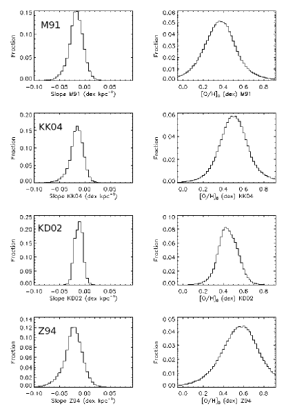
Figure 2: Distribution of the slope (left) and y-intercept (right) of the O/H gradients obtained from the four theoretical calibrations considered in this work: McGaugh (1991) (M91), Kobulnicky & Kewley (2004) (KK04), Kewley & Dopita (2002) (KD02) and Zaritsky et al. (1994) (Z94). The distributions are for samples of ten HII regions drawn randomly from the total sample (see text). See figure 5 of Rosolowsky & Simon (2008) for a similar diagram of M33.

Radial distribution of the gas mass surface density, $\Sigma_{gas}(r)$

$\Sigma_{gas}(r)$ represents all gaseous stages which contain hydrogen, helium, and the rest of the chemical elements, i.e. $\Sigma_{gas}(r)=\Sigma_{H}+\Sigma_{He}+\Sigma_{Z}$.

E. M. Berkhuijsen (2008, private communication), based on Nieten et al. (2006), kindly provided us with the updated atomic and molecular surface density of hydrogen for the northern and southern halves of the disk of M31. We averaged out these data to obtain $\Sigma_{H}$. Taking into account the He and O enrichment by Carigi & Peimbert (2008) ($He$ = 0.25 + 3.3 $\times\ O$, where $He$ and $O$ are abundances by mass), the [O/H] gradient shown in the previous subsection, and scaling $O$ and $Z$ to solar values, we computed $\Sigma_{He}$ and $\Sigma_{Z}$. As additional $\Sigma_{H}$ data, we used the compilation of Renda et al. (2005), which was corrected following the previously described procedure.

In Figure 3a we show both sets of corrected data which we used as $\Sigma_{gas}(r)$ constraints on our chemical evolution model.

0.2.2 Model’s assumptions

In the present article, we built a dual-infall model in an inside-out formation framework (i.e., the galaxy is formed more efficiently in the inner regions than at the periphery), similar to the model used by Renda et al. (2005), Hughes et al. (2008), and Carigi & Peimbert (2011) based on the following assumptions:

1. The halo and the disk are artificially projected onto a two dimensional disk with azimuthal symmetry; therefore, all functions depend only on the galactocentric distance ($r$) and time ($t$).

2. M31 was formed by a dual-infall, $d\Sigma_{T}(r,t)/dt$, of primordial material ($H=0.75$ and $He=0.25$, which are the abundances by mass of hydrogen and helium, respectively) given by the following expression:

   $d\Sigma_{T}(r,t)/dt=a_{h}(r)e^{-t/\tau_{h}}+a_{d}(r)e^{-(t-1{\rm Gy})/\tau_{d}}$.

   The first term represents the halo formation during the first gigayear (Gy), $a_{h}(r)$ was obtained considering the halo’s present-day total surface density profile as $6M_{\odot}{\rm pc}^{2}/(1+(r/8{\rm kpc})^{2})$ and $\tau_{h}=0.1$ Gy according to Renda et al. (2005).

   The second term represents the disk formation from 1 Gy until $t=13$ Gy (current time), where $a_{d}(r)$ was obtained from $\Sigma_{T}(r)$ (see section 2.1.1), $\tau_{d}$ = 0.45 (r/kpc) Gy, which represents the inside-out scenario and such a value was adopted to reproduce the $\Sigma_{gas}(r)$ along with [O/H]($r$) (see sections 2.1.2 and 2.1.3).

3. The star formation rate (SFR) is the amount of gas which is transformed into stars and was parameterized as the Kennicutt–Schmidt law (Kennicutt, 1998), ${\rm SFR}(r,t)=\nu\Sigma_{gas}^{n}(r,t)$, where $\nu$ is the efficiency of star formation and $n$ is a number between 1 and 2. During the halo phase, we chose $n=1.0$ and we obtained $\nu=0.50$ Gy^-1 in order to reproduce the maximum average of metallicity shown by the halo stellar population, log($Z/Z_{\odot})=-0.5$ dex (Koch et al. 2008) ($Z_{\odot}=0.012$ from Grevesse, Asplund & Sauval, 2007). For the disk phase, we chose $n=1.45$, a typical value for the disk of spiral galaxies (Fuchs, Jahrei$\beta$ & Flynn 2009), and we obtained $\nu=0.23$ Gy^-1 (M${}_{\odot}/{\rm pc}^{2})^{-0.45}$ in order to reproduce $\Sigma_{gas}(r)$ along with [O/H]($r$) restrictions at the present time.

4. The initial mass function (IMF) is the mass distribution of the stars formed. We considered the IMF of Kroupa et al. (1993), between a stellar mass interval of 0.1 to 80 M_⊙, since the chemical evolution models that assume this IMF successfully reproduce the chemical properties of the MW’s halo–disk (Carigi et al. 2005) .

5. We adopted the instantaneous recycle approximation, which assumes that stars whose initial mass is higher than 1 M_⊙ die instantly after being created and the chemical elements they produce are ejected into the interstellar medium. This approximation is good for the elements produced mainly by massive stars, such as oxygen, since those stars have short lifetimes ($10^{-3}$ to $10^{-2}$ Gy). The stellar mass fraction returned to the ISM by the stellar population and chemical yields are taken from Franco & Carigi (2008).

6. The loss of gas and stars from the galaxy to the intergalactic medium was not considered. All chemical evolution models of spiral galaxies reproduce the observational constraints without assuming material loss from the galactic disk (e.g. Carigi & Peimbert, 2011). Moreover, no substantial amount of gas surrounding either M31 or the MW has been observed.

7. We do not include radial flows of gas or stars.

0.2.3 Results of the Chemical Evolution Model

Based on the previously mentioned assumptions and the proper values of the free parameters chosen in order to reproduce $\Sigma_{T}(r,t)$, $\Sigma_{gas}(r,t)$ and the most probable [O/H] gradient (see section 2.1) at the present time (13 Gy), we obtained the following results:

Radial distribution of the gas mass surface density, $\Sigma_{gas}$

$\Sigma_{gas}$ was solved numerically for each radius at different times. With the halo and disk prescriptions shown in section 2.2, the predicted $\Sigma_{gas}$ at the present time was found and depicted in Figure 3a along with the data. The maximum of the theoretical $\Sigma_{gas}$ is shifted towards the inner radius compared to the observed values, but the agreement with the central and outer radius is quite good.

We could improve the $\Sigma_{gas}$ agreement for $r<8$ kpc, but the slope of the chemical gradient (the most important constraint in this study) became steeper than the most probable one and it was not precise enough to reproduce the chemistry.

To improve the agreement of $\Sigma_{gas}$ for $r<8$ kpc it may be necessary to assume gas flows through the disk towards the galactic center, as an effect of the Galactic bar (Portinari & Chiosi 2000, Spitoni & Matteucci 2011), which is beyond the scope of this paper. Recently, Spitoni et al. (2013) studied the effects of the radial gas inflows on the O/H gradient of M31. They conclude that the inside-out galactic formation is the most important physical process to create chemical gradients, and the radial flows could be a secondary process. Unfortunately, the effects of the radial gas inflows on the $\Sigma_{gas}$ are not shown.

It is difficult to quantify the implications of the disagreement between observations and model about $\Sigma_{gas}$ at $r<8$kpc, when the other observational constraints are reproduced. Robles-Valdez, Carigi & Peimbert (2013) have found a much better agreement from a more complex chemical evolution model for M31, assuming the lifetimes of each formed star, a more efficient inside-out scenario and $r$-dependent $\nu$ (Tabatabaei & Berkhuijsen 2010, Ford et al. 2013).

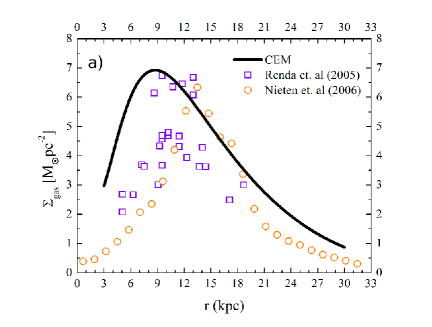
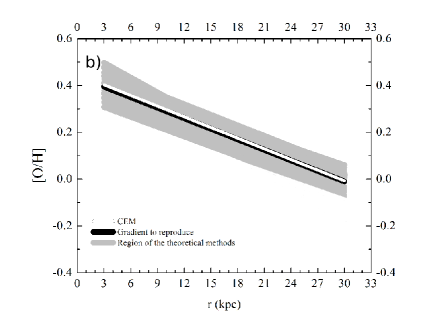
Figure 3: Results of the chemical evolution model (CEM) at the present-time compared to the observational data. a) Radial distribution of the gas mass surface density (see section 2.1.3). b) [O/H] gradient. The white line is the predicted gradient; the black line represents the most probable gradient and the shaded area compiles the gradients obtained by the theoretical methods (see section 2.1.2).

Chemical abundances

The CEM was built to mainly reproduce the O/H gradient determined in this study. That gradient allowed us to obtain a reliable chemical history for M31, where the GHZ will be supported.

In Figure 3b we present the [O/H] gradient predicted by the model at the present time (13 Gy) compared with the observational constraints for M31. The gradients obtained by the theoretical methods were enclosed in the shaded area of the figure, and the adopted gradient, [O/H] = $-$0.015 dex kpc${}^{-1}\times$ r (kpc) + 0.44 dex, was also included in the figure as a broad white line. The gradient obtained from the CEM, [O/H] = $-$0.015 dex kpc${}^{-1}\times$ r(kpc) + 0.45 dex, represented by a solid black line in the figure, is in perfect agreement with the observed value, ensuring the predicted metallicity history.

As previously described, oxygen is the most abundant elemental component of $Z$; a chemical evolution model built to reproduce the [O/H] gradient therefore allows an adequate approximation of the evolution of the heavy elements, represented by $Z$.

Since the GHZ depends mainly on metallicity, we are interested in the evolution of the metal radial distribution; hence, in Figure 4a we show the behavior of log($Z/Z_{\odot}$) with respect to galactocentric distances at different times. It is not surprising that the current gradient of log($Z/Z_{\odot}$), log($Z/Z_{\odot}$) $=-0.015$ dex kpc${}^{-1}\times$ r (kpc) + 0.41 dex, is similar to the [O/H] gradient obtained by the CEM, [O/H] = $-$0.015 dex kpc${}^{-1}\times$ r (kpc) + 0.45 dex, confirming that oxygen is the most abundant heavy element and behaves as $Z$.

From Figure 4a, we notice that the gradient flattens from 3 to 13 Gy, due to the inside-out scenario: at the beginning of the evolution the infall was relevant in the central regions compared to the outer parts, producing higher $\Sigma_{gas}$ and SFR, rapidly increasing the oxygen abundance in the inner regions; then the infall, and therefore the SFR, dropped, causing a lower increase in the oxygen abundance. In contrast, at the final stages of the evolution, the infall became important in the outer regions compared to the inner regions, thus $\Sigma_{gas}$ increased and SFR became more efficient, producing a higher increase in the O abundance in outer regions and, consequently, the gradient became flatter.

The positive slope of the $Z$ gradient at 1 Gy is quite remarkable. This opposite slope behavior is due to the enormous amount of primordial material, from the intergalactic medium, that fell into the inner parts at the beginning of the disk formation, causing gas dilution and a consequent decrease in the O/H values.

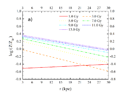
Figure 4: Evolution of radial distributions at 1, 3, 5, 7, 9, 11, and 13 Gy. a) Metallicity relative to the solar value, log($Z/Z_{\odot}$) ($Z_{\odot}=0.012$, Grevesse et al. 2007). b) Star formation rate, SFR. The horizontal line represents the average value of the SFR that the solar neighborhood has undergone during the Sun’s lifetime. (Carigi & Peimbert 2008).

Supernova rate

As we have mentioned, the occurrence of SN is important in the calculation of the GHZ because a high SN rate may deplete the ozone layer in a planetary atmosphere and, thereby, life. Since our CEMs is built using the instantaneous recycle approximation, we cannot estimate the SNIa and consequently, they are not included in the SN rate. That is a model limitation, particularly at high galactic times, because the time-delay of a SNIa to pollute the gas is between 0.1 Gy and the Hubble time (Maoz et al. 2012). That limitation would be counterbalanced by the low average of SNIa in Sbc/d galaxies, like M31 (SNIa/SNII$=0.17$, Mannucci et al. 2005). From the star formation rate inferred by our chemical evolution model, we obtained the SN rate. It was computed according to $RSN(r,t)=N_{MS}\times{\rm SFR}(r,t)$, where $N_{MS}=0.05M_{\odot}^{-1}$ is the number of type II supernova progenitors per $M_{\odot}$. We assumed that those progenitors are stars more massive than 8 $M_{\odot}$ and therefore $N_{MS}$ was calculated by integrating the initial mass function between 8 and 80 $M_{\odot}$.

In Figure 4b, we show the star formation rate as a function of galactocentric distance for the same times shown in Figure 4a. In order to compare with the SFR that occurred in the solar neighborhood during the Sun’s lifetime, we added the average value of the SFR in the solar neighborhood ($r=8$ kpc) over the last 4.5 Gy. That average was obtained from the mean SFR at the solar radius during the last 4.5 Gy, $<$SFR (8 kpc)$>=<$SFR${}_{SV}>=$ 3.8 M_⊙ Gy^-1 pc^-2 (see Fig. 2 by Carigi & Peimbert 2008). Consequently, the 4.5 Gy average SN rate of the solar neighborhood during the Earth’s age is $<RSN_{SV}>=0.2\ Gy^{-1}$ pc^-2.

0.3 Galactic Habitable Zone

The Galactic Habitable Zone (GHZ), is defined as the region with sufficient abundance of chemical elements to form planetary systems in which Earth-like planets could be found and might be capable of sustaining life. Therefore, a minimum metallicity is needed for planetary formation, which would include the formation of a planet with Earth-like characteristics (Gonzalez et al. 2001, Lineweaver 2001), and a CEM provided the evolution of the heavy element distribution (see previous section).

0.3.1 Characteristics and conditions for the GHZ

In this context, it is important to bear in mind the properties and characteristics that an Earth-like planet and its environment need in order to be considered habitable or leading to habitability. In astrobiology, the chemical elements are classified according to the roles they play in the formation of an Earth-like planet and in the origin of life: the major biogenic elements are those that form amino acids and proteins (e.g. H, N, C, O, P, S), the geophysical elements are those that form the crust, mantle, and core (e.g. Si, Mg, Fe) (Hazen et al. 2002).

Astrophysical conditions

The conditions of the environment around an Earth-like planet are the following:

1. Planet formation: The metallicity in the medium where the planet may form (protoplanetary disk) must be such that it allows matter condensation and hence protoplanet formation (Lineweaver 2001). Therefore, Earth-like and Jupiter-like planets may be created. Whether the creation of Jupiter-like planets is beneficial or not is a debatable subject (Horner & Jones 2008, 2009). They may act as a shield against meteoritic impact (Fogg & Nelson 2007, Ward & Brownlee 2000), or might migrate towards the central star of the planetary system, thereby affecting the internal planets, or even destroying them (Lineweaver 2001, Lineweaver et al. 2004). On the other hand, the simulation by Raymond et al. (2006) predicts that Earth-like planets may form from surviving material outside the giant planet’s orbit, often in the habitable zone and with low orbital eccentricities. Most of the planet-harboring stars, detected by several research teams, show a wide range of stellar metallicity, $-0.76\leq{\rm log}(Z/Z_{\odot})\leq+0.56$, and the distribution peaks at log($Z/Z_{\odot})\sim+0.20$ (See Figure 5, lower pannel). Data compilation taken from The Extrasolar Planets Encyclopaedia on March 2013, http://exoplanet.eu/catalog.php). Moreover, based on the same data source, the observed relation between stellar $Z$ abundance and the planet mass presents a wide dispersion. Since that sample includes all types of planets—both Earth-like and Jupiter-like—the stellar $Z-$planet mass relation does not show a clear trend. Recently, Jenkins et al. (2013) have grown the population of low-mass planets around metal-rich stars, increasing the dispersion in the stellar $Z-$planet mass relation. On the other hand, Adibekyan et al. (2012) confirm an overabundance in giant-planet host stars with high $Z$. Therefore, we think that the fraction of detected exoplanets as a function of the metallicity of stars they orbit, represents the necessary $Z$ to form planets that survive to planetary migrations. It should be mentioned that the stellar $Z$ is associated with the planet $Z$ since the planets were created from the same gaseous nebula of the star. Future studies will take into account planet occurrence from Kepler mission (e.g. see Howard et al. 2012).

2. Survival from SN: When a supernova explodes, emits strong radiation that may ionize the planet’s atmosphere, causing the stratospheric-ozone depletion. Then ultraviolet flux from the planet’s host star reaches the surface and oceans, originating damage to genetic material DNA, which could induce mutation or cell death, and consequently the planet sterilization (Gehrels et al., 2003). Since the Earth is the only known planet with life, we assumed it could represent the survival pattern to SN explosions. We have analyzed three possibilities for the planet survival, such that the life on the planet will be annihilated forever if: i) the instantaneous $RSN(r,t)$ is higher than $<RSN_{SV}>$, ii) the average $RSN$, during the entire existence of the planet, is higher than $<RSN_{SV}>$, and iii) the average $RSN$, during the first 4.5 Gy of the planet’s age, is higher than $2\times<RSN_{SV}>$, being $<RSN_{SV}>=0.2\ {\rm Gy}^{-1}{\rm pc}^{-2}$ the time-average of SN rate in the solar neighborhood, during the last 4.5 Gy. In all our RSN computations we have not included SNIa and we could be undervaluing the amount of SN that may sterilize planets, mainly at recent times. We think that this underestimation is compensated for by an overestimation of SNII, due to the instantaneous recycle approximation, and by the low fraction of SNIa ($\sim$ 2 SNIa per 10 SNII) for galaxies like M31 (see section 2.3.3).

Geophysical characteristics

An Earth-like planet is one that has enough biogenic and geophysical elements to sustain and allow the development of life as it is known on Earth (Sleep, Bird & Pope 2012, Bada 2004, Gomez-Caballero & Pantoja-Alor 2003, Hazen et al. 2002, Orgel 1998). In general terms, for a planet to be identified as an Earth-like planet, it has to satisfy the following conditions:

1. Tectonic plates: a crust formed mainly of Si constitutes the tectonic plates. These are necessary since life must have a site to live on with enough resources for survival. The recycling of the tectonic plates keeps the density and the temperature of the planetary atmosphere and the amount of liquid water and carbon needed for life. (Hazen et al. 2002, Lineweaver 2001, Segura & Kaltenegger 2006 ).

2. Water: on the surface of the tectonic plates are found the oceans, formed by H₂O. Since life on Earth is the pattern for life, water is a crucial resource for the emergence and survival of life (McClendon 1999).

3. Atmosphere: the atmosphere of a planet should be dense enough to protect the planet from UV radiation and meteoric impacts, and thin enough to allow the evolution of life on the planet’s surface. The atmospheric composition of the primitive Earth allowed the origin of life and had abundance of CO, CO₂, H₂O, N₂O, and NO₂. Such compounds were crucial to the origin of the present atmosphere on Earth. (Bada 2004, Chyba & Sagan 1991, Maurette et al. 1995, Navarro-González et al. 2001, Sekine et al. 2003).

Since all the geophysical elements are heavier than He, the abundance of these kinds of elements necessary to create an Earth-like planet is both contained and well represented by the distribution of $Z$ given by the chemical evolution model.

Biogenic characteristics

As previously mentioned, the GHZ is based on the pattern of life on Earth; therefore, in order to determine the time of the origin and development of life on Earth several studies were taken into account.

There are several theories of the means and places where life originated on Earth. Some of those theories are based on hydrothermal vents on the seabed, where an interaction between the terrestrial mantle and the ocean exists (Bada 2004, Chang 1982, Gomez-Caballero & Pantoja-Alor 2003, Hazen et al. 2002, McClendon 1999). Other theories have assumed the migration of life from other regions of space to Earth (Maurette et al. 1995, Orgel 1998). There are others explaining the catalytic effect of lightning or metallic meteorites (Chyba & Sagan 1991, Navarro-González et al. 2001, Sekine et al. 2003) in the primitive atmosphere and/or in the seas. Regardless of how life emerged, all theories have agreed on the same biogenic requirements, i.e. C, N, O, P, S. Those biogenic elements are heavier than He and the abundance of these elements is consequently contained and well represented by the distribution of $Z$ given by the CEM.

The earliest evidence we have for life on Earth is about 3.5 Gy ago (the most ancient fossils being cyanobacteria, Kulasooriya 2011, and references therein) or 3.8 Gy (contested carbon isotope evidence, Mojzsis et al. 1996). There is general agreement that life got started 3.7 Gy ago (Ricardo & Szostak 2009). The Earth is $4.6\pm 0.1$ Gy old (Bonanno et al. 2002); therefore, life took around 0.9 Gy to emerge. In consequence, in this study we consider 1.0 Gy as the minimum age of a planet capable of hosting basic life on its surface.

On the other hand, if evolved life is associated with humans, another parameter of life should be taken into account since humans appeared on Earth 2 million years ($2\times 10^{-3}$ Gy) ago (Bada 2004). However, the fact that the times used in our CE study are of the order of gigayears, this $2\times 10^{-3}$ Gy is negligible. Thus, in this study we consider 4.5 Gy as the minimum age of a planet capable of sustaining complex life.

0.3.2 Restrictions for the GHZ

Based on the previously collected information, in order to obtain the evolution of the Galactic Habitable Zone in M31, we chose the following astronomical and biogenic restrictions:

1. Stars might harbor Earth-like planets.

2. Earth-like planets form from gas with specific $Z$-dependent probabilities.

3. Earth-like planets require 1.0 Gy to create basic life (BL).

4. Earth-like planets need 4.5 Gy to evolve complex life (CL).

5. Life on formed planets is annihilated forever by the SN explosions under the following conditions:

   1. the SN rate at any time and at any radius has been higher than the average SN rate in the solar neighborhood ($<RSN_{SV}>$) during the last 4.5 Gy of the Milky Way’s life,

   2. the average $RSN$, during the whole existence of the planet, is higher than $<RSN_{SV}>$, and

   3. the average $RSN$, during the first 4.5 Gy of the planet life, is higher than $2\times<RSN_{SV}>$

Figure 5: Probability of terrestrial planet formation by Lineweaver et al. (2004, upper panel), Prantzos (2008, middle panel) and extrasolar planets (The Extrasolar Planets Encyclopaedia on March 2013, http://exoplanet.eu/catalog.php, lower panel).

Based on the previous assumptions, the probability, $P(r,t)$, to form Earth-like planets, orbiting stars, which survive SN explosions and where basic and complex life may surge is calculated as:

$P_{GHZ}(r,t)=P_{STAR}(r,t)\times P_{Z}(r,t)\times P_{BL}(t)\times P_{CL}(t)\times P_{SN}(r,t)$,

where:

1. $P_{STAR}(r,t)=SFR(r,t)dt$ is the probability of forming new stars, per surface unit ($pc^{2}$), during a delta time.

2. $P_{Z}(r,t)$ is the $Z$-dependent probability of forming terrestrial planets (see Figure 5):

   1. as Lineweaver et al (2004) assume,

   2. as Prantzos (2008) consider, and

   3. identical to the $Z$ distribution shown by extrasolar planets (The Extrasolar Planets Encyclopaedia on March 2013, http://exoplanet.eu/catalog.php).

3. $P_{BL}(t)$ and $P_{CL}(t)$ are the probabilities of the emergence of basic life and the evolution of complex life. We adopt functions with no dispersion (equal to 0.0 or 1.0) because the uncertainties in the evidence for life are similar to the temporal resolution of the chemical evolution model.

4. $P_{SN}(r,t)$ is the probability of survival of supernova explosions. We adopt $P_{SN}(r,t)=1.0$ or $P_{SN}(r,t)=0.0$ if SN rate is lower or higher than the average $RSN$, respectively. This is a good approximation because of the quick decay of $P_{SN}$ (Lineweaver et al. 2004) and the two extreme conditions supported on the pattern of life and considered in this study.

0.3.3 Results of the Galactic Habitable Zone

Our chemical evolution model—explained in section 2—provided the evolution of: metals, star formation rate, and SN rate at different galactocentric distances, which are the data required to compute the Galactic Habitable Zone. We then applied the restrictions listed in the previous sections on the galactic disk of M31 and obtained GHZs. Since most previous studies of the GHZ have focused on the Milky Way (Lineweaver et al. 2004, Prantzos 2008, Gowanlock et al. 2011), we also obtained the GHZ of the Andromeda galaxy using their common restrictions in order to compare the GHZ in both neighboring spiral galaxies using identical galactic habitable conditions.

SN effects on the GHZ

Based on the results of the chemical evolution model, we found the galactic times and regions in the galactic disk where the metallicity satisfies the exoplanet distribution, then we account for the number of formed stars and we apply the condition of SN survival.

Figure 6: Evolution of the Galactic Habitable Zone of M31 assuming the $Z$ distribution shown by exoplanets, three different supernova survival conditions, and two type of life on the exoplanets. Planet are sterilized if: i) the instantaneous SN rate is higher than the time-average SN rate of the solar neighborhood during the Sun’s existence, $<RSN_{SV}>$(upper panels), ii) the average SN rate during the planet’s entire existence is higher than $<RSN_{SV}>$ (middle panels), and iii) the average $RSN$ during the first 4.5 Gy of the planet life is higher than $2\times<RSN_{SV}>$ (lower panels). Planets capable ofsustaining basic life (left panels) or evolved life (right panels). Burgundy area: zone where life may be extinguished by SN explosions. Grey area: zone where planets may not harbor life. Red and violet areas: zones with maximum and minimum probabilities, respectively, to form Earth-like planets orbiting stars. Other colors: intermediate probabilities of the GHZ.

In Figure 6 we show the evolution of the GHZ, per surface unit, assuming these constraints for three SN survival conditions ; i. e. the planet sterilization occurs if: i) the instantaneous SN rate is higher than $<RSN_{SV}>$ (upper panels), ii) the average SN rate during the planet’s entire existence ($<RSN(r,t)>_{planet\ age}$) is higher than $<RSN_{SV}>$ (middle panels), or iii) the average $RSN$ during the first 4.5 Gy of the planet life ($<RSN(r,t)>_{4.5Gy}$) is higher than $2\times<RSN_{SV}>$ (lower panels). Moreover, we imposed the restriction of basic life (1 Gy, left panels) and evolved life (4.5 Gy, right panels).

We mark where and when planets were sterilized (burgundy) and where and when planets may not be capable of hosting basic and complex life (grey). We indicate with differently colors the probability values to form Earth-like planets that orbit stars. The red and violet areas represent the zones with maximum and minimum probabilities.

The GHZs shown in Figure 6 are smaller at high planet ages (equivalent to low evolutionary time) and excludes short galactocentric radii, due to the inside-out formation scenario, upon which the chemical evolution model was built. That model predicts a high star formation rate at inner radii during the first moments of evolution and, consequently, a high SN rate that would have sterilized the planets formed there.

If life has not recovered after $RSN(r,t)=<RSN_{SV}>$, the most likely GHZ is located in the middle galactic disk ($10-18$ kpc). But if life has not recovered when $<RSN(r,t)>_{planet\ age}=<RSN_{SV}>$ the most likely GHZ is located in the very inner galactic disk ($3-5$ kpc).

Since life on Earth has proven to be highly resistant, we think that the GHZ assuming $<RSN(r,t)>_{4.5Gy}=2\times<RSN_{SV}>$ is more reliable. Therefore, based on the lower panels of Figure 6, the most likely GHZ (per surface unit) is located in the inner disk ($3-7$ kpc) with ages between 6 and 7 Gyr. The GHZ with median probabilities evolves from the middle ($\sim 13$ kpc) to the inner disk, from 4.5 Gy to 8.0 Gy age. If we consider only basic life, the younger GHZ evolves away from the inner parts. In either case, the halo component (for evolution times lower than 1 Gy at any $r$) is discarded from the GHZ because of its low $SFR$ and $Z$.

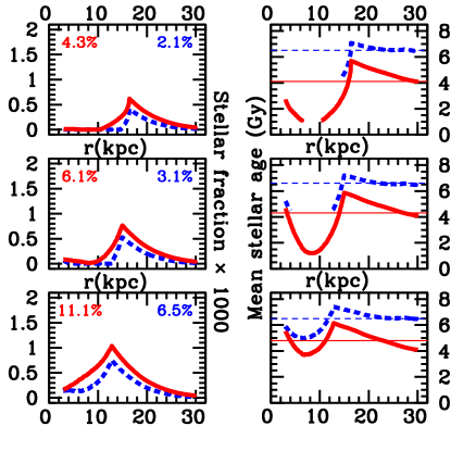
Figure 7: Left panels: $0-13$ Gy integrated fraction of stars harboring terrestrial planets formed according to $Z$ distribution shown by exoplanets and that survive SN explosions: $RSN(r,t)\leq\ <RSN_{SV}>$ (upper panels), $<RSN(r,t)>_{planet\ age}\leq\ <RSN_{SV}>$ (middle panels), and $<RSN(r,t)>_{4.5Gy}\leq 2\times<RSN_{SV}>$ (lower panels). Red-continuous lines: basic life. Blue-dashed lines: complex life. Left and right corners: total percentage of planetary systems capable of sustaining basic life or complex life, respectively, on their Earth-like planets. Right panels: mean age of the stellar fractions shown in the left panels. Thin lines: the average age of the total stars with solid planets that survive SN.

In the left panels of Figure 7, for the same GHZs of Figure 6, we plot the fraction of stars with terrestrial planets that survive SN explosions, taking into account basic and complex life may surge (red-continuous and blue-dashed lines, respectively). That fraction represents the $0-13$ Gy integrated number of those stars formed in a d$r-$width ring centered in each $r$, normalized by the total number of stars formed in the $3-30$ kpc disk. In the left and right corners, we show the total percentage of stars harboring Earth-like planets that survive SN and capable of hosting basic life or evolved life, respectively. Obviously, the percentage with basic life is higher than the percentage with complex life, and both percentages increase with the life’s resistance to the SN harmful effects. It is important to note that the peak in the stellar fractions are not located at the same radius as the GHZs due to the time-integration of the $P_{GHZ}(r,t)$ and the total area of each ring.

In the right panels of Figure 7 we plot the mean age of the stellar fractions shown in the left panels. In the upper and middle windows there are not data for some radii less than 15 kpc, due to all terrestrial planets formed at those $r$ were sterilized by SN.

For $r<13-15$ kpc, the stellar fraction and the mean stellar age decrease with the increase of SN effects. For $r>15$ kpc, the $r$ behavior of the stellar fraction and the mean stellar age are identical between GHZs because the SN effects are null and the $P_{STAR}(r,t)$ and $P_{Z}(r,t)$ are identical. The thin lines represent the average age of the total stars harboring Earth-like planets that survive SN. For complex life and any SN survival conditions, the average stellar age is $\sim 6.5$ Gyr, but for basic life the average age is $4-5$ Gy and increasing with life’s resistance to the SN effects.

$Z$ effects on the GHZ

Four of the five previous studies of the GHZ (Gonzalez et al. 2001, Lineweaver et al. 2004, Prantzos 2008, Gowanlock et al. 2011, Suthar & McKay 2012) have focused on the Milky Way.

Lineweaver et al. (2004), Prantzos (2008) and Gowanlock et al. (2011) have computed the GHZ of the MW assuming specific $Z$ ranges to form Earth-like planets and for SN survival. Since Gowanlock et al. adopted a much wider $Z$ range than that of Lineweaver et al., with probabilities lower and almost $Z$ independent, similar to that by Prantzos, we computed the GHZ of M31 based on the assumptions of Lineweaver et al. and Prantzos, separately (Figure 5, upper and middle panels). Moreover we considered that life is annihilated forever when $<RSN(r,t)>$, during the first 4.5 Gy of the planet, is higher than $2\times<RSN_{SV}>$, SN condition similar to that used by Lineweaver et al. and Prantzos.

Figure 8: Evolution of the Galactic Habitable Zone of M31 assuming that planet sterilization occurs when the average $RSN$ during the first 4.5 Gy of the planet is higher than $2\times<RSN_{SV}>$ and three different $Z$ probability of forming terrestrial planets (see Figure 5) by: i) Lineweaver et al. (2004, upper panels), ii) Prantzos (2008, middle panels), and iii) extrasolar planets (2013, lower panels). Planets capable of hosting basic life (left panels) or evolved life (right panels). Colors as Figure 6.

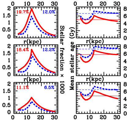
Figure 9: Left panels: $0-13$ Gy integrated fraction of stars harboring terrestrial planets that survive SN explosions and forming according to three different $Z$ probability (see Figure 5): Lineweaver et al. (2004, upper panels), Prantzos (2008, middle panels), and extrasolar planets (2013, lower panels). Lines and percentages as Figure 7.

First, we computed the GHZ of M31 using Lineweaver et al.’s $Z$ distribution: Earth-like planets, that survive the migration of Jupiter-like planets, and formed in regions that fulfill the $Z$ dependent probability shown in Figure 5 (upper panel). That probability peaks at log($Z/Z_{\odot}$) $\sim 0.1$ and is poorly populated at high metallicities, comparing to the extrasolar planets probability.

In Figure 8 (upper panels) we show the M31 GHZ, taking into account the Lineweaver et al.’s $Z$ distribution, and also we impose the basic and complex life conditions. The GHZ maximum is located between 3 and 13 kpc, with ages between 5 and 8 Gy due to that $Z$ probability presents a pronounced maximum between 0.05 and 0.2 dex, being that probability more important than $P_{STAR}$ at that radii and times.

Then, we computed the GHZ adopting the Prantzos’ $Z$ distribution to form terrestrial planets, that survive the migration of gaseous planets: an almost $Z$ independent probability for a wider $Z$ range, $-1.00\leq$ log($Z/Z_{\odot}$) $\leq+0.50$, (Figure 5, middle panel).

In Figure 8 (middle panels) we show the M31 GHZ assuming Prantzos’ $Z$ distribution plus the basic and complex life conditions. The maximum GHZ is located between 3 and 5 kpc, with ages between 6 and 7 Gy, where and when the $SFR$ is high enough to form a huge numbers of stars, but not so high to sterilize their planets. In this case it is possible to find, with medium probability, younger (age $<$4 Gyr) planets located in the inner disk ($r<5$ kpc) and older planets (age $>6$ Gyr) located in the central disk ($12<r<20$ kpc). Since the $P_{Z}$ is almost constant, the GHZ behavior is determined mainly by the $SFR$ and SN events.

For comparison, we present in Figure 8 (lower panels) the GHZ adopting the $Z$ distribution shown by the exoplanets. That probability has a wide peak slightly moved to higher metallicities (Figure 5, lower panel). The maximum GHZ is located between 3 and 5 kpc, with ages between 6 and 7 Gy, due to that $P_{Z}$ peaks at log($Z/Z_{\odot}$) $\sim 0.2$, where the $P_{STAR}$ is important.

In the left panels of Figure 9, for the same GHZs of Figure 8, we plot the $0-13$ Gy integrated fraction of stars with terrestrial planets unsterilized by SN. The numbers at the left and right corners represent the total percentages of those planetary systems capable of sustaining basic life or evolved life, respectively. Both percentages increase with the mean probability of the $Z$ distribution. The width at half maximum of the stellar fractions are located at $9.7<r(kpc)<18$, $10.0<r(kpc)<18$ and $9.0<r(kpc)<18$ for Lineweaver et al. (2004), Prantzos (2008), and exoplanets (2013) distributions, respectively, due to the $P_{Z}/P_{Z}^{max}$ values at high $Z$. For $r<12.5$ kpc and $r>12.5$ the decline rate of the stellar fractions rate reflects the $P_{Z}$ behavior at super solar and subsolar metallicities, respectively. Again, the stellar fractions peak at higher radii than GHZs peak, due to the time-integration of the $P_{GHZ}(r,t)$ and the area of each concentric ring.

In the right panels of Figure 9 we plot the mean age of the stellar radial distribution present in the left panels. The thin lines represent the average age of the total stars harboring Earth-like planets capable of hosting life. For $r>12$ kpc when: i) $P_{Z}$ by Prantzos (2008) is used, the mean stellar ages are higher than those by Lineweaver et al. (2004) and exoplanets (2013) distributions, producing average stellar ages higher by 1 Gy, approximately. That fact is due to that distribution presents a plateau of maximum probability for low $Z$, increasing the number of metal poor and older stars. ii) $P_{Z}$ by exoplanets (2013) distribution is assumed, the mean ages are lower, because that distribution shows low probabilities for low $Z$.

0.4 DISCUSSION

0.4.1 Chemical Evolution model

A chemical evolution model can be computed with three minimum observational constraints at the present time: total baryonic mass, gas mass, and the abundance of one chemical element. In this study we have compiled from the updated literature and well described $\Sigma_{T}(r)$ and $\Sigma_{gas}(r)$ distributions, and we have determined a O/H gradient from H 2 regions. Based on these quite restrictive constraints, we obtained a solid chemical evolution model of the halo and disk of M31.

The chemical evolution model was built to match the most probable O/H gradient, [O/H]($r$) = $-$0.015 dex kpc^-1 $\times$ r(kpc) + 0.44 dex, determined considering the intrinsic scatter and several theoretical calibrations (see section 2.1.2). This gradient is caused by the inside-out scenario: the infall is faster and more abundant in inner regions, producing a more efficient SFR, which increases the O/H abundance of the inner parts faster than that of the outer parts.

In this study, we also explored the gradient determined by empirical calibrations and proposed by Pilyugin (2001) and Pilyugin & Thuan (2005). The gradient obtained through the Pilyugin (2001) calibration presents the same slope, but its y-intercept value is lower by 0.42 dex than that obtained from theoretical calibrations. On the other hand, the gradient obtained by using the Pilyugin & Thuan (2005) calibration, [O/H]($r$) =$-$0.008 dex kpc^-1 $\times$ r(kpc) $-$ 0.23 dex, is 0.007 dex kpc^-1 flatter and the y-intercept value lower by 0.67 dex than that obtained from theoretical calibrations. We were not able to reproduce the Pilyugin gradient without overestimating the $\Sigma_{gas}(r)$ distribution.

Peimbert et al. (2007) suggested that the abundances derived from the R₂₃ empirical calibrations could be underestimated due to the presence of temperature variations in the ionized volume, which leads to the overestimation of the electron temperatures, and that the use of empirical calibrations based on optical recombination line measurements (which are much less affected by temperature variations and give abundances similar to those obtained using theoretical calibrations) could reconcile the R₂₃ theoretical calibrations with empirical ones. This is a well known problem in the astrophysics of photoionized nebulae (see Peimbert et al. 2007 and references therein for more discussion about this topic).

The slope of the O/H gradients we computed are in some way steeper, but are consistent, within the errors, to those derived from supergiants within 12 kpc of the galactic center reported by Trundle et al. (2002), which amounts to $-$0.006$\pm$ 0.020 dex kpc^-1. Venn et al. (2000) had also found that there was no oxygen gradient between 10 kpc and 20 kpc; however, their study was based on abundance determinations for only three A–F supergiants and their results are therefore inconclusive. Our result is also consistent with the canonical M31 gradient derived by Zaritsky et al. (1994) ($-$0.020$\pm$0.007). Very recently, two exhaustive works on the O/H gradient from H 2 regions have been developed: Zurita & Bresolin (2012), from the analysis of 85 H 2 regions, computed an O/H gradient of $-$0.023$\pm$0,002 dex kpc^-1, which is somewhat steeper than ours. Depending on the adopted strong line method, they find a central (y-intercept) [O/H] abundance in the range 0.02$-$0.22, which is 0.22$-$0.42 dex lower than the value we have adopted. On the other hand, Sanders et al. (2012) have developed the most extensive work on the O/H gradient in M31 to date; they computed the O/H gradient using several strong line calibration methods applied to more than a hundred H 2 regions, particularly, applying their prefered strong line method (those of Nagao et al., 2007) to 192 H 2 regions, they find an O/H gradient of $-$0.0195$\pm$0.0055 dex kpc^-1 with a central [O/H]=0.44$\pm$0.07, in excellent agreement with the values computed in this work. However, from direct abundance measurements in 51 planetary nebulae (PNe) they do not find a significant O/H abundance gradient. Finally, Kwitter et al. (2012) have recently computed a radial O/H gradient from PNe data; they derive a gradient of $-$0.011$\pm$0.004 dex kpc^-1, which is consistent, within the errors, with our value derived from H 2 regions. We need additionally to bear in mind that, although the values of the gradient we have obtained are somewhat shallower than typical values for spiral galaxies, recent results seem to confirm that M31 is a barred spiral galaxy (see Beaton et al. 2007, Athanassoula & Beaton 2006 and references therein), which produce shallower gradients than normal spiral galaxies (Friedli et al. 1994).

The $\Sigma_{gas}$ obtained from the chemical evolution model follows a similar pattern to that observed at radii larger than 9 kpc. However, at smaller radii the model predicted more gas than observed. Since $\Sigma_{gas}$, at a fixed galactocentric distance, decreases due to the SFR and increases mainly due to infall, we tried to reproduce at smaller r values the $\Sigma_{gas}$ increasing the SFR, but the slope of the O/H gradient became steeper than the most probable one. In addition, we tried to solve the discrepancy between the model and the observed $\Sigma_{gas}$ at low radii, changing the radial distribution of the infall, but the agreement with the observed $\Sigma_{T}$ was lost. It is possible to reduce $\Sigma_{gas}$ in the inner part by adopting gas inflows to the galactic bar ( Portinari & Chiosi 2000, Spitoni & Matteucci 2011). That assumption will be considered in a future article.

The predicted distribution of the SFR at 13 Gy agrees with the observed one (see data collected by Yin et al. 2009 and Marcon-Uchida et al. 2010) for inner regions, but is in disagreement for outer regions. On the other hand, the agreement between the predicted and observed $\Sigma_{gas}$ is good for the outer regions, but not for inner regions. Since the SFR assumed in this study depends on the gas mass, there is an inconsistency between the observed $\Sigma_{gas}$ and the SFR. Therefore, it is not obvious how to change the two free parameters of our SFR (see section 2.2) to match both the $\Sigma_{gas}$ and the SFR distributions with the observed values. In order to improve the agreement of the obtained $\Sigma_{gas}$ and SFR, we needed to consider different accretion and star formation laws based on more complex physical properties for galactic and star formation.

Renda et al. (2005), Matsson (2008), Yin et al. (2009), and Marcon-Uchida et al. (2010) have computed CEMs for the Andromeda galaxy taking into consideration different assumptions and using diverse codes, but with a common consideration: two-dimensional disk model with negligible height, as our model. That is a model limitation, in particular if we like to study the chemical properties of the thin and thick disks, which is beyond the scope of this paper. If a three dimensional model were implemented, the general properties of the disk would not be so different, because the inside-out nature of disc growth (main assumption in our models) is obtained as a consequence from cosmological hydrodynamical simulations (Brook et al. 2012).

These models were built to reproduce different O/H gradients, which show higher dispersion or error, with O/H differences at a given $r$ value in the 0.4 to 0.7 dex range; consequently, these models are not constrained as well as our model. In particular the agreements of the Marcon-Uchida et al. model are poorer or marginal.

We also made a comparative study of the chemical evolution models and the observational constraints of the Milky Way galaxy with the Andromeda galaxy, and we noticed that:

1. The maximum average of the Fe/H abundances present in the halo stars of M31 corresponds to log($Z/Z_{\odot}$)= $-$0.5, while in the MW it amounts to $-$1.6 (Koch et al. 2008). In order to reproduce the higher $Z$ value in the halo stars of M31, our model requires, in the halo phase, a more efficient infall ($\tau_{h}$ is about 5 times lower) and SFR (two orders of magnitudes higher) than those for the MW model computed with similar assumptions (Carigi et al. 2005, Carigi & Peimbert 2011).

2. The adopted gradient for M31, [O/H]($r$) = $-$0.015 dex kpc^-1 $\times$ r (kpc) + 0.44 dex, is 0.03 dex flatter and 0.06 dex higher in the central value than the O/H gradient of the Milky Way disk determined by Esteban et al. (2005) from optical oxygen recombination lines. In order to reproduce the flatter M31 gradient, our model needed, in the disk phase, a less marked inside-out formation, i.e. slower infall in the inner regions and faster accretion in the outer parts compared to the infall considered in CEMs of the MW. Moreover, to reach the higher O/H values, the model required a more active star formation history than that assumed for the MW disk (Carigi & Peimbert 2011), resulting in a lower $\Sigma_{gas}(r)$ in M31 than in the MW, in agreement with the observed distribution in both galaxies.

0.4.2 Galactic Habitable Zone

The chemical evolution model discussed above provides the evolution and location of the heavy elements of which planets are formed, the stellar surface density, and the rate of neighboring SN that may sterilize life on the planets. The age and the location of potential life-bearing planets inside a galaxy depend on the $Z$ range assumed to form those planets and on the number of stars harboring planets.

Using the $Z$ distribution shown by the exoplanet encyclopaedia (2013) we studied the SN effects on the GHZ per $pc^{2}$ assuming three different permanent planet sterilization conditions: $RSN(r,t)$, $<RSN(r,t)>_{planet\ age}$, and $1/2<RSN(r,t)>_{4.5Gy}$ is higher than $<RSN_{SV}>$ From Figures 6 and 7, we note that SN effects are more important in the inner disk during the first half of the galactic evolution. Moreover, we figure out when life’s resistance to SN danger increases: i) the location of the most probable GHZ per $pc^{2}$ shifts from the central concentric rings ($12<r(kpc)<18$) to the inner rings ($3<r(kpc)<6$), ii) the average stellar age increases, and iii) the total number of star harboring unsterilized planets increases.

The SN condition for extinguishing the life on a planet is the most uncertain restriction, because it is difficult to estimate the resistance of life to SN explosions, which depends on unknown biogenic and astrophysical factors, such as the minimum SN-planet distance that allows life to survive, the type of atmosphere and oceans where life could evolve, and the biological properties of the different types of life, among others factors. Due to life on the Earth has been able to recover massive extinctions, caused by different events, including neighbor SN events, we consider that the double of the average SN rate of the solar neighborhood, since the Earth formed ($<RSN(r,t)>_{4.5Gy}$) is the maximum average that life can withstand on an planet.

Assuming that life disappear forever if $<RSN(r,t)>_{4.5Gy}$ is higher than $2\times<RSN_{SV}>$, we studied the Z effects on the GHZ per $pc^{2}$ considering three different $Z$ probability distribution to form Earth-like planets: Lineweaver et al. (2004), Prantzos (2008), and extrasolar planets (2013). From Figures 8 and 9, we note that Z effects are more important in the inner disk during the second half of the galactic evolution. Moreover, we figure out that when: i) the distribution peaks at higher $Z$, the location of the most probable GHZ per $pc^{2}$ shifts from the inner disk ($3<r(kpc)<12$) to the very inner rings ($3<r(kpc)<5$), ii) the $Z$ distribution is weighted to low $Z$, the average stellar age increases, and iii) the half maximum value of the distribution increases, the total number of star harboring terrestrial planets increases. It is difficult to quantify the role of metallicity in planet formation. At present, theoretical models fail to explain in detail the physical processes in protoplanetary disks and in particular the metallicity effect on the planet mass (rocky like Earth or gaseous like Jupiter). Furthermore, the observational data of detected extrasolar planets do not show a clear trend between the stellar metallicity and the planet mass that orbit around it. Recent Jenkins et al. (2013) have increased the number of low-mass planets around metal-rich stars. However, Adibekyan et al. (2012) confirm an overabundance in giant-planet host stars with high $Z$. Also, it is noticeable that in many detected extrasolar planetary systems, Earth-like and Jupiter-like planets coexist (The Extrasolar Planets Encyclopedia). Moreover, Raymond et al. (2006) have simulated terrestrial planet growth during and after giant planet migration. Observational studies on the circumstellar disk in young stellar clusters of low and solar metallicities suggest that the disk lifetime shortens with decreasing $Z$, thereby reducing the time available for planet formation (Yasui et al. 2010). Based on circumstellar disk models and dust grain properties, Johnson & Li (2012) conclude that the first Earth-like planets likely formed from gas with metallicities $Z>0.1\ Z_{\odot}$.

For these reasons we preferred the $Z$ distribution shown by exoplanet-harboring stars as the metallicity condition for the GHZ instead of undertaking a probability study of planet formation and migration as a function of metallicity, as did Lineweaver (2001), Prantzos (2008), and Gowanlock et al. (2011).

Based on the previous discussion, we deduce that: the most probable GHZ per $pc^{2}$ is located in the galactic disk of M31 between 3 and 7 kpc and ages between 6 and 7 Gy, assuming both basic and complex life (see Figures 6 and 8, lower panel), but the highest amount of stars harboring planets that survive SN is in an annular region of 13 kpc radius and 2 kpc width, with mean ages of 5.8 and 7.0 Gy, for basic and complex life, respectively.

In GHZ studies the galactic formation scenario is crucial for finding the location and number of planetary systems with at least a terrestrial planet, because the galactic formation scenario determines the infall rate, that provides the gas to form stars, when those stars die enrich the ISM with heavy chemical elements, from that metals planets form, and those planets far enough from SN, survive.

Comparison with GHZ of the MW

The GHZs for the MW were obtained by Lineweaver et al. (2004), Prantzos (2008) and Gowanlock et al. (2011) from similar chemical evolution models, built on the inside-out scenario, consequently, the SFR(r,t) and Z(r,t) can be considered equal in all MW GHZs. Therefore the differences among those GHZs are caused by the differences in the assumed probabilities, mainly in the $Z$ distributions to form terrestrial planets. Since one of the scopes of this paper is to find the differences in the habitability of Milky Way and Andromeda galaxies, we computed in section 3.3.2 GHZs for M31, based on the $Z$ probability used by Lineweaver et al. and Prantzos (Gowanlock et al’s distribution is almost constant, as Prantzos’ one).

First, Lineweaver et al. (2004) found that the GHZ of the MW is located in the inner-central Galactic disk, like our GHZ of M31, based on the same $Z$ probability (see Figure 8, upper panel). Their GHZ with probabilities higher than 68%, and complex or basic life, is a wide ring between $r=4$ kpc and 11 kpc, which area corresponds to 26% of the Galactic disk area considered by those authors ($\sim\pi(20^{2}-2.5^{2})kpc^{2}$). In our work, the GHZ with $P_{GHZ}>0.68$ is a ring between 3 and 12 kpc that corresponds to 15% of the galactic disk of M31 ($\sim\pi(30^{2}-3^{2})kpc^{2}$). According to Lineweaver et al. less than 10% of stars formed in MW have a probability higher than 0.68 to harbor terrestrial planet capable of sustaining complex life, but in our GHZ that percentage is 1.6% and corresponds, approximately, to the stellar fraction between 3 and 10 kpc (see Figure 9, upper panel).

Second, Prantzos (2008) found that the GHZ, only for basic life, is located in the inner Galactic disk, like our GHZ of the M31, based on the same $Z$ probability (see Figure 8, middle panel). His GHZ, with probabilities higher than 50% is a ring between $r=2$ kpc and 8 kpc, that corresponds to 17 % of the Galactic disk area considered by him ($\sim\pi(19^{2}-2^{2})kpc^{2}$). In our work, the GHZ with $P_{GHZ}>0.50$ is a ring between 3 and 12 kpc that corresponds to 15% of the M31 galactic disk. Unfortunately, he does not mention the percentage of stars suitable for life, but in our GHZ that percentage is 1.7 % and corresponds to stellar fractions between 0.2 and 0.3 values in the 3-12 kpc range.

Then, Gowanlock et al. (2011) found that the GHZ, only for complex life, is located toward the inner Galaxy. It is not easy to compare their GHZ and ours, because they did more precise and complete computations, assuming, e.g. three dimensional disk, probabilities from SN survival condition based on the planet-SN distance, SNII and SNIa, and tidal locking. If we focus only on the common ingredients ($P_{STAR}$ and $P_{Z}$), we confirm that their $P_{STAR}$ is similar to ours, due to inside-out scenario, but their $P_{Z}$ is similar to Prantzos one, because their probability is almost independent on $Z$. Therefore, if a comparison could be done is with our GHZ that considers the $Z$ probability by Prantzos (2008, see Figure 8, middle panel). The width of the half maximum probability of their GHZ is located between 3 and 8 kpc, that corresponds to 25 % of the Galactic disk area considered by them ($\sim\pi(15^{2}-3^{2})kpc^{2}$), but our percentage is 15 %. According to Gowanlock et al. 1.2 % of all stars formed in MW host a planet suitable for life, but based on Figure 9 (middle panel) our percentage is a factor of 10 larger (12.2 %).

Unfortunately, the comparison of the GHZs between the MW and M31, based on stellar fractions and galactic rings where stars harboring habitable planets are located, was not conclusive. The only property that we could infer is the position of the most likely GHZ, which depends on the $Z$ probability assumed. A more successful comparative study will be obtained when the GHZ of the MW is computed from identical constraints. That comparison will be shown in a future paper and will allow to explore the effect on the GHZ of the intrinsic differences among spiral galaxies.

Throughout this section we have emphasized that the chemical content is one of the most restrictive condition to the GHZ. Furthermore, we have mentioned that the slope of the $Z$ gradient is determined by the efficiency of inside-out scenario, whereas the y-intercept values of the gradient depend on by the amount of accreted gas and the star formation efficiency. Therefore, we stress that the manner in which a galaxy is assembled and its stars formed determine the size and age of the GHZ.

0.5 Conclusions

Based on O/H values of H 2 regions, we obtained current O/H gradients with different empirical and theoretical calibrations. In the presence of intrinsic scatter, we computed the most probable gradient for M31 from theoretical calibrations based on the R₂₃ method and we found that [O/H]($r$) = $-0.015\pm 0.003$dex kpc${}^{-1}\times r(kpc)+0.44\pm 0.04$ dex. The slope of the gradient is 0.03 dex kpc^-1 flatter, and the value at the center of the galaxy is 0.06 dex higher, than those values of the O/H gradient of the Milky Way disk.

The chemical evolution model built to reproduce our O/H gradient of the galactic disk matches the current radial distribution of the gas mass, $\Sigma_{gas}(r)$, for the outer regions quite well, but it fails for the inner ones. On the other hand, the current radial distribution of the star formation rate, SFR($r$), fits for the inner parts, but not for the outer ones. Therefore, in order to improve the agreements, the model would require more complex galactic and star formation histories.

The model cannot reproduce the O/H gradient computed by empirical methods, which is 0.42 dex lower for the central value than the gradient obtained by theoretical methods, unless the other observational constraints are considerably modified.

Based on the chemical evolution model we obtained, for the first time, the Galactic Habitable Zone per $pc^{2}$ (GHZ) of M31, considering three space requirements (per surface unit): i) sufficient metallicity for planet formation with a probability law that follows the $Z$ distribution shown by exoplanets, ii) high number of stars that may be potential home for life, and iii) an average SN rate similar to that permitting the existence of life on the Earth; and two time requirements: the existence of basic life (like cyanobacteria), and the development of evolved life (like humans).

The GHZ of M31 with high probability is located between 3 and 7 kpc on planets with ages between 6 and 7 Gy, approximately. Assuming the area of each ring, the maximum number of stars, of all ages and harboring Earth-like planets, is in a ring located between 12 and 14 kpc with mean ages of $\sim$ 6 Gy and $\sim$ 7 Gy for planet capable of sustaining basic and complex life, respectively.

The GHZ of M31 with high and medium probability is located between 3 and 14 kpc (the inner half of the disk) on planets with ages between 3 and 9 Gy, approximately. The width at half maximum of number of stars, of any ages and harboring Earth-like planets suitable for basic life, is in an annular region located between 9 and 18 kpc, with mean age of $\sim$ 5 Gy. That annular region corresponds to 27 % of the galactic disk area ($\sim\pi(30^{2}-3^{2})kpc^{2}$). On the other hand, that width for complex life is located between 10 and 18 kpc, which corresponding to 25 % of the galactic disk, and the mean age of that annular region is $\sim$ 6.5 Gy. According our computation 11 % of the stars formed in M31 may have planets capable of hosting basic life, and 6.5 % complex life.

SN effects are important only in the inner half disk and during the first half of the galactic evolution, but $Z$ effects are more important during the second half of the galactic evolution.

In GHZ studies, the $Z$ restriction is crucial for finding the location of Earth-like planets, but the SN survival condition allows us to compute the location of those planets that survive SN events.

Based on the previous GHZs of the MW and the present GHZ of the M31, we are not able to compare the GHZs of those spiral galaxies, due to the GHZs were computed with different constraints.

Part of this work was submitted by Sofía Meneses Goytia to the Master’s Programme in Chemical Sciences at the Universidad Nacional Autónoma de México.

0.6 Acknowledgments

The authors wish to thank the anonymous referee for a careful review of the manuscript and for helpful suggestions, which improved the quality of this paper significantly. The authors thank: C. Esteban for his timely suggestion concerning the O/H gradient, M. Peimbert and A. Segura for a critical reading of the manuscript, and T. Mahoney for revising the english text. L. Carigi thanks E. M. Berkhuijsen for kindly providing information about gas data of M31 and detailed explanations of how to compute the hydrogen gas mass. S. Meneses-Goytia thanks T.J.L. de Boer and S. C. Trager for their careful and detailed review of the present paper. J. García-Rojas acknowledges partial support from the project AYA2007-63030 and AYA2011-22614 of the Spanish Ministerio de Educación y Ciencia and from a UNAM postdoctoral grant. L. Carigi thanks the funding provided by the Ministry of Science and Innovation of the Kingdom of Spain (grants AYA2010-16717 and AYA2011-22614). This work was partly supported by grant 129753 from CONACyT.

References

- Adibekyan et al. (2012) Adibekyan, V. Zh. et al. 2012, A&A, 547, 36
- Akritas & Bershady (1996) Akritas, M. G., & Bershady M. A. 1996, ApJ, 470, 706
- Athanassoula & Beaton (2006) Athanassoula, E., & Beaton, R. L. 2006, MNRAS, 370, 1499
- Bada (2004) Bada, J. L. 2004, Earth & Planetary Science Letters, 226, 1
- Barnes et al. (2008) Barnes, R., Raymond, S. N., Jackson, B., & Greenber, R. 2008, Astrobiology, 8, 557
- Beaton et al. (2007) Beaton, R. L., Majewski, S. R., Guhathakurta, P., Skrutskie, M. F., Cutri, R. M., Good, J., Patterson, R. J., Athanassoula, E., & Bureau, M. 2007, ApJL, 658, L91
- Blair et al. (1982) Blair, W. P., Kirshner, R. P., & Chevalier, R. A. 1982, ApJ, 254, 50
- Bonanno et al. (2002) Bonanno, A., Schlattl, H., & Paternú, L. 2002, A&A, 390, 1115
- Brook et al. (2002) Brook, C. B. et al. 2012, MNRAS, 426, 690.
- Carigi et al. (2005) Carigi, L., Peimbert, M., Esteban, C., García-Rojas, J. 2005, ApJ, 623, 213
- Carigi & Peimbert (2008) Carigi, L., Peimbert, M. 2008, RevMexAA 44, 341
- Carigi & Peimbert (2011) Carigi, L., Peimbert, M. 2011, RevMexAA, 47, 139
- Chang (1982) Chang, S. 1982, Physics of the Earth & Planetary Interiors, 29, 261
- Chyba & Sagan (1991) Chyba, C., & Sagan, C. 1991, Origins Life & Evolution of the Biosphere, 21, 3
- Esteban et al. (2005) Esteban, C., García-Rojas, J., Peimbert, M., Peimbert, A., Ruiz, M. T., Rodríguez, M., & Carigi, L. 2005, ApJ, 618, L95
- Fang & Nelson (2007) Fogg, M. J., & Nelson, R. P. 2007, A&A, 472, 1003
- Ford et al. (2013) Ford, G. P. et al. 2013, Apj submitted (arXiv. 1303.6284)
- Franco & Carigi (2008) Franco, I., & Carigi, L. 2008, RevMexAA, 44, 311
- Friedli et al. (1994) Friedli, D., Benz, W., & Kennicutt, R. 1994, ApJL, 430, L105
- Fuchs et al. (2009) Fuchs, B., Jahrei, H., & Flynn, C. 2009, AJ, 137, 266
- Galarza et al. (1999) Galarza, V. C., Walterbos, R. A. M., & Braun, R. 1999, AJ, 118, 2775
- Gehrels et al. (2003) Gehrels, N. et al. 2003, ApJ, 585,1169.
- Gómez-Caballero & Pantoja-Alor (2003) Gómez-Caballero, J. A., & Pantoja-Alor, J. 2003, Boletín de la Sociedad Geológica Mexicana, LVI, 56
- Gonzalez et al. (2001) Gonzalez, G., Brownlee, D., & Ward, P. 2001, Icarus, 152, 185
- Gowanlock et al. (2011) Gowanlock, M. G., Patton, D. R., & McConnell, S. M. 2011, Astrobiology, 11, 855
- Grevesse et al. (2007) Grevesse, N., Asplund, M., & Sauval, A. J. 2007, Space Science Reviews, 130, 105
- Hazen et al. (2002) Hazen, R. M., Boctor, N., Brandes, J., Cody, G. D., Hemley, R. J., Sharma, A., & Yoder, H. S. 2002, Journal of Physics, Condense Matter, 14, 11489
- Holland (1998) Holland, S. 1998, Ph. D. thesis from the University of British Columbia, Canada.
- Horner & Jones (2008) Horner, J., & Jones, B. W. 2008, International Journal of Astrobiology, 7, 251
- Horner & Jones (2008) Horner, J., & Jones, B. W. 2009, International Journal of Astrobiology, 8, 75
- Howard et al. (2012) Howard et al. 2012, ApJS, 201, 15
- Hughes et al. (2008) Hughes, G. L., Gibson, B. K., Carigi, L., Sánchez-Vázquez, P., Chavez, J. M., & Lambert, D. L. 2008, MNRAS, 390, 1710
- Jenkins et al. (2013) Jenkins, J. S. et al. 2013, ApJ, 766, 67
- Jiménez-Torres et al. (2011) Jiménez-Torres, J. J., Pichardo, B., Lake, G., & Throop, H. 2011, MNRAS, 418, 1272
- Johnson & Li (2012) Johnson, J. L. & Li, H. 2012, ApJ, 751, 81
- Kennicutt (1998) Kennicutt A. 1998, ApJ, 498, 541
- Kewley & Dopita (2002) Kewley, L. J., & Dopita, M. A. 2002, ApJS, 142, 35
- Koch et al. (2008) Koch, A., Rich, R. M., Reitzel, D. B., Martin, N. F., Ibata, R. A., Chapman, S. C., Majewski, S. R., Mori, M., Loh, Y. S., Ostheimer, J. C., & Tanaka, M. 2008, ApJ, 689, 958
- Kobulnicky & Kewley (2004) Kobulnicky, H. A., & Kewley, L. J. 2004, ApJ, 617, 240
- Kroupa et al. (1993) Kroupa, P., Tout, C. A., & Gilmore, G. 1993, MNRAS, 262, 545
- Kwitter et al. (2012) Kwitter, K. B., Lehman, E. M. M., Balick, B., & Henry, R. B. C. 2012, ApJ, 753, 12
- Kulasooriya (2011) Kulasooriya, S. A. 2011, Ceylon Journal of Science (Bio. Sci.) 40, 71
- Lineweaver (2001) Lineweaver, C. H. 2001, Icarus, 151, 307
- Lineweaver (2004) Lineweaver, C. H., Fenner, Y., & Gibson, B. K. 2004, Science, 303, 59
- Maoz et al. (2012) Maoz, D., Mannucci, F., & Brandt, T. D. 2012, MNRAS, 426, 3282
- Mannucci et al. (2005) Mannucci, F. et al. 2005 A&A 433, 807
- Marcon-Uchida et al. (2010) Marcon-Uchida, M. M., Matteucci, F., & Costa, R. D. D. 2010, A&A, 520, 35
- Mattsson (2008) Mattsson, L. 2008, Physica Scripta, 133, 014027
- Maurette et al. (1995) Maurette, M., Brack, A, Kurat, G., Perreau, M., & Engrand, C. 1995, Advances on Space Research, 15, 113
- McClendon (1999) McClendon, J. H. 1999, Earth-Science Reviews, 47, 71
- McGaugh (1991) McGaugh, S. S. 1991, ApJ, 380, 140
- Melott & Thomas (2011) Melott, A. L. & Thomas, B. C. 2011, Astrobiology, 11, 343.
- Mojzsis et al. (1996) Mojzsis, S.J., Arrehenius G., McKeegan, K.D., Harrison, T.M., Nutman, A.P., & Friend, C.R., 1996, Nature, 384, 55.
- Navarro-González et al. (2001) Navarro-González, R., McKay, C. P., & Nna-Mvondo, D. 2001, Nature, 412, 61
- Nieten et al. (2006) Nieten, Ch., Neininger, N., Guélin, M., Ungerechts, H., Lucas, R., Berkhuijsen, E. M, Beck, R., & Wielebinski, R. 2006, A&A, 453, 459
- Nagao et al. (2007) Nagao, T., Maiolino, R., & Marconi, A. 2007, A&A, 459, 85
- Orgel (1998) Orgel, L. E. 1998, Trends in Biochemical Sciences, 23, 491
- Pagel et al. (1979) Pagel, B. E. J., Edmunds, M. G., Blackwell, D. E., Chun, M. S., & Smith, G. 1979, MNRAS, 189, 95
- Peimbert et al. (2007) Peimbert, M., Peimbert, A., Esteban, C., García-Rojas, J., Bresolin, F., Carigi, L., Ruiz, M. T., & López-Sánchez, A. R. 2007, RevMexAASC, 29, 72
- Pilyugin (2001) Pilyugin, L. S. 2001, A&A, 373, 56
- Pilyugin & Thuan (2005) Pilyugin, L. S., & Thuan, T. X. 2005, ApJ, 631, 231
- Prantzos (2008) Prantzos, N. 2008, Space Science Reviews, 135, 313
- Portinari & Chiosi (2000) Portinari, L. & Chiosi, C. 2000, A&A, 355, 929.
- Raymond et al. (2006) Raymond, S. N., Mandell, A. M., & Sigurdsson, S. 2006, Science, 313, 1413
- Renda et al. (2005) Renda, A., Kawata, D., Fenner, Y., & Gibson, B. K. 2005, MNRAS, 356, 1071
- Ricardo & Szostak (2009) Ricardo, A. & Szostak, J. W. SciAm, September 2009, p. 250
- Robles-Valdez et al. (2013) Robles-Valdez, F., Carigi, L. & Peimbert, M. 2013, MNRAS, in preparation
- Rosolowsky & Simon (2008) Rosolowsky, E., & Simon, J. D. 2008, ApJ, 675, 1213
- Sanders et al. (2012) Sanders, N. E., Caldwell, N., McDowell, J., & Harding, P. 2012, ApJ, 758, 133
- Sarajedini & Jablonka (2005) Sarajedini, A., & Jablonka, P. 2005, AJ, 130, 1627
- Segura & Kaltenegger (2009) Segura, A., & Kaltenegger, L. 2009, Emergence, Search & Detection of Life. Edited by V. A. Basiuk, American Scientific Publishers, 1
- Sekine et al. (2003) Sekine, Y., Sugita, S., Kadono, T., & Matsui, T. 2003, Journal of Geophysical Research, 108,
- Sleep et al. (2012) Sleep, N. H., Bird, D. K., Pope, E. 2012, Annual Review of Earth and Planetary Sciences, 40, 277
- Spitoni & Matteucci (2011) Spitoni, E. & Matteucci, F. 2011 A&A, 531, 72
- Spitoni et al. (2013) Spitoni, E., Matteucci, F., & Marcon-Uchida, M. M. 2013, A&A, 551, 123
- Suthar & McKay (2012) Suthar, F. & McKay, C. P. 2012, International Journal of Astrobiology, 11, 157
-
- T abatabaei & Berkhuijsen (2010) (77)
Tabatabaei, F. S. & Berkhuijsen, E. M., 2010, A&A 517, A77 - Trundle et al. (2002) Trundle, C., Dufton, P. L., Lennon, D. J., Smartt, S. J., & Urbaneja, M. A. 2002, A&A, 395, 519
- Venn et al. (2000) Venn, K. A., McCarthy, J. K., Lennon, D. J., Przybilla, N., Kudritzki, R. P., & Lemke, M. 2000, ApJ, 541, 610
- Ward et al. (2000) Ward, P. D., & Brownlee, D. 2000, Book Review - Rare earth, why complex life is uncommon in the universe? Copernicus/Springer 2000, Icarus, 147, 325
- Widrow et al. (2003) Widrow, L. M., Perrett, K. M., & Suyu, S. H. 2003, ApJ, 588, 311
- Yasui et al. (2010) Yasui, C., Kobayashi, N., Tokunaga, A. T., Saito, M., & Tokoku, C. 2010, ApJL, 723, L113
- Yin et al. (2009) Yin, J., Hou, L. K., Prantzos, T. A., Boissier, S., Chang, R. X., Shen, S. Y., & Zhangh, B. 2009, A&A, 505, 497
- Zaritsky et al. (1994) Zaritsky, D., Kennicutt, R. C., & Huchra, J. P. 1994, ApJ, 420, 87
- Zurita & Bresolin (2012) Zurita, A., & Bresolin, F. 2012, MNRAS, 427, 1463