Robust Adaptive measurement for qubit state preparation

Abstract

This paper reconsiders the method of adaptive measurement for qubit state preparation developed by Jacobs and shows an alternative scheme that works even under unknown unitary evolution of the state. The key idea is that the measurement is adaptively changed so that one of the eigenstates of the measured observable is always set between the current and the target states at while that eigenstate converges to the target. The most significant feature of this scheme is that the measurement strength can be taken constant unlike Jacobs’ one, which eventually provides fine robustness property of the controlled state against the uncertainty of the unitary evolution.

I Introduction

Repeated measurement of an observable that is appropriately changed according to the pre-measurement outcomes, i.e., the adaptive measurement, has great potential for various purposes in quantum information sciences. The first demonstration has come out in the application to quantum phase estimation WisemanCollections ; ArmenPRL2002 ; TsangPRA2009 ; WheatleyPRL2010 ; YonezawaScience2012 . Another application of adaptive measurement is for state preparation JacobsNJP2010 ; AshhabPRA2010 ; WisemanNature2011 ; CiccarelloPRL2008 ; YuasaNJP2009 . A striking feature of this scheme is that a desired time evolution of the state is brought only by measurement back-action, and there is no need to introduce any external force for controlling the state.

Let us especially focus on the method developed by Jacobs JacobsNJP2010 . This employs the schematic of a continuous-time measurement; in this case the probabilistic change of a qubit state $\hat{\rho}$ is described by the following stochastic master equation (SME) Handel ; QM :

$$d\hat{\rho}_{t}= -k_{t}\bigl{[}\hat{\sigma}_{t},[\hat{\sigma}_{t},\hat{\rho}_{t}]\bigr{]}dt$$

$$+\sqrt{2k_{t}}\big{(}\hat{\sigma}_{t}\hat{\rho}_{t}+\hat{\rho}_{t}\hat{\sigma}_{t}-2{\rm Tr}\hskip 1.9919pt(\hat{\sigma}_{t}\hat{\rho}_{t})\hat{\rho}_{t}\big{)}dW_{t},$$ (1)

where $dW_{t}$ is the standard Wiener process satisfying the Ito rule $dW_{t}^{2}=dt$. In the above equation, $\hat{\sigma}_{t}$ and $k_{t}$ represent the measured observable and the measurement strength, respectively. Adaptive measurement means that we can change $\hat{\sigma}_{t}$ and $k_{t}$ continuously in time, as functions of the state $\hat{\rho}_{t}$, so that $\hat{\rho}_{t}$ will converge to a target state. In Jacobs’ scheme, the state is assumed to be pure (this actually holds if the initial state is pure) and is thus of the form

$$\hat{\rho}_{t}=|{\psi_{t}}\rangle\langle{\psi_{t}}|,~{}~{}~{}|{\psi_{t}}\rangle=\cos(\delta_{t}/2)|{0}\rangle+\sin(\delta_{t}/2)|{1}\rangle,$$ (2)

where $|{0}\rangle=(1,0)^{\top}$ and $|{1}\rangle=(0,1)^{\top}$ are the target state and the initial state, respectively. Then the observable and the measurement strength are updated according to the following laws:

$$\hat{\sigma}_{t}^{\rm J}=\hat{\sigma}_{x}\cos(\delta_{t})-\hat{\sigma}_{z}\sin(\delta_{t}),~{}~{}~{}k_{t}^{\rm J}=\kappa\delta_{t}^{2},$$ (3)

where $\kappa$ is a positive constant and $\hat{\sigma}_{i}$ is the Pauli matrix. (The index “${\rm J}$” indicates that it is the scheme proposed by Jacobs.) This means that the measured observable $\hat{\sigma}_{t}^{\rm J}$ is changed so that its eigenstates are always perpendicular to the current state $|{\psi_{t}}\rangle$ in the Bloch sphere representation, as shown in Fig. 1 (a). The measurement strength $k_{t}^{\rm J}$ is also adaptively changed, and it decreases proportionally to the distance between the current and target states; note that the measurement becomes very weak when the state approaches to the target. In fact, with this adaptive measurement law (3), the time evolution of $\delta_{t}\in[0,\pi]$ is given by

$$d\delta_{t}=\sqrt{8k_{t}^{\rm J}}dW_{t}=\sqrt{8\kappa}\delta_{t}dW_{t},$$ (4)

and it was numerically shown in JacobsNJP2010 that $\delta_{t}$ converges to zero as $t\rightarrow\infty$ almost surely.

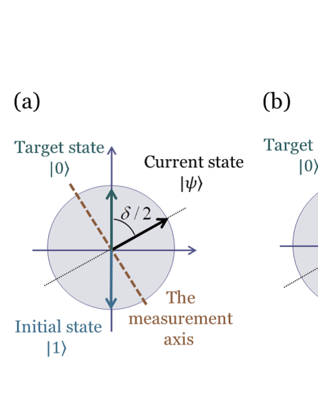
Figure 1: (Color online) The measurement axes of Jacobs’ adaptive measurement scheme (a) and the presented scheme (b).

Here we come up with the question about how much the above adaptive measurement scheme is robust against certain disturbance acting on the system. Actually such robustness against a specific decohering effect was evaluated in JacobsNJP2010 . Another specific but important disturbance is an unknown unitary evolution of the qubit state, in which case the driving term $-i[\hat{H},\hat{\rho}_{t}]dt$ is added to the right hand side of Eq. (I). For example, if we take a two-level atom continuously observed using the Faraday rotation technique Stockton to realize the qubit system subjected to Eq. (I), such a disturbing Hamiltonian may appear and take the form $\hat{H}=\Delta\hat{\sigma}_{y}$ with $\Delta$ unknown detuning between the atomic transition frequency and the laser frequency. Note that in JacobsNJP2010 this kind of unknown disturbance was not discussed.

In this paper, we reconsider the same control problem discussed above, yet with additional care about the influence of an unknown unitary evolution, and then propose a new adaptive measurement scheme that has clear robustness property against that disturbance. A novel difference between our scheme and Jacobs’ one is that we take the measurement axis between the currenet and the target states in the sense shown in Fig. 1 (b), rather than the orthogonal one; then that measurement axis converges to the target, so that the state may be probabilistically moved toward the target as well. The main feature of this scheme is that we can keep the measurement strength constant during all the time-evolution, while in Jacobs’ case it must be weakened when the state approaches to the target. This mechanism brings the following two merits: (i) The first is that the experimental implementation becomes simpler; in fact we need to adaptively change only the measurement axis. (ii) Secondly, because the measurement strength is not weakened, the system preserves capability moving the state via measurement back action even near the target. The latter is more important in the present context, because it is then expected that the adaptive measurement can deal with the unknown force along all the time evolution, while in Jacobs’ case the unknown force has to become dominant and thus cannot be suppressed when the state approaches to the target. This fact will be actually demonstrated in numerical simulations.

II The adaptive measurement scheme

In general, if we continuously measure an observable in a QND manner, the state moves probabilistically toward one of the eigenstates of that observable Handel ; QM . Hence, if this measured observable is changed adaptively so that the eigenstate attracting the current state approaches to a desired target state, it is expected that the state will finally be stabilized at that target state. Based on this idea, we take the following observable as a measured observable in Eq. (I):

$$\hat{\sigma}_{t}^{\rm R}=\hat{\sigma}_{x}\sin(\alpha\delta_{t})+\hat{\sigma}_{z}\cos(\alpha\delta_{t}),$$ (5)

where $\alpha\in[0,1]$ is the tuning parameter whose meaning is explained below. The index “${\rm R}$” indicates that it is the “Robust” adaptive measurement scheme to discern it from Jacobs’ one. The eigenstates of the observable $\hat{\sigma}_{t}^{\rm R}$ are given by

$$|{+_{\rm{Z}}}\rangle=\begin{pmatrix}\cos(\alpha\delta_{t}/2)\\ \sin(\alpha\delta_{t}/2)\end{pmatrix},~{}~{}|{-_{\rm{Z}}}\rangle=\begin{pmatrix}\sin(\alpha\delta_{t}/2)\\ -\cos(\alpha\delta_{t}/2)\end{pmatrix},$$

which satisfy $\hat{\sigma}_{t}^{\rm R}|{+_{\rm Z}}\rangle=|{+_{\rm{Z}}}\rangle,~{}\hat{\sigma}_{t}^{\rm R}|{-_{\rm Z}}\rangle=-|{-_{\rm Z}}\rangle$. In the Bloch sphere representation, $|{+_{\rm{Z}}}\rangle$ divides the angle between the target state $|{0}\rangle$ and the current state $|{\psi_{t}}\rangle=(\cos(\delta_{t}/2),~{}\sin(\delta_{t}/2))^{\top}$ into $\alpha:(1-\alpha)$; see Fig. 1 (b). The transition probabilities of the state jumping to these eigenstates are $p_{+}=|\langle{+_{\rm Z}}|{\psi_{t}}\rangle|^{2}=(1+\cos(\beta\delta_{t})/2$ and $p_{-}=|\langle{-_{\rm Z}}|{\psi_{t}}\rangle|^{2}=(1-\cos(\beta\delta_{t}))/2$, where $\beta:=1-\alpha$, and they satisfy $p_{+}\geq p_{-}$ if $\cos(\beta\delta_{t})\geq 0$. This means that the state tends to move towards the direction of $|{+_{\rm Z}}\rangle$ with probability $p_{+}$. At the same time, since in this case $\delta_{t}$ decreases, the eigenstate $|{+_{\rm{Z}}}\rangle$ moves towards the target $|{0}\rangle$. In particular, when the state reaches the target $|{0}\rangle$, or equivalently $\delta_{t}\rightarrow 0$, the eigenstate $|{+_{\rm Z}}\rangle$ becomes identical to the target and the transition probability $p_{+}$ takes the value $1$; that is, the state is stabilized at the target as expected.

Next, the measurement strength is simply set to a constant value $k_{t}^{\rm R}=k^{\rm R}$, unlike the case of Jacobs’ scheme. The reason will be explained in Remark (i) given in the end of this section, but we here point out that this setting has a clear merit from a practical viewpoint. In fact, changing the measurement strength in addition to changing the measured observable definitely costs more expensive compared to the case where only the latter is required. In this sense, our scheme is suited to experimental implementation.

Regarding the disturbing Hamiltonian, as discussed in Sec. I, we choose $\hat{H}=\Delta\hat{\sigma}_{y}$, where $\Delta$ is an unknown constant. Note that with this Hamiltonian the state rotates around the $y$ axis in the Bloch sphere.

Consequently, the dynamical evolution of the state under the adaptive measurement setup and the disturbing Hamiltonian introduced above is given by

$$d\hat{\rho}_{t}= -i\Delta[\hat{\sigma}_{y},\hat{\rho}_{t}]dt-k^{\rm R}[\hat{\sigma}_{t}^{\rm R},[\hat{\sigma}_{t}^{\rm R},\hat{\rho}_{t}]]dt$$

$$+\sqrt{2k^{\rm R}}\big{(}\hat{\sigma}_{t}^{\rm R}\hat{\rho}_{t}+\hat{\rho}_{t}\hat{\sigma}_{t}^{\rm R}-2{\rm Tr}\hskip 1.9919pt(\hat{\sigma}_{t}^{\rm R}\hat{\rho}_{t})\hat{\rho}_{t}\big{)}dW_{t}.$$ (6)

The initial state is now on the $x$-$z$ plane, hence we have the dynamics of $\delta_{t}$ as follows:

$$d\delta_{t}=2\Delta dt-2k^{\rm{R}}\sin(2\beta\delta_{t})dt+\sqrt{8k^{\rm{R}}}\sin(\beta\delta_{t})dW_{t}.$$ (7)

The linear approximated equation, which is valid when $\delta_{t}\approx 0$, is

$$d\delta_{t}=2\Delta dt-4k^{\rm{R}}\beta\delta_{t}dt+\sqrt{8k^{\rm{R}}}\beta\delta_{t}dW_{t}.$$ (8)

On the other hand, the dynamics of the same $\delta_{t}$ but with Jacobs’ scheme is given by

$$d\delta_{t}=2\Delta dt+\sqrt{8\kappa}\delta_{t}dW_{t}.$$ (9)

A striking difference of the above two dynamics (8) and (9) is that the former contains an additional drift term $-4k^{\rm R}\beta\delta_{t}dt$ while in the latter equation there is no such state-dependent term. Note that this additional drift term apparently works for driving $\delta_{t}$ toward zero. This fine property of our scheme is brought from the mechanism that, around $\delta_{t}=0$, the target state itself is continuously measured and thus the state is attracted to the target with very high probability. In contrast, as mentioned before, in Jacobs’ case the measurement has to be weakened and finally turned off when the state reaches the target, thus there is no such attracting effect changing $\delta_{t}$ to zero. We further expect that the additional drift term in Eq. (8) implies no more than the enhancement of stability of the dynamics of $\delta_{t}$, which consequently makes the system robust against the disturbing noise. Note that this observation makes sense only when the state is around the target. Therefore, in the later sections we will examine some numerical simulations to actually verify the above-mentioned driving effect and resulting robustness property.

Before closing this section, we provide two remarks.

Remark (i): Jacobs’ scheme requires the adaptive tuning of the measurement strength (i.e., $k_{t}^{\rm J}=\kappa\delta_{t}^{2}$ in Eq. (3)) for the dynamics of $\delta_{t}$ to have the state-dependent diffusion term. Such state-dependence is indeed necessary to generate dynamical stability of $\delta_{t}$. Hence, it should be maintained that, with our measurement scheme, the diffusion term of Eq. (7) depends on the state even with the fixed measurement strength (i.e., $k_{t}^{\rm R}=k^{\rm R}$).

Remark (ii): The time evolution of the fidelity between the current state $\hat{\rho}_{t}$ and the target state $|{0}\rangle$ is given by

$$d\langle{0}|\hat{\rho}_{t}|{0}\rangle=\Big{[}-\Delta\sin\delta_{t}+k^{\rm R}\Big{(}\cos(2\alpha\delta_{t}-\delta_{t})-\cos\delta_{t}\Big{)}\Big{]}dt$$

$$-\sqrt{2k^{\rm R}}\Big{[}\frac{3+\cos\delta_{t}}{2}\cos(\alpha\delta_{t}-\delta_{t})+\cos(\alpha\delta_{t})\Big{]}dW_{t}.$$ (10)

Hence, the optimum value of $\alpha$ that maximizes the deterministic change per unit time of the fidelity is given by $\alpha=1/2$. This value is actually taken in the simulations shown later.

III State convergence

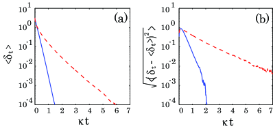
Figure 2: (Color online) Time evolutions of (a) the mean and (b) the standard deviation of $\delta_{t}$ when $\Delta=0$. The solid blue line corresponds to our adaptive measurement scheme while the dashed red line does Jacobs’ scheme.

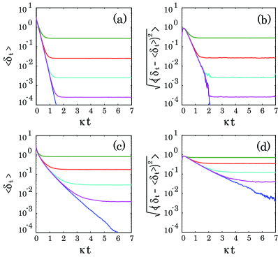
Figure 3: (Color online) Time evolutions of (a) the mean and (b) the standard deviation of $\delta_{t}$ subjected to our scheme, for several values of $\Delta$. The green, red, water blue, purple, and blue lines correspond to $\Delta=1,1/10,1/10^{2},1/10^{3}$, and $\Delta=0$, respectively.

In this section, to verify that our adaptive measurement scheme actually works for driving the state towards the target, we examine some numerical simulations, under the assumption that $\Delta$ is known; this is a crucial assumption because we are then able to update $\delta_{t}$ and as a result the adaptive measurement law (5) (or Eq. (3)) exactly by recursively solving Eq. (7) (or Eq. (9) for Jacobs’ case). For reference, we show the trajectories in Jacobs’ case as well; in particular, we set the same diffusion coefficients in Eqs. (8) and (9); i.e., $\sqrt{8k^{\rm R}}\beta=\sqrt{8\kappa}$, which leads to $k^{\rm R}\beta^{2}=\kappa$. Hence let us here take the parameters as $\kappa=1$, $k^{\rm R}=4$, and $\alpha=1-\beta=1/2$ (see Remark (ii) in Sec. II). The disturbance strength $\Delta$ takes several values. The initial condition is $\delta_{0}=\pi$, as defined below Eq. (2).

Figure 2 shows the time evolutions of the mean and the standard deviation of $\delta_{t}$, when $\Delta=0$. The plots are obtained by averaging $10^{6}$ sample paths. The solid blue and the dashed red lines correspond to the cases of our adaptive measurement scheme and Jacobs’ one, respectively. We find from the figures that, in both cases, the state certainly converges to the target with almost probability one. Note that the plots do not imply that our scheme offers faster and stable convergence of the state compared to Jacobs’ case; this is because the measurement strength of Jacobs’ scheme has to be weakened, implying slower change of the state around the target.

Next, Fig. 3 shows the means and the standard deviations of $\delta_{t}$, with several values of $\Delta$. As expected, the disturbance prevents the state from converging to the target. Notably, in the long time limit, the error is approximately proportional to $\Delta$. Similar plots are obtained in Jacobs’ case as well.

Remark: Although we mentioned above that the figures do not imply the superiority of our scheme over Jacobs’ one, a trivial fair comparison can be performed as follows. In fact, if we take a constant measurement strength $k_{t}^{\rm J}=k^{\rm J}$ in Jacobs’ scheme, the dynamics is given by $d\delta_{t}=\sqrt{8k^{\rm J}}dW_{t}$; clearly, then, $\delta_{t}$ does not converge to zero even under the boundary condition. That is, if we run the two schemes with the same constant measurement strength, clearly our scheme offers better performance over Jacobs’ one.

IV Robustness of the adaptive Zeno measurement

Here we study the case where the disturbance magnitude $\Delta$ is unknown. To make the situation clear, let us again consider the general SME (I) that is additionally driven by an unknown Hamiltonian $\hat{H}$:

$$d\hat{\rho}_{t}= -i[\hat{H},\hat{\rho}_{t}]dt-k_{t}\big{[}\hat{\sigma}_{t},[\hat{\sigma}_{t},\hat{\rho}_{t}]\big{]}dt$$

$$+\sqrt{2k_{t}}\big{[}\hat{\sigma}_{t}\hat{\rho}_{t}+\hat{\rho}_{t}\hat{\sigma}_{t}-2{\rm Tr}\hskip 1.9919pt(\hat{\sigma}_{t}\hat{\rho}_{t})\hat{\rho}_{t}\big{]}dW_{t}.$$ (11)

This true state $\hat{\rho}_{t}$ cannot be precisely updated, due to the uncertainty of $\hat{H}$. Therefore, we need to devise an updating law of a nominal state, say $\hat{\rho}_{t}^{\prime}$, only using the measurement result $y_{t}$ that is subjected to the output equation

$$dy_{t}={\rm Tr}\hskip 1.9919pt(\hat{\sigma}_{t}\hat{\rho}_{t})dt+dW_{t}.$$ (12)

Note this is driven by the same $dW_{t}$ as that in Eq. (IV); $dW_{t}$ is called the innovation in the framework of quantum filtering theory Belavkin ; Bouten . To update $\hat{\rho}_{t}^{\prime}$, we particularly use Eqs. (IV) and (12) with $\hat{H}$ replaced by a known nominal Hamiltonian $\hat{H}^{\prime}$ as follows:

$$d\hat{\rho}^{\prime}_{t}= -i[\hat{H}^{\prime},\hat{\rho}_{t}^{\prime}]dt-k_{t}\big{[}\hat{\sigma}_{t},[\hat{\sigma}_{t},\hat{\rho}^{\prime}_{t}]\big{]}dt$$

$$+\sqrt{2k_{t}}\big{[}\hat{\sigma}_{t}\hat{\rho}^{\prime}_{t}+\hat{\rho}^{\prime}_{t}\hat{\sigma}_{t}-2{\rm Tr}\hskip 1.9919pt(\hat{\sigma}_{t}\hat{\rho}^{\prime}_{t})\hat{\rho}^{\prime}_{t}\big{]}$$

$$\hskip 30.00005pt\times[dy_{t}-{\rm Tr}\hskip 1.9919pt(\hat{\sigma}_{t}\hat{\rho}^{\prime}_{t})dt].$$ (13)

Note again that $y_{t}$ is the measurement result and is thus known. Hence we can recursively calculate the nominal state $\hat{\rho}_{t}^{\prime}$, although it should differ from the true state $\hat{\rho}_{t}$. In the adaptive measurement setup, therefore, the observable $\hat{\sigma}_{t}$ and the strength $k_{t}$ are changed in time as functions of $\hat{\rho}_{t}^{\prime}$.

For the specific problem under consideration, let $\hat{H}=\Delta\hat{\sigma}_{\rm y}$ and $\hat{H}^{\prime}=\Delta^{\prime}\hat{\sigma}_{\rm y}$ be the true and nominal Hamiltonians, respectively; $\Delta$ is an unknown constant while $\Delta^{\prime}$ is a known nominal constant. Also we define $\delta_{t}$ and $\delta^{\prime}_{t}$, corresponding to the true and the nominal states. In our measurement scheme, these variables are driven by the following equations:

$$d\delta_{t}=\big{[}2\Delta-2k^{\rm Z}\sin(2\delta_{t}-2\alpha\delta_{t}^{\prime})\big{]}dt$$

$$\hskip 10.00002pt\mbox{}+\sqrt{8k^{\rm Z}}\sin(\delta_{t}-\alpha\delta_{t}^{\prime})dW_{t},$$ (14)

$$d\delta_{t}^{\prime}=\big{[}2\Delta^{\prime}-2k^{\rm Z}\sin(2\beta\delta_{t}^{\prime})\big{]}dt$$

$$\hskip 10.00002pt\mbox{}+\sqrt{8k^{\rm Z}}\sin(\beta\delta_{t}^{\prime})dW_{t}^{\rm Z},$$ (15)

where

$$dW_{t}^{\rm Z}=\big{[}\cos(\beta\delta_{t}^{\prime})-\cos(\delta_{t}^{\prime}-\alpha\delta_{t})\big{]}dt+dW_{t}.$$

Note that $\beta=1-\alpha$. The above two equations (IV) and (IV) take the same form when $\Delta=\Delta^{\prime}$ and $\delta_{t}=\delta_{t}^{\prime}$. Jacobs’ scheme, on the other hand, leads to the following equations to update $\delta_{t}$ and $\delta_{t}^{\prime}$:

$$d\delta_{t}=\big{[}2\Delta+2\kappa\delta_{t}^{\prime}\mbox{}^{2}\sin(2\delta_{t}-2\delta_{t}^{\prime})\big{]}dt$$

$$\hskip 10.00002pt\mbox{}+\sqrt{8\kappa}\delta_{t}^{\prime}\cos(\delta_{t}-\delta_{t}^{\prime})dW_{t},$$ (16)

$$d\delta_{t}^{\prime}=2\Delta^{\prime}dt+\sqrt{8\kappa}\delta_{t}^{\prime}dW_{t}^{\rm J},$$ (17)

where

$$dW_{t}^{\rm J}=\sin(\delta_{t}^{\prime}-\delta_{t})dt+dW_{t}.$$

Again, the above two equations (IV) and (17) take the same form when $\Delta=\Delta^{\prime}$ and $\delta_{t}=\delta_{t}^{\prime}$.

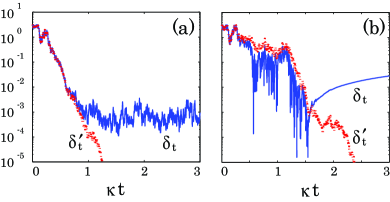
Figure 4: (Color online) Sample paths of the true variable $\delta_{t}$ (solid blue lines) and the nominal one $\delta_{t}^{\prime}$ (dashed red lines) for (a) our adaptive measurement scheme and (b) Jacobs’ scheme, where $\Delta=1/10^{2}$ and $\Delta^{\prime}=0$.

In Fig. 4 we show sample paths of $\delta_{t}$ (solid blue line) and $\delta_{t}^{\prime}$ (dashed red line) for both of the adaptive measurement schemes, with the same parameters taken in Sec. III, fixed uncertainty $\Delta=1/10^{2}$, and a typical nominal value $\Delta^{\prime}=0$. We find from the figures that, with our adaptive measurement scheme, the true variable $\delta_{t}$ is stabilized around the target $\delta_{t}=0$ though it still has a certain error corresponding to the constant external force, while in Jacobs’ scheme $\delta_{t}$ finally follows a deterministic time-evolution and goes away from zero; in every numerical simulation a similar behavior is observed.

We here address the mechanism that brings about the above drastic difference. First, since the nominal state is now governed by the dynamics without uncertainty, $\delta_{t}^{\prime}$ converges to zero, as seen in Sec. III. When $\delta_{t}^{\prime}\rightarrow 0$, the measured observable becomes $\hat{\sigma}_{t}=\hat{\sigma}_{z}$ for both the adaptive measurement schemes, but the measurement strength becomes $k_{t}^{\rm J}=0$ for Jacobs’ case while $k_{t}^{R}=k^{\rm R}$ in our case; that is, Jacobs’ scheme stops to measure the system once $\delta_{t}^{\prime}=0$ is reached, and consequently the true variable $\delta_{t}$ turns out to follow the deterministic dynamics $d\delta_{t}/dt=2\Delta$. In contrast, our scheme keeps measuring $\sigma_{z}$, even after $\delta_{t}^{\prime}$ takes zero, implying that the true state can be stabilized around the target.

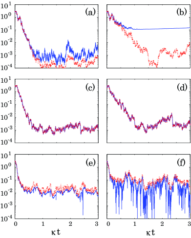
Figure 5: (Color online) Sample paths of the true variable $\delta_{t}$ (solid blue lines) and the nominal one $\delta_{t}^{\prime}$ (dashed red lines) for (a, c, e) the presented adaptive measurement scheme and (b, d, f) Jacobs’ scheme. For all cases, the true external force is set to $\Delta=1/10^{2}$, while several nominal values of $\Delta^{\prime}$ are examined: (a, b) represent the case when $\Delta^{\prime}=1/10^{3}$, (c, d) for the case $\Delta^{\prime}=1/10^{2}$, and (e, f) for the case $\Delta^{\prime}=1/10$.

The above statement holds only for the case of $\Delta^{\prime}=0$; hence we take some non-zero values of $\Delta^{\prime}$ and show in Fig. 5 the trajectories of $\delta_{t}$ and $\delta_{t}^{\prime}$. If $\Delta^{\prime}$ is not zero but smaller than the true value $\Delta$ (Figs. 5 (a, b)), we observe similar trajectories to the case of $\Delta^{\prime}=0$; that is, in Jacobs’ case the true variable again goes away from zero deterministically, due to the same reason stated above. In Figs. 5 (c, d) where $\Delta=\Delta^{\prime}$, the nominal variable $\delta_{t}^{\prime}$ exactly tracks $\delta_{t}$, which is the property the nominal updating laws (IV) and (17) should have. Lastly, if $\Delta^{\prime}$ is bigger than $\Delta$ (Figs. 5 (e, f)), or in other words if we take a conservative approach for estimating $\delta_{t}$, Jacobs’ scheme can stabilize the state around the target although it has big fluctuation, while our measurement scheme moves the state more close towards zero with much smaller estimation error.

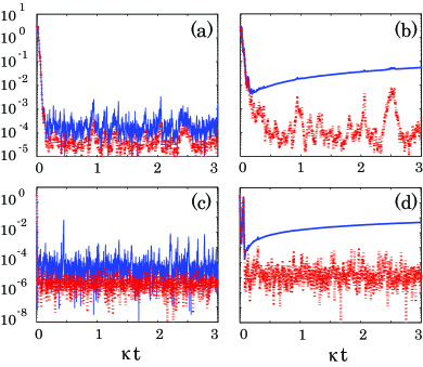
Figure 6: (Color online) Sample paths of the true variable $\delta_{t}$ (solid blue lines) and the nominal one $\delta_{t}^{\prime}$ (dashed red lines) for (a, c) the presented adaptive measurement scheme and (b, d) Jacobs’ scheme. For all cases, we set $\Delta=1/10^{2}$ and $\Delta^{\prime}=1/10^{3}$. The measurement strength is taken as $\kappa=5$ for the cases (a, b) while $\kappa=50$ for (c, d).

We further expect that the issue found in Jacobs’ case may be avoided by taking a large value of $\kappa$; actually, the major drawback of Jacobs’ scheme is that the measurement strength has to be weakened around the target, which brings less stability of the state. Hence let us try some larger values of $\kappa$ to see if a similar issue can still happen. Figures 6 (b, d) demonstrate the nominal and true valus of $\delta_{t}$ in Jacobs’ case, with the parameters $\Delta=1/10^{2}$ and $\Delta^{\prime}=1/10^{3}$; in particular, here a relatively large values of $\kappa$ are taken, i.e., $\kappa=5$ for the case (b) and $\kappa=50$ for the case (d). Clearly, the stability are enhanced compared to the previous cases shown in Fig. 5 in the sense that the convergence speed becomes faster. However, the issue is not resolved; that is, in both cases the nominal state fails to track the true one once it approaches to the target, and then the true one obeys the deterministic unitary time evolution and flows away from the target. On the other hand, as shown in Figs. 6 (a, c), our measurement scheme does not bring such flow of the state, because of the intrinsic stability given to both $\delta_{t}$ and $\delta_{t}^{\prime}$. Note that, when $\Delta^{\prime}>\Delta$, the issue observed in Fig. 5 (f) still happens, while in our case the fluctuation is well suppressed.

Summarizing, our adaptive measurement scheme offers better estimation of $\delta_{t}$, compared to Jacobs’ case, in the sense that it is fairly robust against the uncertainty of the additional unitary time evolution. It should be maintained again that this nice stability property is brought from the mechanism of continuous monitoring of the system with constant measurement strength.

V Concluding remarks

The main features of the presented adaptive measurement scheme are twofold; the first is that the measured observable contains an eigenstate that eventually converges to the target state, and the other is that the measurement strength can be taken constant even when the state is close to the target, which is the crucial property bringing the robustness property. As long as the above two conditions are satisfied, it is expected that our measurement scheme can be generalized to the multi-dimensional case. However, in many situations any physically available observable does not contain an eigenvector that is identical to a desired target state, and then our measurement scheme cannot be used for preparing that target state. Rather, as discussed in AshhabPRA2010 ; WisemanNature2011 , in such a case, a certain weak measurement may work for generating a target state. But a critical requirement for this measurement is that the measurement strength should be weakened when the state approaches to the target; then, the system can become fragile against unknown disturbance, as seen in Sec. IV. Exploring an adaptive measurement method that overcomes this issue is an interesting future work.

We thank Yuzuru Kato for his contribution to Remark (ii) in Sec. II.

References

- (1) H. M. Wiseman, Phys. Rev. Lett. 75, 4587 (1995); H. M. Wiseman and R. B. Killip, Phys. Rev. A 56, 944 (1997); H. M. Wiseman and R. B. Killip, Phys. Rev. A 57, 2169 (1998); D.W. Berry and H. M. Wiseman, Phys. Rev. Lett. 85, 5098 (2000); D.W. Berry and H. M. Wiseman, Phys. Rev. A 65, 043803 (2002).
- (2) M. A. Armen et al., Phys. Rev. Lett. 89, 133602 (2002).
- (3) M. Tsang, J. H. Shapiro, and S. Lloyd, Phys. Rev. A 79, 053843 (2009).
- (4) T. A. Wheatley, et. al., Phys. Rev. Lett. 104, 093601 (2010).
- (5) H. Yonezawa, et. al., Science 337, 1514 (2012).
- (6) K. Jacobs, New J. Phys. 12, 043005, (2010).
- (7) S. Ashhab and F. Nori, Phys. Rev. A , 82, 06103 (2010).
- (8) H. M. Wiseman, Nature 470, 178 (2011).
- (9) F. Ciccarello, M. Paternostro, M. S. Kim, and G. M. Palma, Phys. Rev. Lett. 100, 150501 (2008).
- (10) K. Yuasa, D. Burgarth, V. Giovannetti, and H. Nakazato, New J. Phys. 11, 123027 (2009).
- (11) R. Van Handel, J. K. Stockton, and H. Mabuchi, IEEE Trans. Automat. Contr. 50, 768/780 (2005).
- (12) H. M. Wiseman and G. J. Milburn, Quantum measurement and Control (New York, Cambridge University Press, 2010).
- (13) J. K. Stockton, Continuous Quantum Measurement of Cold Alkali-Atom Spins, Ph.D Thesis, California Institute of Technology, 2006.
- (14) V. P. Belavkin, J. Multivariate Anal. 42, 171/201 (1992).
- (15) L. Bouten, R. van Handel, and M. R. James, SIAM J. Control Optim. 46, 2199/2241 (2007).