Stabilizing single- and two-color vortex beams in quadratic media by a trapping potential

Abstract

We consider two-dimensional (2D) localized modes in the second-harmonic-generating ($\chi^{(2)}$) system with the harmonic-oscillator (HO) trapping potential. In addition to its realization in optics, the system describes the mean-field dynamics of mixed atomic-molecular Bose-Einstein condensates (BECs). The existence and stability of various modes is determined by their total power, $N$, topological charge, $m/2$ [$m$ is the intrinsic vorticity of the second-harmonic (SH) field], and $\chi^{(2)}$ mismatch, $q$. The analysis is carried out in a numerical form and, in parallel, by means of the variational approximation (VA), which produces results that agree well with numerical findings. Below a certain power threshold, $N\leq N_{c}^{(m)}(q)$, all trapped modes are of the single-color type, represented by the SH component only, while the fundamental-frequency (FF) one is absent. In contrast with the usual situation, where such modes are always unstable, we demonstrate that they are stable, for $m=0,1,2$ (the mode with $m=1$ may be formally considered as a semi-vortex with topological charge $m/2=1/2$), at $N\leq N_{c}^{(m)}(q)$, and unstable above this threshold. On the other hand, $N_{c}^{(m)}(q)\equiv 0$ at $q\geq q_{\max}$ (in our notation, $q_{\max}=1$), hence the single-color modes are unstable in the latter case. At $N=N_{c}^{(m)}$, the modes with $m=0$ and $m=2$ undergo a pitchfork bifurcation, which gives rise to two-color states, which remain completely stable for $m=0$. The two-color vortices with $m=2$ (topological charge $1$) have an upper stability border, $N=N_{c2}(q)$. Above the border, they exhibit periodic splittings and recombinations, while keeping their vorticity. The semi-vortex does not bifurcate; at $N=N_{c}^{(m=1)}$, it exhibits quasi-chaotic oscillations and a rotating “groove” resembling a screw-edge dislocation induced by the semi-integer vorticity.

OSIS numbers: 190.6135; 190.3100; 190.4410; 020.475

I Introduction

It is commonly known that the quadratic, alias $\chi^{(2)}$, nonlinearity, plays a fundamental role in nonlinear optics, helping, in particular, to create various species of solitons review0 -review , KA . The use of the $\chi^{(2)}$ nonlinearity is crucially important for the making of 2D and 3D solitons, because, on the contrary to Kerr ($\chi^{(3)}$) nonlinearity, the quadratic interaction between the FF and SH fields does not give rise to the collapse Rubenchik , which is a severe problem for the stability of 2D and 3D solitons in Kerr media review . Thanks to this circumstance, the first $\chi^{(2)}$ solitons were created as stable (2+1)-dimensional beams propagating in an SH-generating crystal first-exper . Further, the absence of the collapse instability in the 3D setting suggests a possibility of creating fully localized “light bullets” Drummond . In the experiment, 3D solitons have not been observed yet, the best result being a spatiotemporal soliton self-trapped in the longitudinal and one transverse directions, due to the interplay of the diffraction, group-velocity dispersion, and $\chi^{(2)}$ nonlinearity, while the confinement in the other transverse direction was provided by the waveguiding structure Wise1 ; Wise2 .

Another natural possibility in the (2+1)D setting is the creation of vortical solitary beams, with the “hollow” in the middle. In these modes, self-trapped SH and FF fields carry intrinsic vorticities $m$ and $m/2$, respectively. The modes are classified as vortex solitons with topological charge $m/2$; solitons with odd values of $m$ are not possible, as the intrinsic vorticity of the FF component, $m/2$, cannot take half-integer values, although vortices with a half-integer optical angular momentum can be created, in the form of mixed screw-edge dislocations, by passing the holding beam through a spiral-phase plate displaced off the beam’s axis half . Unlike their fundamental counterparts with $m=0$, the vortex solitons in the free space are always unstable against azimuthal perturbations, which split them into sets of separating segments. This instability was predicted theoretically splitting1 -splitting5 and demonstrated in the experiment splitting-exp . The same instability was also predicted in the framework of the so-called Type-II (three-wave) $\chi^{(2)}$ system, which includes two distinct components of the FF field splitting-3W ; splitting-3W2 .

Solitons with embedded vorticity are also known as solutions to the 2D nonlinear Schrödinger (NLS) equation with the self-focusing cubic term Kruglov , and they too are subject to the azimuthal instability, which is actually stronger than the collapse-induced instability review . The 2D self-focusing NLS equation models not only the light transmission in bulk media with the Kerr nonlinearity, but also [in the form of the Gross-Pitaevskii (GP) equation] the mean-field dynamics of BECs in ultracold gases with attractive inter-atomic interactions, shaped as “pancakes” by the confining potential BEC . A solution to the instability problem was elaborated in the latter context: both fundamental solitons and solitary vortices with topological charge $1$ can be stabilized by isotropic HO (harmonic-oscillator) trapping potentials. As shown in detail in a number of theoretical works cubic-in-trap1 -cubic-in-trap7 , the HO potential stabilizes the fundamental solitons in the entire region of their existence, while vortex solitons are stabilized, in terms of their norm (the counterpart of the total power of spatial optical solitons), in $\simeq 33\%$ of their existence region, and in an adjacent region of width $\simeq 10\%$ vortices exist in the form of periodically splitting and recombing modes, which keep their vorticity cubic-in-trap5 .

The effective 2D trapping potential can be also realized in optical waveguides, in the form of the respective profile of the transverse modulation of the local refractive index KA . This circumstance suggests a natural possibility for the stabilization of (2+1)D vortex solitons in the $\chi^{(2)}$ medium by means of the radial HO potential, which is the main subject of the present work. A feasible approach to the making of the optical medium combining a nearly-parabolic profile of the refractive index and $\chi^{(2)}$ nonlinearity is the use of a 2D photonic crystal, which can be readily designed to emulate the required index profile, while the nonlinearity is provided by the poled material (liquid Du or solid Luan ) filling the voids. As shown below, the effective radial potential provides for sufficiently strong localization of the trapped modes, therefore the exact parabolic shape of the radial profile is not crucially important. The analysis can be readily adjusted to other profiles, if necessary.

The model, based on the system of coupled equations for the FF and SH fields, is introduced in Section II. It is relevant to mention that essentially the same system of GP equations for the atomic and molecular mean-field wave functions describes the BEC in the atomic-molecular mixture BEC0 -BEC4 . Accordingly, the predicted mechanism of the stabilization of two-component vortex solitons trapped in the HO potential can also be realized in the BEC mixture.

Solutions for the trapped 2D modes and their stability against perturbations are considered in Sections III and IV. First, we address states which, in the unperturbed form, contain only the SH field, while the FF component vanishes. Such single-color solutions of the $\chi^{(2)}$ system are known in other contexts, but they are usually subject to the parametric instability against small perturbations in the FF component. Our first result is that the trapped single-color modes, both fundamental and vortical ones, have a finite stability domain. In particular, the single-color modes with $m=1$, which (formally) look as semi-vortices with topological charge $1/2$, are also found, and they are stable too in a finite parameter area. The single-color states become unstable at a particular critical value of the total power (alias norm); however, the critical norm vanishes if the mismatch parameter, $q$, is too large, viz., at $q>1$ in the notation adopted below). As concerns the fundamental modes ($m=0$) and those with topological charge $1$ ($m=2$), at exactly the same critical point they undergo a pitchfork bifurcation, which gives rise to two-color states. The stability of the fundamental two-color mode is obvious, while a nontrivial result is finding stability borders for the trapped two-color vortex soliton. Above the instability border, it develop periodic oscillations, keeping its vorticity and featuring periodic splittings and recoveries. As concerns the single-color semi-vortex, it exhibits a different behavior, developing persistent quasi-random oscillations above the stability border, mixing the first and zeroth angular harmonics in both the SH and FF components.

The results concerning the shape and stability of the modes of all the above-mentioned types (single-color ones with $m=0,1,2$, and two-color complexes with $m=0$ and $2$) are obtained, in parallel, by means of numerical methods and in an analytical form, based on the variational approximation (VA). In almost all the cases, the VA demonstrates very good accuracy in comparison with numerical results.

II The model

The model for the SH generation in 2D is based on the usual scaled equations review0 -review2 for the FF and SH field amplitudes, $u$ and $v$,

$$i\frac{\partial u}{\partial z}+\frac{1}{2}\left(\frac{\partial^{2}}{\partial x^{2}}+\frac{\partial^{2}}{\partial y^{2}}\right)u+u^{\ast}v-U(x,y)u = 0,$$

$$2i\frac{\partial v}{\partial z}+\frac{1}{2}\left(\frac{\partial^{2}}{\partial x^{2}}+\frac{\partial^{2}}{\partial y^{2}}\right)v-qv+\frac{1}{2}u^{2}-4U(x,y)v = 0,$$ (1)

where $z$ is the propagation distance, $x$ and $y$ are the transverse coordinates, the asterisk stands for the complex conjugate, $q$ is the real mismatch coefficient, and, as said above, the axisymmetric modulation of the refractive index is modeled by the isotropic HO potential, $U(x,y)=\left(\Omega^{2}/2\right)\left(x^{2}+y^{2}\right)$. By means of an obvious rescaling, we fix $\Omega=1/2$, while $q$ remains a free parameter.

The relation between the potential terms in the equation for the FF and SH fields implies that the same refractive index acts on both fields, which is a realistic assumption for materials of which the above-mentioned pair of the photonic crystal and voids-filling stuff can be fabricated. If the weak index dispersion is taken into regards, it will produce only a small perturbation in the system.

The 2D system of scaled GP equations for the atomic-molecular mixture corresponds to Eqs. (1) with $z$ replaced by time $t$, and $q$ accounting for a difference of the chemical potential between the atomic and molecular components, $u$ and $v$. It is relevant to mention that a similar model with a spatially periodic (lattice) potential $U\left(x,y\right)$ was considered in Ref. chi2-in-lattice , where it was demonstrated that the lattice can readily stabilize two-color solitary vortices, although with an anisotropic shape.

Equations (1) are derived from the corresponding action, $S=\int Ldz$, with Lagrangian

$$L = \int\int\left\{\left[iu_{z}u^{\ast}+2iv_{z}v^{\ast}-\frac{1}{2}\left(|u_{x}|^{2}+|u_{y}|^{2}+|v_{x}|^{2}+|v_{y}|^{2}\right)\right]\right.$$ (2)

$$\left.-U(r)\left(|u|^{2}+4|v|^{2}\right)-q|v|^{2}+\frac{1}{2}\left(u^{2}v^{\ast}+u^{2\ast}v\right)\right\}dxdy.$$

Stationary modes can be characterized by their total power (norm), $N=\int\int\left(|u|^{2}+4|v|^{2}\right)dxdy$.

III Stability of single-color beams

III.1 The beams with topological charge $0$ and $1$ ($m=0$ and $m=2$)

For the single-color modes with $u=0$, the SH field satisfies the 2D linear Schrödinger equation with the isotropic HO potential,

$$2i\frac{\partial v}{\partial z}+\frac{1}{2}\left(\frac{\partial^{2}}{\partial x^{2}}+\frac{\partial^{2}}{\partial y^{2}}\right)v-qv-4U(x,y)v=0.$$ (3)

Stationary solutions to Eq. (3) are commonly known from quantum mechanics. In polar coordinates $\left(r,\theta\right)$, they are

$$v=v_{m0}\exp\left(i\left(-\mu z+m\theta\right)\right)r^{m}\exp\left(-r^{2}/2\right),$$ (4)

with arbitrary amplitude $v_{m0}$ (it is defined to be real), integer orbital quantum number $m$ (as said above, it corresponds to the beam’s topological charge $m/2$), and eigenvalue $\mu=\left(m+1+q\right)/2$ (recall $\Omega=1/2$ is fixed). The total power of this solution is

$$N_{m}=4\pi m!v_{m0}^{2}.$$ (5)

Solutions (4) are obviously stable within the framework of linear equation (3), the issue being to find a threshold, $N=N_{c}^{(m)}(q)$, at which the parametric instability against infinitesimal perturbations in the FF field sets in, due to the nonlinearity in Eq. (1) for the FF field. As shown in Fig. 1(a), the threshold was identified from systematic simulations of the perturbed evolution of the single-color beams within the framework of the full system of Eqs. (1), for $m=0$ and $2$.

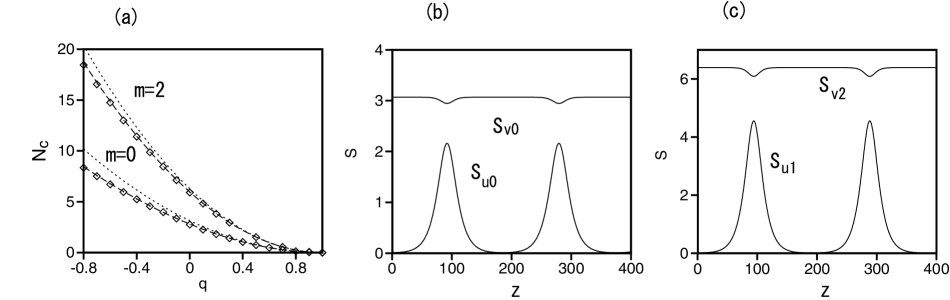
Figure 1: (a) The critical power for the onset of the parametric instability of the single-color beams with topological charges $0$ ($m=0$) and $1$ ($m=2$), the beams being unstable at $N>N_{c}$. Chains of rhombuses and dashed and dotted curves show, respectively, numerical results and the prediction of the variational approximation produced by Eqs. (10), (13), and (14). Examples of periodic oscillations of perturbed solutions at $N>N_{c}$ are shown for $m=0,q=0$, and $N=3$ in (b), and for $m=2$, $q=0$, and $N=6.5$ in (c). Amplitudes $S_{u0,v0}(z)$ and $S_{u1,v2}$ are defined by Eqs. (15) and (16), respectively.

The stability was also investigated in an analytical form by means of the VA. For $m=0$, the ansatz for the perturbed solution is taken as

$$u=u_{0}(z)\exp\left(-\alpha r^{2}\right),~{}v=v_{0}(z)\exp\left(-r^{2}/2\right),$$ (6)

where amplitudes $u_{0}(z)$ and $v_{0}(z)$ are treated as variational parameters, while $\alpha$ is a free constant, which is used below as a variational parameter too, but in a different sense. The substitution of ansatz (6) into Lagrangian (2) leads, after straightforward calculations, to the following Euler-Lagrange equations for variables $u_{0}(z)$ and $v_{0}(z)$:

$$i\frac{du_{0}}{dz} = \left(\alpha+\frac{1}{16\alpha}\right)u_{0}-\frac{4\alpha}{4\alpha+1}u_{0}^{\ast}v_{0},$$ (7)

$$i\frac{dv_{0}}{dz} = \left(\frac{1}{2}+\frac{q}{2}\right)v_{0}-\frac{2}{4\alpha+1}u_{0}^{2}\text{.}$$ (8)

The unperturbed single-color solution to Eqs. (7), (8), $u_{0}=0$, $v_{0}(z)=v_{00}\exp\left(-\left(i/2\right)\left(1+q\right)z\right)$, coincides with exact solution (4) (with $m=0$). Further, to investigate the onset of the parametric instability against the excitation of the infinitesimal FF perturbation, we linearize Eq. (7) and substitute $u_{0}(z)\equiv u_{0}^{\prime}(z)\exp\left(-\left(i/4\right)\left(1+q\right)z\right)$, which leads to the following equation for the perturbation’s amplitude:

$$i\frac{du_{0}^{\prime}}{dz}=\left(\alpha+\frac{1}{16\alpha}-\frac{1}{4}-\frac{q}{4}\right)u_{0}^{\prime}-\frac{4\alpha}{4\alpha+1}v_{00}\left(u_{0}^{\prime}\right)^{\ast}.$$ (9)

An elementary consideration of Eq. (9) demonstrates that it gives rise to the parametric instability at $\left[\alpha+1/(16\alpha)-1/4-q/4\right]^{2}<16\alpha^{2}/(4\alpha+1)^{2}v_{00}^{2}$, hence the critical value of total power (5) is

$$N_{c}^{(m=0)}=4\pi\left(\alpha+\frac{1}{16\alpha}-\frac{1}{4}-\frac{q}{4}\right)^{2}\left(\frac{4\alpha+1}{4\alpha}\right)^{2}.$$ (10)

A similar stability analysis can be performed for the vortical single-color beam (4) with $m=2$. In this case, the natural ansatz for the FF perturbation is taken in the form of the first angular harmonic, i.e.,

$$u=u_{1}^{\prime}(z)r\exp\left[-\alpha r^{2}+i\theta-\left(i/4\right)\left(3+q\right)z\right],$$ (11)

which, after straightforward calculations, leads to the following evolution equation [cf. Eq. (9)]:

$$i\frac{du_{1}^{\prime}}{dz}=\left(2\alpha+\frac{1}{8\alpha}-\frac{3}{4}-\frac{q}{4}\right)u_{1}^{\prime}-\frac{64\alpha^{2}}{(4\alpha+1)^{3}}v_{20}\left(u_{1}^{\prime}\right)^{\ast}.$$ (12)

Taking into regard expression (5), Eq. (12) yields the critical power,

$$N_{c}^{(m=2)}=\frac{\pi(4\alpha+1)^{6}}{512\alpha^{4}}\left(2\alpha+\frac{1}{8\alpha}-\frac{3}{4}-\frac{q}{4}\right)^{2}.$$ (13)

The final analytical prediction for the destabilization thresholds is obtained by the minimization of each expression, (10) and (13) with respect to the variation of free parameter $\alpha$, for given $q$. In particular, an explicit result of the minimization is that, in both cases of $m=0$ and $m=2$,

$$\begin{array}[]{c}N_{c}^{(m=0,2)}\equiv 0~{}~{}\mathrm{at}~{}~{}q\geq 1,\\ N_{c}^{(m=0,2)}\approx\pi\left[1+(m/2)\right]\left(1-q\right)^{2}~{}~{}\mathrm{at}~{}~{}0<1-q\ll 1.\end{array}$$ (14)

The so obtained critical values of $N_{c}$ are shown in Fig. 1(a) by dashed lines, which approximate the numerical results very accurately. Note that Eq. (14) explains the vanishing of $N_{c}$ at $q>1$, which is obvious in Fig. 1(a).

As concerns the realization of the instability in the optical waveguide, it is relevant to note that its length is finite (and usually not very large) in a real experiment. For this reason, the observable instability threshold may be shifted to somewhat larger values of $N$, as a very small instability growth rate would not be able to manifest itself on a relatively short propagation distance.

Above the instability threshold, i.e., at $N>N_{c}^{(m)}$, simulations of both Eqs. (1) and VA equations, (7) and (8), demonstrate oscillatory behavior of perturbed solutions. An example is displayed in Fig. 1(b), at $m=0$, $q=0$, and $N=3$, for variables which, essentially, measure the amplitudes of the zeroth angular harmonic in the FF and SH fields:

$$S_{u0,v0}(z)\equiv\left|\int\int\left\{u\left(x,y\right),v\left(x,y\right)\right\}dxdy\right|.$$ (15)

It is observed in the figure that the unperturbed state with the zero FF amplitude is periodically recovered. A similar example for $m=2$, $q=0$, and $N=6.5$ is displayed in Fig. 1(c), for the integral amplitudes of the first and second angular harmonics in the FF and SH fields, respectively:

$$S_{u1,v2}(z)\equiv\left|\int\int\left\{u\left(x,y\right)e^{-i\theta},v\left(x,y\right)e^{-2i\theta}\right\}dxdy\right|.$$ (16)

III.2 Half-vortices: the beams with topological charge $1/2$ ($m=1$)

A noteworthy peculiarity of the single-color beams (4) is that they may have $m=1$, which formally correspond to the topological charge $m/2\equiv 1/2$. Of course, this is only possible due to the fact that the FF field is absent in the stationary solution; nevertheless, it is shown in what follows below that the half-integer charge of the unperturbed solution essentially affects the perturbed evolution of the single-color vortex above the instability threshold.

To test the stability of these half-vortices within the framework of the VA, a natural ansatz for the FF perturbation is defined as a combination of the zeroth and first angular harmonics: $u=u_{0}^{\prime}\exp\left(-\alpha r^{2}-i\gamma z\right)+u_{1}^{\prime}r\exp\left(-\alpha^{\prime}r^{2}+i\theta-i\gamma^{\prime}z\right)$, with $\gamma$ and $\gamma^{\prime}$ related by the necessary matching condition,

$$\gamma+\gamma^{\prime}=1+q/2.$$ (17)

The VA gives rise to linear coupled equations for perturbation amplitudes $u_{0}^{\prime}$ and $u_{1}^{\prime}$ [cf. Eqs. (9) and (12)]:

$$\gamma u_{0}^{\prime} = \left(\alpha+\frac{1}{16\alpha}\right)u_{0}^{\prime}-\frac{4\alpha}{2\left(\alpha+\alpha^{\prime}\right)+1}v_{10}\left(u_{1}^{\prime}\right)^{\ast},$$

$$\gamma^{\prime}u_{1}^{\prime} = \left(2\alpha^{\prime}+\frac{1}{8\alpha^{\prime}}\right)u_{1}^{\prime}-\frac{16\alpha^{\prime 2}}{\left[2\left(\alpha+\alpha^{\prime}\right)+1\right]^{2}}v_{10}\left(u_{0}^{\prime}\right)^{\ast}.$$ (18)

A straightforward analysis of Eqs. (18) yields the following resolvability condition:

$$\frac{128\alpha\alpha^{\prime 2}v_{10}^{2}}{\left[2\left(\alpha+\alpha^{\prime}\right)+1\right]^{4}}=\left(\alpha+\frac{1}{16\alpha}-\gamma\right)\left(2\alpha^{\prime}+\frac{1}{8\alpha^{\prime}}-\gamma^{\prime}\right).$$ (19)

Substituting relation (17) in Eq. (19), one obtains a quadratic equation for $\gamma$. The parametric instability sets in at a critical value of the total power, $N=N_{c}^{(m=1)}$, when the discriminant of the quadratic equation vanishes, which leads to the following result:

$$N_{c}^{(m=1)}=\frac{\pi(\alpha+\alpha^{\prime}+1/2)^{4}}{2\alpha\alpha^{\prime 2}}$$

$$\times\left[\left(\alpha^{\prime}+\frac{1}{16\alpha^{\prime}}-\frac{1}{2}-\frac{q}{4}-\frac{\alpha}{2}-\frac{1}{32\alpha}\right)^{2}\right.$$

$$\left.+\left(\alpha+\frac{1}{16\alpha}\right)\left(2\alpha^{\prime}+\frac{1}{8\alpha^{\prime}}-1-\frac{q}{2}\right)\right].$$ (20)

The expression on the right-hand side should be minimized with respect to the variation of $\alpha$ and $\alpha^{\prime}$. The so generated critical (dashed) curve $N_{c}^{(m=1)}(q)$ is displayed in Fig. 2(a) along with the results produced by direct simulations of Eqs. (1). Like in the situation displayed for $m=0$ and $m=2$ in Fig. 1(a), the variational prediction is very close to its numerical counterpart. Further, also similar to what was done above, an explicit result can be obtained from Eq. (20) in the following form [cf. Eq. (14)]:

$$\begin{array}[]{c}N_{c}^{(m=1)}\equiv 0~{}~{}\mathrm{at}~{}~{}q\geq 1,\\ N_{c}^{(m=1)}\approx 2\pi\left(1-q\right)^{2}~{}~{}\mathrm{at}~{}~{}0<1-q\ll 1,\end{array}$$ (21)

see the dotted line in Fig. 2(a). Incidentally, it coincides with Eq. (14) with $m=2$.

At $N>N_{c}^{(m=1)}$, the perturbed evolution demonstrates persistent quasi-chaotic oscillations of the FF and SH amplitudes, on the contrary to perfectly periodic oscillations in the cases of $m=0$ and $2$, cf. Fig. 1(b,c). A typical example is displayed in Fig. 2(b) in terms of the integral amplitudes defined as per Eqs. (15) and (16), for $q=0$ and $N=5.8$. In particular, it is observed that the instability generates the zeroth angular harmonic in the SH field, represented by amplitude $S_{v0}$, which was absent in stationary solution (4), that included solely the second angular harmonic. Figure 2(c) displays, for the same solution, a 3D plot of $\left|u(x,y)\right|$ at $z=1000$. The groove structure observed in the plot is explained by the fact that $|u\left(x,y\right)|=\left|u_{0}^{\prime}(z)\exp(-i\gamma z-\alpha r^{2})+u_{1}^{\prime}(z)r\exp(-i\gamma^{\prime}z-\alpha^{\prime}r^{2}+i\theta)\right|$ becomes small near a certain value of angle $\theta$. The dynamics of the groove is further illustrated in Fig. 3 by a set of three contour plots of $|u\left(x,y\right)|$, plotted at $z=1000,~{}1002$ and $1004$. It is observed that the groove rotates counter-clockwise. This feature resembles the above-mentioned mixed screw-edge dislocation carried by the beam with the half-integer vorticity half , although the amplitude does not vanish in the groove, and the inspection of the respective phase field does not feature a clear jump by $\pi$, which may be explained by the fact that the quasi-chaotic dynamics stirs the phase structure.

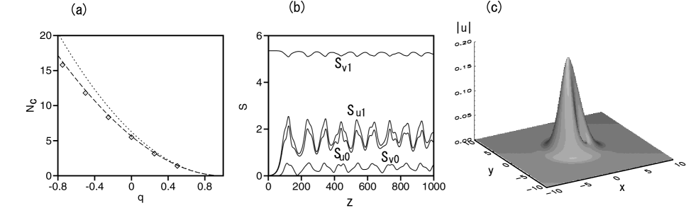
Figure 2: (a) The critical power for the onset of the parametric instability of the single-color semi-vortex with topological charge $1/2$ ($m=1$). Chains of rhombuses and the dashed and dotted curves show, respectively, numerical results and the prediction of the variational approximation produced by Eqs. (20) and (21). (b) An example of quasi-chaotic oscillations of an unstable perturbed solution is shown for $m=1,~{}q=0$, and $N=5.8$. (c) The 3D profile of the FF component of the same solution at $z=1000$.

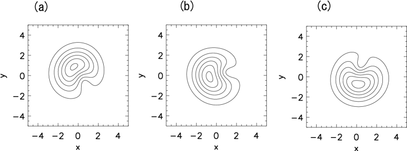
Figure 3: Contour plots of the FF component of the same solution which is displayed in Figs. 2(b,c), at $z=1000$ (a), $z=1002$ (b), and $z=1004$ (c).

IV The stability of two-color beams

While the single-color beams, with $u=0$, are unstable at $N>N_{c}^{(m)}$, in precisely the same region there appear two-color modes for $m=0$ and $m=2$ , built of the FF ($u\neq 0$) and SH fields. In other words, $N_{c}^{(m)}$ is not only the stability border for the trapped single-color modes, but also the existence threshold for their two-color counterparts. It is relevant to stress that, as seen from Fig. 1 and Eqs. (14) and (21), the threshold vanishes at $q\geq 1$.

It is easy to construct the two-color solutions for $m=0$, in the form of $u\left(x,y,z\right)=e^{-i\mu z}u_{0}(r),~{}v\left(x,y,z\right)=e^{-2i\mu z}v_{0}(r)$. These solutions exist at $N>N_{c}^{(m=0)}$ as completely stable modes, which is natural, as 2D fundamental solitons in the $\chi^{(2)}$ system are stable even in the absence of the trapping potential review1 ; review2 .

The transition from the solutions with $u=0$ to $u\neq 0$, with the simultaneous destabilization of the single-color state, is a pitchfork bifurcation, which happens with the increase of $N$, as is shown in Fig. 4 for $m=2$ (the pitchfork must give rise to two mutually symmetric modes at $N>N_{c}$, which corresponds to the obvious fact that any solution with $u\neq 0$ has its counterpart with the same $v$ and $u\rightarrow-u$). Of course, such an transition does not occur for the single-color half-vortices with $m=1$, as in that case the FF field, $u\left(x,y,z\right)\neq 0$, would carry intrinsic vorticity $m/2=1/2$, which is impossible.

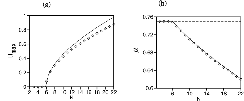
Figure 4: Amplitude $u_{\max}$ of the FF field (a) and propagation constant (b) of the solitary-vortex beams with $m=2$ at $q=0$, of both the single- and two-color types, at $N<N_{c}^{(m=2)}$ and $N>N_{c}^{(m=2)}$, respectively. The pitchfork bifurcation occurs at $N=N_{c}^{(m=2)}$. Chains of rhombuses and the dashed curve show, respectively, numerical results and the prediction of the variational approximation based on ansatz (22).

For the vortex with $m=2$, the solution extended past the bifurcation point can be looked for as per the ansatz

$$u\left(x,y,z\right)=u_{10}r\exp\left(-i\mu z+i\theta-\alpha r^{2}\right),\ v\left(x,y,z\right)=v_{20}r^{2}\exp\left(-2i\mu z+2i\theta-\beta r^{2}\right),$$ (22)

whose total power is [cf. Eq. (5)]

$$N=\pi\left[\left(2\alpha\right)^{-2}u_{10}^{2}+\beta^{-3}v_{20}^{2}\right],$$ (23)

with variational parameters $u_{10}$, $v_{20}$ and $\alpha$, $\beta$. Figure 4 shows the amplitude of $u_{10}$ and propagation constant $\mu$ for the vortex beams with $m=2$ at $q=0$, as predicted by the VA on the basis of this ansatz, and as found from numerical solutions. The dashed line in Fig. 4(b) represents the constant value, $\mu=3/4+q/2$, for the single-color vortex with $m=2$, which is unstable at $N>N_{c}^{(m=2)}$. The VA is very accurate close to the bifurcation point, showing a discrepancy which slowly increases at large $N$.

A crucially important issue is the stability of the vortex beams at $N>N_{c}^{(m=2)}$, as all such states are unstable against azimuthal splitting in the free space splitting1 -splitting-exp . In the analytical form, the stability can be explored by mean of the nonstationary version of the VA, based on the following ansatz, which adds perturbations containing spatial harmonics with numbers $-1$ and $3$ in the FF field, and zeroth and fourth harmonics in the SH component, to the stationary solution taken as per Eq. (22) (such perturbations induce the splitting instability of the solitary vortex in the free space):

$$u\left(x,y,z\right) = u_{1}(z)r\exp\left(i\theta-\alpha r^{2}\right)+u_{-1}(z)r\exp\left(-i\theta-\alpha_{-1}r^{2}\right)+u_{3}(z)r^{3}\exp\left(3i\theta-\alpha_{3}r^{2}\right),$$

$$v\left(x,y,z\right) = v_{2}(z)r^{2}\exp\left(2i\theta-\beta r^{2}\right)+v_{0}(z)\exp\left(-\beta_{0}r^{2}\right)+v_{4}(z)r^{4}\exp\left(4i\theta-\beta_{4}r^{2}\right).$$ (24)

Here $\alpha$ and $\beta$ are the same as found from the stationary version of the VA based on ansatz (22). Straightforward calculations lead to the following linearized evolution equations for the perturbation amplitudes:

$$i\frac{du_{-1}}{dz} = \left(2\alpha_{-1}+\frac{1}{8\alpha_{-1}}\right)u_{-1}-\frac{4\alpha_{-1}u_{1}^{\ast}v_{0}}{(\alpha+\alpha_{-1}+\beta_{0})^{2}}-\frac{24\alpha_{-1}^{2}u_{3}^{\ast}v_{2}}{(\alpha_{-1}+\alpha_{3}+\beta)^{4}},$$

$$i\frac{du_{3}}{dz} = \left(4\alpha_{3}+\frac{1}{4\alpha_{3}}\right)u_{3}-\frac{16\alpha_{3}^{4}u_{-1}^{\ast}v_{2}}{(\alpha_{-1}+\alpha_{3}+\beta)^{4}}-\frac{64\alpha_{3}^{4}u_{1}^{\ast}v_{4}}{(\alpha+\alpha_{3}+\beta_{4})^{4}},$$

$$i\frac{dv_{0}}{dz} = \left[\beta_{0}+\frac{1}{2\left(4\beta_{0}+q\right)}\right]v_{0}-\frac{\beta_{0}u_{1}u_{-1}}{(\alpha+\alpha_{-1}+\beta_{0})^{2}},$$

$$i\frac{dv_{4}}{dz} = \left[\frac{5\beta_{4}}{2}+\frac{1}{2\left(4\beta_{4}+q\right)}\right]v_{4}-\frac{16\beta_{4}^{5}u_{1}u_{3}}{(\alpha+\alpha_{3}+\beta_{4})^{5}}.$$ (25)

Solutions to Eqs. (25) are looked for as $u_{-1}=u_{-1}^{(0)}e^{-i\gamma_{-1}z},u_{3}=u_{3}^{(0)}e^{-i\gamma_{3}z},v_{0}=v_{0}^{(0)}e^{-i\gamma_{0}z}$, $v_{4}=v_{4}^{(0)}e^{-i\gamma_{4}z}$, with propagation constants subject to the matching conditions, which ensue from the substitution of expressions (22) into Eqs. (25):

$$\gamma_{0}=\mu+\gamma_{-1},\gamma_{3}=2\mu-\gamma_{-1},\gamma_{4}=3\mu-\gamma_{-1}.$$ (26)

Finally, the eigenvalue problem for $\gamma_{-1}$ amounts to the following equation, in which $\gamma_{0}$, $\gamma_{3}$, and $\gamma_{4}$ should be substituted as per Eq. (26):

$$\frac{6\alpha_{-1}^{2}\alpha_{3}^{4}\left(8v_{20}\right)^{2}}{(\alpha_{-1}+\alpha_{3}+\beta)^{8}}=\left[2\alpha_{-1}+\frac{1}{8\alpha_{-1}}-\gamma_{-1}-\frac{32\alpha_{-1}^{2}\beta_{0}u_{10}^{2}}{(\alpha+\alpha_{-1}+\beta_{0})^{4}(4\beta_{0}+\beta_{0}^{-1}+4q-8\gamma_{0})}\right]$$

$$\times\left[4\alpha_{3}+\frac{1}{4\alpha_{3}}-\gamma_{3}-\frac{2\alpha_{3}^{4}\beta_{4}^{5}\left(64u_{10}\right)^{2}}{(\alpha+\alpha_{3}+\beta_{4})^{10}(20\beta_{4}+5\beta_{4}^{-1}+4q-8\gamma_{4})}\right].$$ (27)

The critical value of the total power [see Eq. (23)] at the onset of the instability of the trapped vortex (22), $N=N_{c2}$, is identified as the one at which eigenvalue $\gamma_{-1}$, found from Eq. (27), becomes complex. Then, it should be minimized by varying the set of parameters $\alpha_{-1},\alpha_{3},\beta_{0}$ and $\beta_{3}$, cf. Eqs. (10), (13), and (20). Actually, this procedure is too cumbersome in its full form, but we have found that a nearly-minimum value of $N_{c2}$ corresponds to $\alpha_{-1}=\alpha_{3}=1.2\alpha$ and $\beta_{0}=\beta_{3}=0.5$. The result is reported in Fig. 5(a), which displays $N_{c2}$ versus $q$, along with the previously found critical value, $N_{c}$, which is the border between the stable single-color vortices and emerging stable two-color ones. As seen from the figure, the two-color vortex is completely unstable at $q<q_{\min}\approx-0.5$, and has an expanding stability area at $q>q_{\min}$. The increase of $N_{c2}$ with mismatch $q$ is explained by the fact that large $q$ corresponds to the cascading limit review0 -review2 , in which the $\chi^{(2)}$ nonlinearity is transformed into the self-focusing cubic interaction, with a decreasing effective cubic coefficient, $\chi^{(3)}\sim 1/q$, and the vortices trapped by the HO potential in the respective weakly nonlinear cubic medium have a large stability area cubic-in-trap1 -cubic-in-trap7 . The accuracy of the VA prediction for $N_{c2}$ is essentially lower than it was for $N_{c}$, because the variational ansätze (22) and (24) cannot approximate the complex structure of the respective modes accurately enough, and by the above-mentioned fact that the full minimization procedure is too cumbersome in this case [in particular, we expect that a more thorough procedure would make the VA-predicted values of $N_{c2}$ somewhat smaller than those plotted in Fig. 5(a), thus reducing the discrepancy with the numerically found stability border]. Nevertheless, the VA predicts the value of $q=q_{\min}$ almost exactly, and the general shape of the stability boundary, $N=N_{c2}(q)$, is predicted correctly too.

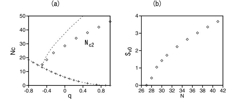
Figure 5: (a) The stability area of the two-color vortices with topological charge $1$ ($m=2$), in the plane of the mismatch ($q$) and total power ($N$), is $N_{c}<N<N_{c2}$. The numerically found stability borders and their counterparts predicted by the variational approximation are displayed by chains of symbols and dashed lines, respectively [in fact, $N_{c}(q)$ is the same border as one labeled by $m=2$ in Fig. 1(a)]. (b) The peak value of the integral amplitude of the zeroth angular harmonic of the SH field, $S_{v0}(z)$ [defined as per Eq. (15)], as found from the simulations of the oscillatory solutions at $N>N_{2c}\approx 27.5$ for $q=0$.

At $N>N_{c2}$, the simulations demonstrate that the instability transforms the stationary two-color vortex into a persistent oscillatory one, which keeps the vortical component, mixing it with the zero-vorticity one. To illustrate this finding, the peak values (largest over the period of the oscillations) of the integrally defined amplitude of the zeroth angular component in the SH field, $S_{v0}(z)$ [see Eq. (15)], is displayed as a function of $N$ in Fig. 5(b) for $q=0$. The persistent oscillatory dynamics developed by the unstable two-color vortices at $N>N_{c2}$ is further illustrated in Fig. 6 by the evolution of the integrated amplitudes $S_{u1}(z)\$and $S_{v0}(z)$ [defined as per Eqs. (16) and (15)], produced by the direct simulations for $q=0$ and $N=39$, cf. Fig. 1(c) for unstable single-color vortices. In particular, Fig. 6(a) implies that the oscillating mode keeps its vorticity.

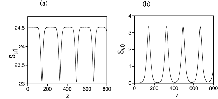
Figure 6: The periodic evolution of the integrally defined amplitudes of the first angular harmonic in the FF field (a), and the zeroth harmonic in the SH field (b).

In fact, the oscillating vortices undergo periodic splitting and recoveries. An example of this generic dynamical regime as shown in Fig. 7 for the same mode whose evolution is presented in Fig. 6. A similar persistent regime was found in the 2D model with the self-attractive cubic nonlinearity, above the threshold of the instability of trapped vortices (see details in Ref. cubic-in-trap5 ). However, in the case of the cubic equation the splitting-recovery scenario is replaced, at still larger $N$, by the onset of the collapse, which does not occur in the $\chi^{(2)}$ system.

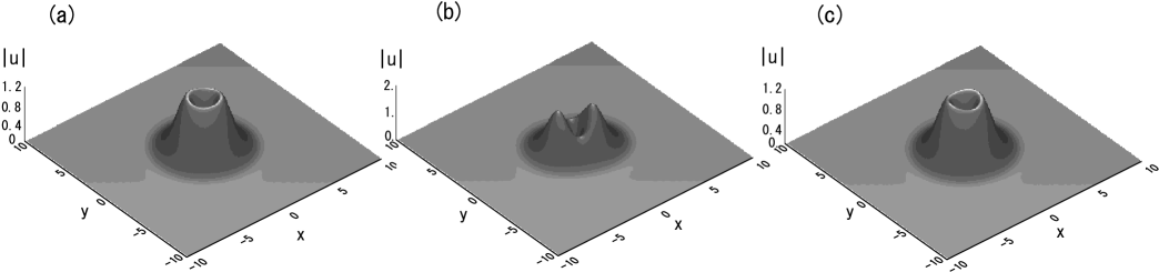
Figure 7: The regime of periodic splittings and recoveries of an unstable two-color vortex (the same one whose evolution is presented in Fig. 6) is illustrated by a sequence of profiles of $\left|u\left(x,y,z\right)\right|$ at $z=90$ (a), $140$ (b), and $190$ (c).

V Conclusion

The objective of this work is to demonstrate the possibility of the stabilization of $\chi^{(2)}$ solitary-vortex modes by the isotropic trapping potential. The existence and stability of various modes supported by the system is determined by the total power, $N$, mismatch $q$, and modal topological charge, $m/2$ ($m$ is the intrinsic vorticity of the SH component). Using, in parallel, numerical solutions and static and dynamical versions of the VA (variational approximation), we have found that, at $N<N_{c}^{(m)}(q)$, all modes are of the single-color type, represented by the SH (second-harmonic) component only. In contrast with the usual assumption that such modes are subject to the parametric instability against the generation of the FF (fundamental-frequency) field, we have demonstrated that they are stable at $N<N_{c}^{(m)}(q)$, including the (formal) semi-vortex with topological charge $1/2$ ($m=1$). However, $N_{c}^{(m)}(q)\equiv 0$ at $q>1$, i.e., the single-color modes are indeed completely unstable at large $q$. The modes with $m=0$ and $m=2$ undergo pitchfork bifurcations exactly at $N=N_{c}^{(m)}$, which, destabilizing the single-color states, give rise to stable two-color complexes. For $m=0$, the emerging states are always stable, while the vortical two-color mode, with $m=2$, has an upper stability limit, $N=N_{c2}(q)$. At $N>N_{c2}(q)$, the unstable vortices feature periodic splittings and recoveries, keeping their topological charge. In addition to optics, these results may be realized in atomic-molecular BEC mixtures. The semi-vortex does not bifurcate at $N=N_{c}^{(m=1)}$; instead, it develops persistent quasi-chaotic oscillations, involving additional angular harmonics in both the SH and FF fields, and features a rotating “groove”, which resembles the mixed screw-edge dislocation induced by the semi-integer vorticity.

This work suggests possibilities for the analysis in other directions. The stability of trapped vortices and semi-vortices with higher values of the topological charge ($m/2=1.5,~{}2,~{}2.5,~{}3,...$) may be a natural generalization, as well as the consideration of trapped modes in the framework of the Type-II (three-wave) $\chi^{(2)}$ system. On the other hand, it may be easy to perform a similar analysis for fundamental and higher-order odd and even (spatially antisymmetric and symmetric, respectively) modes in the 1D version of the $\chi^{(2)}$ system. In particular, the trapping potential may have a chance to stabilize the 1D odd modes, which are always unstable in the free space Werner . On the other hand, a challenging problem is to find stable solutions for 3D “bullets” in the extended version of system (1), including the temporal variable and group-velocity-dispersion terms. The possibility of the existence of stable “bullets” with embedded vorticity is an especially intriguing issue (cf. Ref. 3Dvortex , where stable “spinning bullets” were found in the free-space model combining the $\chi^{(2)}$ and self-defocusing $\chi^{(3)}$ nonlinearities). The 3D setting makes it also possible to study collisions between stable solitons moving along the trapping potential pipe.

References

- (1) G. I. Stegeman, D. J. Hagan, and L. Torner, “ cascading phenomena and their applications to all-optical signal processing, mode-locking, pulse compression and solitons”, Opt. Quant. Electr. 28, 1691-1740 (1996).
- (2) C. Etrich, F. Lederer, B. A. Malomed, T. Peschel, and U. Peschel, “Optical solitons in media with a quadratic nonlinearity”, Progr. Opt. 41, 483-568 (2000).
- (3) A. V. Buryak, P. Di Trapani, D. V. Skryabin, and S. Trillo, “Optical solitons due to quadratic nonlinearities: from basic physics to futuristic applications”, Phys. Rep. 370, 63-235 (2002).
- (4) B. A. Malomed, D. Mihalache, F. Wise, and L. Torner, “Spatiotemporal optical solitons”, J. Optics B: Quant. Semicl. Opt. 7, R53-R72 (2005).
- (5) Y. S. Kivshar and G. P. Agrawal, Optical Solitons: From Fibers to Photonic Crystals (San Diego, CA: Academic, 2003).
- (6) F. Du, Y. W. Lu, and S. T. Wu, “Electrically tunable liquid-crystal photonic crystal fiber”, Appl. Phys. Lett. 85, 2181-2183 (2004).
- (7) F. Luan, A. K. George, T. D. Hedeley, G. J. Pearce, D. M. Bird, J. C. Knight, and P. S. J. Russell, “All-solid photonic bandgap fiber,” Opt. Lett. 29, 2369-2371 (2004).
- (8) A. A. Kanashov and A. M. Rubenchik, “On diffraction and dispersion effect on three wave interaction”, Physica D 4, 122-134 (1981).
- (9) W. E. Torruellas, Z. Wang, D. J. Hagan, E. W. VanStryland, G. I. Stegeman, L. Torner, and C. R. Menyuk, “Observation of Two-Dimensional Spatial Solitary Waves in a Quadratic Medium”, Phys. Rev. Lett. 74, 5036-5039 (1995).
- (10) B. A. Malomed, P. Drummond, H. He, A. Berntson, D. Anderson, and M. Lisak, “Spatiotemporal solitons in multidimensional optical media with a quadratic nonlinearity”, Phys. Rev. E 56, 4725-4735 (1997).
- (11) X. Liu, L. J. Qian, and F. W. Wise, “Generation of optical spatiotemporal solitons”, Phys. Rev. Lett. 82, 4631-4634 (1999).
- (12) X. Liu, K. Beckwitt, and F. Wise, “Two-dimensional optical spatiotemporal solitons in quadratic media”, Phys. Rev. E 62, 1328-1340 (2000).
- (13) F. A. Bovino, M. Braccini, and C. Sibilia, “Orbital angular momentum in noncollinear second-harmonic generation by off-axis vortex beams”, J. Opt. Soc. A, B 28, 2806-2811 (2011).
- (14) W. J. Firth and D. V. Skryabin, “Optical solitons carrying orbital angular momentum”, Phys. Rev. Lett. 79, 2450-2453 (1997).
- (15) L. Torner and D. V. Petrov, “Azimuthal instabilities and self-breaking of beams into sets of solitons in bulk second-harmonic generation”, Electron. Lett. 33, 608-610 (1997).
- (16) D. V. Skryabin and W. J. Firth, “Instabilities of higher-order parametric solitons: Filamentation versus coalescence”, Phys. Rev. E 58, R1252-R1255 (1998).
- (17) J. P. Torres, J. M. Soto-Crespo, L. Torner, and D. V. Petrov, “Solitary-wave vortices in quadratic nonlinear media”, J. Opt. Soc. Am. B 15, 625-627 (1998).
- (18) D. V. Petrov, L. Torner, J. Martorell, R. Vilaseca, J. P. Torres, and C. Cojocaru, “Observation of azimuthal modulational instability and formation of patterns of optical solitons in a quadratic nonlinear crystal”, Opt. Lett. 23, 1444-1446 (1998).
- (19) J. P. Torres, J. M. Soto-Crespo, L. Torner, and D. V. Petrov, “Solitary-wave vortices in type II second-harmonic generation”, Opt. Commun. 149, 77-83 (1998).
- (20) G. Molina-Terriza, E. M. Wright, and L. Torner, “Propagation and control of noncanonical optical vortices”, Opt. Lett. 26, 163-165 (2001).
- (21) V. I. Kruglov, Y. A. Logvin, and V. M. Volkov, “The theory of spiral laser-beams in nonlinear media”, J. Mod. Opt. 39, 2277-2291 (1992).
- (22) C. J. Pethick and H. Smith, Bose-Einstein condensate in dilute gas (Cambridge University Press: Cambridge, 2008).
- (23) F. Dalfovo and S. Stringari, “Bosons in anisotropic traps: Ground state and vortices”, Phys. Rev. A 53, 2477-2485 (1996).
- (24) R. J. Dodd, “Approximate solutions of the nonlinear Schrödinger equation for ground and excited states of Bose-Einstein condensates”, J. Res. Natl. Inst. Stand. Technol. 101, 545-552 (1996).
- (25) T. J. Alexander and L. Bergé, “Ground states and vortices of matter-wave condensates and optical guided waves”, Phys. Rev. E 65, 026611 (2002).
- (26) L. D. Carr and C. W. Clark, “Vortices in attractive Bose-Einstein condensates in two dimensions”, Phys. Rev. Lett. 97, 010403 (2006).
- (27) D. Mihalache, D. Mazilu, B. A. Malomed, and F. Lederer, “Vortex stability in nearly-two-dimensional Bose-Einstein condensates with attraction”, Phys. Rev. A 73, 043615 (2006).
- (28) L. D. Carr and C. W. Clark, “Vortices and ring solitons in Bose-Einstein condensates”, Phys. Rev. A 74, 043613 (2006).
- (29) G. Herring, L. D. Carr, R. Carretero-González, P. G. Kevrekidis, and D. J. Frantzeskakis, “Radially symmetric nonlinear states of harmonically trapped Bose-Einstein condensates”, Phys. Rev. A 77, 043607 (2008).
- (30) P. D. Drummond, K. V. Kheruntsyan, and H. He, “Coherent molecular solitons in Bose-Einstein condensates”, Phys. Rev. Lett. 81, 3055-3058 (1998).
- (31) D. J. Heinzen, R. Wynar, P. D. Drummond, and K. V. Kheruntsyan, “Superchemistry: Dynamics of coupled atomic and molecular Bose-Einstein condensates”, Phys. Rev. Lett. 84, 5029-5033 (2000).
- (32) J. J. Hope and M. K. Olsen, “Quantum superchemistry: Dynamical quantum effects in coupled atomic and molecular Bose-Einstein condensates”, Phys. Rev. Lett. 86, 3220-3223 (2001).
- (33) T. Hornung, S. Gordienko, R. de Vivie-Riedle, and B. J. Verhaar, “Optimal conversion of an atomic to a molecular Bose-Einstein condensate”, Phys. Rev. A 66, 043607 (2002).
- (34) Z. Y. Xu, Y. V. Kartashov, L. C. Crasovan, D. Mihalache, and L. Torner, “Multicolor vortex solitons in two-dimensional photonic lattices”, Phys. Rev. E 71, 016616 (2005).
- (35) M. J. Werner and P. D. Drummond, “Strongly coupled nonlinear parametric solitary waves”, Opt. Lett. 19, 613-615 (1994).
- (36) D. Mihalache, D. Mazilu, L. C. Crasovan, I. Towers, B. A. Malomed, A. V. Buryak, L. Torner, and F. Lederer, “Stable three-dimensional spinning optical solitons supported by competing quadratic and cubic nonlinearities”, Phys. Rev. E 66, 016613 (2002).