Pyrochlore electrons under pressure, heat and field: shedding light on the iridates

Abstract

We study the finite temperature and magnetic field phase diagram of electrons on the pyrochlore lattice subject to a local repulsion as a model for the pyrochlore iridates. We provide the most general symmetry-allowed Hamiltonian, including next-nearest neighbour hopping, and relate it to a Slater-Koster based Hamiltonian for the iridates. It captures Lifshitz and/or thermal transitions between several phases such as metals, semimetals, topological insulators and Weyl semimetals, and gapped antiferromagnets with different orders. Our results on the charge conductivity, both DC and optical, Hall coefficient, magnetization and susceptibility show good agreement with recent experiments and provide new predictions. As such, our effective model sheds light on the pyrochlore iridates in a unified way.

I Introduction

The pyrochlore iridates, R₂Ir₂O₇ (R-227) where R is a rare earth, provide an ideal setup to study the interplay of correlations, band topology and frustration. Building in part on the strong role of spin-orbit coupling (SOC) and correlations for IrKim et al. (2008); *SrIrO-science, various novel phases have been predicted to potentially occur in this family of complex oxides such as fractionalized topological insulatorsPesin and Balents (2010); Witczak-Krempa et al. (2010) (TIs), chiral spin liquidsMachida et al. (2009), topological Weyl semimetalsWan et al. (2011); Witczak-Krempa and Kim (2012) (TWSs), and axion insulatorsGo et al. (2012); Wan et al. (2011). This has contributed to a substantial experimental effortYanagishima and Maeno (2001); Taira et al. (2001); Fukazawa and Maeno (2002); Matsuhira et al. (2007, 2011); Hasegawa et al. (2010); Zhao et al. (2011); Ishikawa et al. (2012); Tomiyasu et al. (2012); Tafti et al. (2012); Sakata et al. (2011); Shapiro et al. (2012); Disseler et al. (2012a, b), in particular to determine the nature of the still-elusive magnetic ordering, except for Pr-227 which shows no sign of long-range order down to the lowest accessible temperatures. Recent theoretical and experimental work has been pointing towards a $q=0$ all-in/all-out (AIO) magnetic pattern in the ground stateWan et al. (2011); Witczak-Krempa and Kim (2012); Zhao et al. (2011); Ishikawa et al. (2012); Tomiyasu et al. (2012); Disseler et al. (2012a, b) but direct evidence is still lacking. Another question concerns the nature of the metal insulator transition as a function of chemical pressure via the change of the R-site elementYanagishima and Maeno (2001); Matsuhira et al. (2007, 2011) or hydrostatic pressureTafti et al. (2012); Sakata et al. (2011), as well as the nature of the thermal continuous transitions: what are the respective roles of magnetic ordering, Mott physics, and band structure? Finally, are any of the new phases, for example the TWS, present in the actual compounds?

We provide insight into these questions by considering a microscopically-motivated Hubbard model which we probe at finite temperature and magnetic field. We compute transport, magnetization and susceptibility in the various phases (metal (M), TI, TWS, AIO, antiferromagnet (AF), etc) as well as their behaviour across the phase transitions, quantum or thermal. The similarity of our results with recent experimental data allows us to make guesses on the locations of different iridates in our phase diagram, and make predictions for future experiments. Before considering the observables, we discuss a fully general Hubbard Hamiltonian on the pyrochlore lattice, its relation to previous models used for the iridates, and to the new model underlying this work.

The iridium ions form a pyrochlore lattice of corner-sharing tetrahedra and have a partially filled shell of 5d electrons. This results in the local repulsion and spin orbit coupling being of similar size, both on the order of 0.5-1 eVPesin and Balents (2010); Wan et al. (2011). The localized f-electrons of the R-site (absent for Y) can complicate the picture for some members of the iridates family for which the R-site ion carries a net magnetic moment. In this work we shall not consider the interplay between these local moments and the more itinerant Ir d-electrons. As such, our results apply directly to the compounds with Y, Lu and Eu for which this complication does not arise. Regarding the compounds with a magnetic R-site, such as for $R=$ Nd, Sm, Yb, etc, the Ir d-electron physics might still play a key role. Indeed, the similarity of the phenomena across the pyrochlore iridates family, independent of whether the R-site is magnetic or not, provide weight to this statementYanagishima and Maeno (2001); Taira et al. (2001); Matsuhira et al. (2007, 2011); Hasegawa et al. (2010); Disseler et al. (2012b). In the context of the pyrochlore iridates, a recent workChen and Hermele (2012) has examined the interplay between the more itinerant $d$-electrons and the localized $f$-electron moments by including an exchange coupling between our nearest neighbor hopping HamiltonianWitczak-Krempa and Kim (2012), Eq. (1), and an appropriate spin model. It was found that Weyl semimetal and axion insulatorWan et al. (2011); Go et al. (2012) phases can be induced by the $f-d$ exchange, and that the latter can cooperate with the Hubbard interaction on Ir sites to stabilize the Weyl semimetal over a larger region of parameter space than when it is induced by $d$-electron correlations alone. Further studies in that direction will be of interest, notably to get a better understanding of the chiral spin liquid behavior of Pr-227Machida et al. (2009).

The outline is as follows: we first introduce the general Hamiltonian in Section II and relate it to previous works. The ground state phase diagram and its extension to finite temperature is obtained in Section III. The conductivities, both d.c. and optical, are then discussed in Section IV. We discuss the finite-magnetic field phase diagram in Section V. Finally, we briefly summarize in Section VI and draw connections between our results and experiments on the pyrochlore iridates.

II Model demystified

Rather than starting with a specific microscopic model for the iridates, we consider the most generic, time-reversal invariant Hubbard Hamiltonian on the pyrochlore lattice. We shall focus on an effective model with a single Kramers’ doublet at each Ir site. This will lead to an 8-band model that we believe is sufficient to capture the salient physics. We write the Hamiltonian in a global basis for the pseudospin to emphasize its simplicity and generality:

$$H_{0}=\sum_{\begin{subarray}{c}\langle i,j\rangle\end{subarray}}c_{i}^{\dagger}(t_{1}+it_{2}{\bm{d}}_{ij}\cdot{\bm{\sigma}})c_{j}\\ +\sum_{\begin{subarray}{c}\langle\langle i,j\rangle\rangle\end{subarray}}c_{i}^{\dagger}(t_{1}^{\prime}+i[t_{2}^{\prime}\bm{\mathcal{R}}_{ij}+t_{3}^{\prime}\bm{\mathcal{D}}_{ij}]\cdot{\bm{\sigma}})c_{j}\,,$$ (1)

where ${\bm{\sigma}}$ is a vector of Pauli matrices acting on the pseudospin degree of freedom, which in the context of the iridates can be thought of as arising from the splitting of the $t_{2g}$ levels by SOCKim et al. (2008); *SrIrO-science and/or trigonal distortionsYang and Kim (2010); Kargarian et al. (2011) and subsequent projection onto a half-filled doublet near the Fermi level ($E_{F}$). The real vectors ${\bm{d}}_{ij},\bm{\mathcal{R}}_{ij},\bm{\mathcal{D}}_{ij}$ depend on the given bond as follows: ${\bm{d}}_{ij}$ is aligned along the opposite bond of the tetrahedron containing $i,j$ (Fig. 8); it is parallel or antiparallel with the nearest neighbor (NN) Dzyaloshinski-Morya (DM) vector of a spin model on the pyrochlore lattice, of which there are only two symmetry-allowed configurationsElhajal et al. (2005); Witczak-Krempa and Kim (2012), differing by a global sign. $\bm{\mathcal{R}}_{ij},\bm{\mathcal{D}}_{ij}$ are obtained by going to the next nearest neighbour (NNN) via the common NN site and taking a cross product of the two bond or ${\bm{d}}_{ij}$ vectors encountered, respectively. See Appendix A for details regarding the construction of Eq. (1). The five real hopping amplitudes lead to a four-parameter free model, to which we add a Hubbard repulsion term, $H_{U}=(U/2)\sum_{i}(n_{i}-1)^{2}$. In this work we perform a mean field decoupling of $H_{U}$ in the magnetic channel, but expect many results to survive the inclusion of quantum many-body effects. Indeed, a subset of many-body effects was taken into account in our recent studyGo et al. (2012) of the NN Hamiltonian using cellular dynamical mean-field theory (CDMFT). For instance, we obtained the same magnetic orders as those found at the mean-field field level.

Figure 1: Phase diagram of the generic NN hopping Hamiltonian on a pyrochlore lattice. It has two possible phases: a TI and a SM. The square indicates the presence of a gap closing, surrounded by the TI phase.

Before discussing the relation of Eq. (1) to previous microscopic models for the iridates and to the one used in this work, we briefly discuss the phase diagram including only NN hopping. It depends on a single parameter, $t_{2}/t_{1}$, and can be determined exactly at half-filling; the result is shown in Fig. 1. For $-2<t_{2}/t_{1}<0$ a semimetal (SM) results, and otherwise we have a TIMoore and Balents (2007); *roy; *fu-kane-mele, with the exception of $t_{2}/t_{1}=1$ where an accidental gap closing occurs. Interestingly, it does not alter the topological structure of the Hamiltonian such that the TI survives to arbitrary large values of $t_{2}/t_{1}$. The SM is characterized by lines of nodes between the $\Gamma$ and $L$ points. The phase transitions at $t_{2}/t_{1}=-2,0$ occur via gap closing/opening at the $\Gamma$ point. At $t_{2}=0$, the Hamiltonian can be diagonalized analyticallyGuo and Franz (2009). Interestingly, it is also the case at $t_{2}/t_{1}=-2$, where the band structure corresponds exactly to the $t_{2}=0$ case, albeit with a spectrum inversion; specifically: $\{t_{1}=1,t_{2}=-2\}$ maps to $\{-3,0\}$. The phase transition at $t_{2}/t_{1}=0$ was previously discussedKurita et al. (2011), where the $t_{1,2}$ model was identified as the most general NN symmetry-allowed Hamiltonian.

We now relate the general parameters to microscopically-motivated ones for the iridates. We first consider the case of no trigonal distortionPesin and Balents (2010); Witczak-Krempa and Kim (2012), leading to ideal oxygen octahedra surrounding the iridiums. The SOC splits the $t_{2g}$ manifold into $J_{\rm eff}=1/2$ and $3/2$ multiplets. Projecting onto the half-filled doublet near $E_{F}$ yields a pseudospin $J_{\rm eff}=1/2$ description. Going from the atomic picture to the lattice, we introduce oxygen-mediatedPesin and Balents (2010) and directWitczak-Krempa and Kim (2012) overlap NN hopping $t_{\rm oxy}$ and $t_{\sigma},t_{\pi}$, respectively. These relate to the generic model hoppings via:

$$t_{1} =\frac{130t_{\rm oxy}}{243}+\frac{17t_{\sigma}}{324}-\frac{79t_{\pi}}{243};\quad\,\,t_{1}^{\prime}=\frac{233t_{\sigma}^{\prime}}{2916}-\frac{407t_{\pi}^{\prime}}{2187}\,;$$

$$t_{2} =\frac{28t_{\rm oxy}}{243}+\frac{15t_{\sigma}}{243}-\frac{40t_{\pi}}{243};\,\;\;\;\;\quad t_{2}^{\prime}=\frac{t_{\sigma}^{\prime}}{1458}+\frac{220t_{\pi}^{\prime}}{2187}\,;$$

$$t_{3}^{\prime} =\frac{25t_{\sigma}^{\prime}}{1458}+\frac{460t_{\pi}^{\prime}}{2187}\,;$$ (2)

where we have also added $t_{\sigma,\pi}^{\prime}$, the $\sigma$- and $\pi$-overlap NNN hoppings. We see that the microscopic model already saturates the general Hamiltonian. As such, small trigonal distortionsYang and Kim (2010) will renormalize the $t_{a}^{(\prime)}$ but will not contribute new terms allowing us to use the $J_{\rm eff}=1/2$ description without loss of generality. We mention that Ref. Pesin and Balents, 2010 used purely oxygen mediated hopping, hence their large SOC TI can be mapped to $t_{2}/t_{1}=14/65\approx 0.215$ which indeed corresponds to a TI in Fig. 1. Also, Ref. Guo and Franz, 2009 studied TIs in the $t_{1},t_{2}^{\prime}$ model.

We shall work in units of $t_{\rm oxy}$ in the rest of the paper. As before, we choose a representative subset of direct hoppings, $t_{\pi}=-2t_{\sigma}/3$, which translates to $t_{1}=0.53+0.27t_{\sigma}$ and $t_{2}=0.12+0.17t_{\sigma}$. We plot the relation between $t_{2}/t_{1}$ and $t_{\sigma}/t_{\rm oxy}$ in Fig. 9. An important addition in this work is the presence of small NNN hoppings: $t_{\sigma}^{\prime}/t_{\sigma}=t_{\pi}^{\prime}/t_{\pi}=0.08$. These are expected to appear in the effective pseudospin model, and will remove line Fermi surfaces at $E_{F}$ in some portions of the phase diagram, giving instead a TWS or metal with small pocketsWitczak-Krempa and Kim (2012). The line nodes are an artifact of the NN band structure.

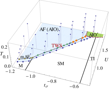
Figure 2: Finite $U$ & $T$ mean field phase diagram, including small NNN hopping ($t_{\rm oxy}=1$). The out-of-plane fibers give $T_{c}$ for the continuous transition at which the magnetic order melts. The two shaded regions correspond to AF phases: either the AIO AF, or a type related by $\pi/2$ rotations, AIO^′. The solid/dashed lines denote 2nd/1st order quantum phase transitions, while the dotted lines in the AIO phase, a gap closing signaling a Lifshitz transition out of the TWS or metallic AF (mAF).

III Phase diagram

The mean field phase diagram is shown in Fig. 2. At $T=0$ and small $U$, it contains metallic (M), SM and TI phases depending on $t_{\sigma}$. The metallic state has electron- and hole-like pockets while the SM is associated with a quadratic band touching, that splits into 8 linearly dispersing touchings in the AF TWSWitczak-Krempa and Kim (2012), see the spectra in Fig. 3(b) or in Fig. 5 c). The shaded regions break TRS due to the appearance of either the symmetric AIO order (pale blue), or orders which are related to the AIO state by local $\pi/2$ rotationsWitczak-Krempa and Kim (2012) (denoted by AIO^′, in green). At intermediate $U$, there is an extended region of TWS, which turns into a metallic AF (mAF) for $t_{\sigma}<-1.085$. The latter is actually a tilted TWS, where the 3D “Dirac cones” have been tilted such as to create metallic pockets, but with the “Weyl touchings” remaining, see Fig. 3(a). These phases should be compared with similar results obtained in Ref. Witczak-Krempa and Kim (2012) by two of us. The main difference is that we have now included the NNN hoppings in the self-consistent treatment. Indeed, the previous work was mainly concerned with the self-consistent analysis of the NN Hamiltonian: the NNN hoppings were added to the final spectrum to establish that the line-nodes at $E_{F}$ can give rise to a Weyl phase when the ordering is of the AIO type. The present work confirms this. Moreover, a metallic phase now appears for $t_{\sigma}<-1.085$, which will be relevant when we compare with experiments on the iridates. Another new feature is the presence of magnetization “jumps” that appear within the AIO phase, present for $-0.78<t_{\sigma}<-0.68$, denoted by the orange (larger) markers in Fig. 2. The spontaneous onsite magnetization, $m$, grows abruptly along that line and the TWS becomes a gapped AF insulator: energetically, the system finds it preferable to preempt the continuous annihilation of Weyl points of opposite chirality via a discontinuous evolution of $m$, this is illustrated in Fig. 4. The abrupt continuous increase of magnetization seems tied to the peculiar spectrum of the TWS.

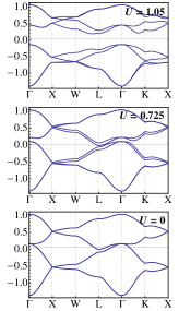
(a)  $t_{\sigma}=-1.2$

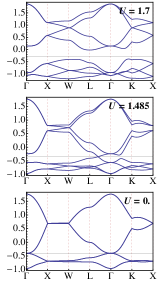
(b)  $t_{\sigma}=-0.8$

Figure 3: Spectra for the Hamiltonian Eq. (1) for (a) $t_{\sigma}=-1.2$ and (b) $t_{\sigma}=-0.8$. These are associated with the phase diagram Fig. 2.

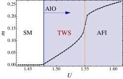
Figure 4: Evolution of the magnetization, $m$, as a function of the Hubbard repulsion $U$ for $t_{\sigma}=-0.775$. Note the abrupt evolution of $m$ when going from the TWS to the AF insulator (AFI). The shaded regions have the AIO order.

Turning to finite temperature, we find that most thermal transitions are continuous; this is denoted by the out-of-plane fibers ended by circular markers in Fig. 2. We have also examined the model at larger NNN hoppings, $t_{\sigma,\pi}^{\prime}/t_{\sigma,\pi}=0.16$, and found that small regions of 1st order transitions to the AIO phase appear at intermediate $U$. As can be seen in Fig. 2, the transition temperatures naturally increase with $U$, since an increase in the latter leads to larger gaps. Thus, the gapless TWS is fairly unstable to melting at finite $T$, with typical transition temperatures $T_{c}\sim 0.01$ in units of $t_{\rm oxy}$. We note that the continuous transitions are consistent with experimental data on the pyrochlore iridates.

IV Conductivities

IV.1 Optical conductivity

We examine the optical conductivity associated with the various phases, as illustrated in Fig. 5. Panel a) shows the Lifshitz transition associated with a change in the Fermi surface topology from a metal with small electron- and hole-like pockets at $U=0$ to a gapped AIO state at $U=1$. The optical conductivity in panel b) reflects this via a small Drude peak in the former case, and a gap in the latter. Panel c) shows the spectra of the TWS and quadratic band touching SM out of which it arose. The associated conductivities are reduced approaching the DC limit because these two states have a vanishing density of states (DOS) at $E_{F}$. We note the distinguishing peak at low frequency for the TWS: it receives weight from transitions across the depleted energy range corresponding to the TWS, where the DOS vanishes quadratically.

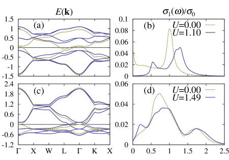
Figure 5: Spectra and corresponding optical conductivity (real part) for $t_{\sigma}=-1.2$, a) & b), and $t_{\sigma}=-0.8$, c) & d), respectively. Panel a) shows the energy spectrum ($E_{F}=0$) for the M and AIO insulator, while c) for the SM and TWS. The conductivity is in units of $\sigma_{0}=e^{2}/\hbar a_{0}\sim 10^{4}\,({\rm\Omega\cdot cm})^{-1}$, where $a_{0}=a/4$ and $a\approx 1.0$ nm is the FCC lattice constant.

IV.2 DC transport

We turn to the DC electric transport, which provides further insight into the phase diagram. The AIO state has isotropic conductivities due to the highly symmetric magnetic configuration, i.e. $\sigma_{xx}=\sigma_{yy}=\sigma_{zz}$. The same holds for the Hall conductivities: $\sigma_{xy}=\sigma_{yz}=\sigma_{zx}$. This will cease to be true for the AIO^′ states, which select a given directionWitczak-Krempa and Kim (2012). To compute the transport coefficients in the DC limit, we introduce a momentum independent scattering time, $\tau$. For example, the longitudinal and Hall conductivities are given byOng (1991); Podolsky and Kim (2011)

$$\sigma_{xx} =e^{2}\tau\frac{1}{V}\sum_{{\bm{k}},\alpha}\left(-\frac{\partial n_{F}}{\partial\epsilon_{\alpha}({\bm{k}})}\right)(v^{\alpha}_{x}({\bm{k}}))^{2}\,,$$ (3)

$$\sigma_{xy} =e^{3}\tau^{2}B_{z}\frac{1}{V}\sum_{{\bm{k}},\alpha}\left(\frac{\partial n_{F}}{\partial\epsilon_{\alpha}({\bm{k}})}\right)v^{\alpha}_{y}(v^{\alpha}_{x}\partial_{y}-v^{\alpha}_{y}\partial_{x})v^{\alpha}_{x}\,,$$ (4)

where $1\leq\alpha\leq 8$ is the index associated with the energy band $\epsilon_{\alpha}$, the corresponding band velocity is ${\bm{v}}^{\alpha}=\partial_{{\bm{k}}}\epsilon_{\alpha}$. In the Hall conductivity $\sigma_{xy}$, $B_{z}$ is the component of the magnetic field in the $z$-direction. Fig. 6 shows the longitudinal resistivity, $\rho_{xx}$, and Hall coefficient, $R_{H}$, at $t_{\sigma}=-1.2$ and $U=1.25$ as a function of temperature. At large temperatures, the system is in a paramagnetic metallic state, with the expected $d\rho_{xx}/dT>0$. As $T$ is lowered beneath $T_{c}=0.21$, the system undergoes a continuous transition to the AIO AF: the on-site magnetization increases resulting in the spectrum evolving from being gapless at $T$ just below $T_{c}$, to a fully gapped AF at the lowest temperatures. We indeed find that the resistivity shows a rapid upturn at $T_{c}$ (where the slope changes sign) and becomes exponentially activated at low $T$. The Hall coefficient also shows a signature at the transition. Note that the latter is positive suggesting hole-like carriers in that portion of the phase diagram. The behaviour of the resistivity and sign of the Hall coefficient are consistent with recent experiments on Eu-227Ishikawa et al. (2012); Matsuhira et al. (2007, 2011); Tafti et al. (2012). Fig. 6 also shows the evolution of the resistivity as the ratio of the Hubbard repulsion to the bandwidth is reduced. The transition occurs at a lower temperature at $U=0.9$ compared to $1.25$, as is expected because the onsite magnetization is reduced and the corresponding ground state has a smaller gap. At sufficiently small $U$, the system does not develop magnetic ordering and the $T=0$ metallic bandstructure is present at all temperatures, in particular this leads to a finite $T=0$ resistivity. This behaviour resembles what happens in the iridates as the size of the R-site ion is increasedMatsuhira et al. (2007, 2011); Yanagishima and Maeno (2001) (chemical pressure). It also roughly agrees with hydrostatic pressure experiments on Eu-227Tafti et al. (2012) with the difference that $T_{c}$ was not found to change appreciably with pressure, unlike for Nd-227Sakata et al. (2011).

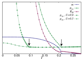
Figure 6: Solid lines: on-site magnetization ($m$), DC resistivity ($\rho_{xx}$) and Hall coefficient ($R_{H}$) for $t_{\sigma}=-1.2$ and $U=1.25$. The non-solid lines show $\rho_{xx}$ for $U=0.9$ and $0.5$. The arrows indicate the locations of the continuous transitions, at which $\rho_{xx}$ shows a rapid upturn. The vertical axis goes from zero to positive values in arbitrary units.

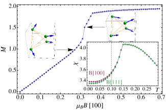
Figure 7: Main: magnetization per unit cell, $M$, as a function of an applied magnetic field along the [100] direction for the AIO insulator at $t_{\sigma}=-1.2$ and $U=2.1$. The evolution of the magnetic moments across an abrupt feature is shown. Inset: Susceptibility for fields along [100] and [111] versus $T$. The dashed line corresponds to the 2nd order transition.

V Magnetic field

We examine the effects of a magnetic field on some of the ground states of Fig. 2 via the addition of a Zeeman coupling to the Hubbard Hamiltonian. Since we ignore orbital coupling to the applied field, we focus on the non-metallic phases. We solve the self-consistent mean-field equations as above We have considered fields along the [100], [110] and [111] directions. In all cases, we find a rather continuous evolution to a fully polarized paramagnetic state, without any first order transition to a FM aligned with the field, in contrast with claims made in Ref. Wan et al., 2011. Instead, the net magnetization grows until it (asymptotically) reaches a fully polarized state, as shown in Fig. 7 for the case of the AF insulator at $t_{\sigma}=-1.2$ and $U=2.1$. The magnetization profiles generically present small features that correspond to sudden changes in the magnetic order (never to a FM, though), but lead to small changes in the actual magnetization. One such abrupt evolution is seen to occur around $\mu_{B}B\approx 0.32$ in Fig. 7. The magnetic susceptibility, $\chi$, as a function of temperature is shown in the inset of Fig. 7 for fields along [100] and [111]; with $\chi[110]=\chi[100]$. At temperatures above the magnetic melting transition, $T>T_{c}=0.148$, $\chi$ is isotropic and slowly varying. As $T$ is lowered, $\chi$ has a maximum at $T_{c}$, beyond which point it becomes slightly anisotropic. We find that in the ordered phase, $\chi[100]>\chi[111]$. All of these features are consistent with recent measurements of the zero-field cooled (ZFC) susceptibility of Eu-227Ishikawa et al. (2012).

VI Discussion

We have introduced a microsopically-motivated Hamiltonian for the pyrochlore iridates, which contains all symmetry-allowed terms up to NNN. Its ground states include semimetals and metals, topological insulators, topological Weyl semimetals, gapped AF states with the all-in/all-out and related orders. Our phase diagram, Fig. 2, and results for the transport and magnetic properties at finite $T$ and field suggest that our new model is apt to describe many salient features of the pyrochlore iridates family. In particular, in light of recent experimentsMatsuhira et al. (2007); Ishikawa et al. (2012); Tafti et al. (2012) that show the presence of a charge gap in Eu-227, we suggest that its ground state is an AIO gapped insulator, which under pressure can undergo a Lifshitz transition to a non-magnetic metal with small pockets, although TWS and metallic AF (with coexisting Weyl nodes and pockets) are possible. At sufficiently high temperatures, we find that the magnetic order melts continuously leading to a paramagnetic metal, consistent with experiments. For Y-227, which shows insulating behaviour at all temperatures ($d\rho/dT<0$), we suggest that the high temperature non-magnetic state (connected to the $U=0$ parent phase) is a semimetal. The TWS, which we find melts at relatively low temperatures, is probably not present in the ground states of Eu- and Y-227 because of the evidence for a finite gap but it might be accessible by hydrostatic pressureTafti et al. (2012); Sakata et al. (2011). Similarly, the ground state of Nd-227 was suggestedDisseler et al. (2012a) to be poised near a metal-insulator transition (on the insulating side), potentially in the vicinity of the TWS.

In closing, we mention recent experiments on Bi₂Ir₂O₇Qi et al. (2012); Baker et al. (2013) which shows some similar properties to the other rare-earth based pyrochlore iridates. It was found that the resistivity of Bi-227 remains metallic down to sub-Kelvin temperaturesQi et al. (2012), and recent $\mu$SR measurementsBaker et al. (2013) have found evidence for a continuous transition into a long-range magnetically ordered state at $\approx 2$ K. Moreover, the measurements suggest that the magnetic moments are very small. We observe that these features can be consistently fitted into our framework if we assume the ground state of Bi-227 is a metallic AF, see Fig. 2, which is obtained by “over-tilting” the TWS. Such a state carries the AIO order with small on-site moments. As a consequence, the continuous transition into a paramagnetic state occurs at a temperature much smaller than for the phases with a gapped AF ground state. An important caveat is that the Ir $d$-electrons will hybridize with the $s$- and $p$-orbitals of BiQi et al. (2012), a feature that we do not take into account. Nevertheless, since our effective model is quite general, it may not be unreasonable to expect that it will capture some features of Bi-227.

Appendix A Constructing the general Hamiltonian

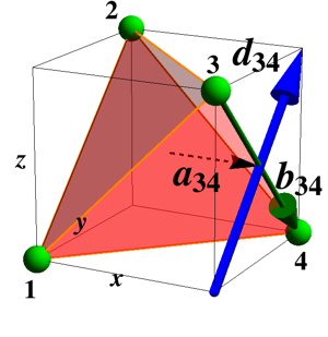
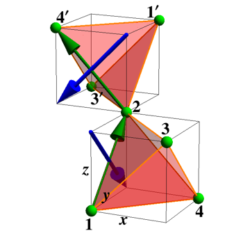
Figure 8: Definitions of vectors entering into the general Hamiltonian. The green (thin) arrows correspond to the ${\bm{b}}_{ij}$, whereas the blue (thick) ones to the ${\bm{d}}_{ij}$. b) shows the vectors involved in obtaining the NNN hopping amplitude between sites 1 and $4^{\prime}$, who share a common NN, site 2.

We provide details regarding the construction of the Hamiltonian used in the main text. We choose the basis vectors of the pyrochlore lattice to be Fig. 8 a): ${\bm{b}}_{1}=(0,0,0)\,,{\bm{b}}_{2}=(0,1,1)\,,{\bm{b}}_{3}=(1,0,1)\,,{\bm{b}}_{4}=(1,1,0)$. In these units the FCC unit cell has dimension $a=4$. As stated in the main text, the most general hopping Hamiltonian on the pyrochlore lattice takes the form:

$$H_{0}=\sum_{\begin{subarray}{c}\langle i,j\rangle\end{subarray}}c_{i}^{\dagger}(t_{1}+it_{2}{\bm{d}}_{ij}\cdot{\bm{\sigma}})c_{j}+\sum_{\begin{subarray}{c}\langle\langle i,j\rangle\rangle\end{subarray}}c_{i}^{\dagger}(t_{1}^{\prime}+i[t_{2}^{\prime}\bm{\mathcal{R}}_{ij}+t_{3}^{\prime}\bm{\mathcal{D}}_{ij}]\cdot{\bm{\sigma}})c_{j}\,,$$ (5)

where the NN Hamiltonian is built using the vectors:

$${\bm{d}}_{ij} =2{\bm{a}}_{ij}\times{\bm{b}}_{ij}\,,$$ (6)

$${\bm{a}}_{ij} =\frac{1}{2}({\bm{b}}_{i}+{\bm{b}}_{j})-{\bm{x}}_{c}\,,$$ (7)

$${\bm{b}}_{ij} ={\bm{b}}_{j}-{\bm{b}}_{i}\,,$$ (8)

where it is understood in these definitions that ${\bm{b}}_{i}$ selects the basis vector of the full lattice (Bravais + basis) index, $i$. ${\bm{a}}_{ij}$ points from the center of the tetrahedron, ${\bm{x}}_{c}=(1,1,1)/2$, to the middle of the $\langle i,j\rangle$ bond; it is always orthogonal to the faces of the cube built out of the tetrahedron’s vertices, see Fig. 8. ${\bm{b}}_{ij}$ is the NN bond vector pointing from site $i$ to site $j$. We have chosen the notation for the ${\bm{d}}_{ij}$ in analogy with the Dzyaloshinski-Morya (DM) vectors, ${\bm{D}}_{ij}$, of a spin model on the pyrochlore lattice because both sets of vectors are parallel or antiparallel on all bonds. The difference arises in the sign. There are only two symmetry-allowed configurations of DM vectorsElhajal et al. (2005); Witczak-Krempa and Kim (2012), differing by a global sign. The ${\bm{d}}_{ij}$’s are always found to differ by a sign on some bonds with either type of DM vectors.

The NNN Hamiltonian simply uses cross products of the ${\bm{b}}_{ij}$’s and ${\bm{d}}_{ij}$’s:

$$\bm{\mathcal{R}}_{ij} ={\bm{b}}_{ik}\times{\bm{b}}_{kj}\,,$$ (9)

$$\bm{\mathcal{D}}_{ij} ={\bm{d}}_{ik}\times{\bm{d}}_{kj}\,,$$ (10)

where $i$ and $j$ are NNNs and share the site $k$ as their (unique) common NN. $\bm{\mathcal{R}}_{ij},\bm{\mathcal{D}}_{ij}$ are obtained by going to the NNN via the common NN site and taking a cross product of the two bond or ${\bm{d}}$ vectors encountered, respectively. Fig. 8 b) illustrates the vectors necessary to construct the NNN amplitude between sites 1 and $4^{\prime}$. We note that $\bm{\mathcal{R}}_{ij}$ and $\bm{\mathcal{D}}_{ij}$ always point along the diagonals $(s_{1},s_{2},s_{3})$, where $s_{i}=\pm 1$. For instance, $\bm{\mathcal{R}}_{34}=(1,-1,1)$ and $\bm{\mathcal{D}}_{34}=(-1,1,1)$, as can be read off from Fig. 8; they are linearly independent as it should. For completeness, we provide the momentum-space form of the Hamiltonian, $H=\sum_{{\bm{q}}}c_{a}^{\dagger}({\bm{q}})(\mathcal{H}_{ab}^{\rm NN}({\bm{q}})+\mathcal{H}_{ab}^{\rm NNN}({\bm{q}}))c_{b}({\bm{q}})$, with

$$\mathcal{H}_{ab}^{\rm NN}({\bm{q}}) =2(t_{1}+t_{2}i{\bm{\sigma}}\cdot{\bm{d}}_{ab})\cos\left[{\bm{q}}\cdot{\bm{b}}_{ab}\right]\,,$$ (11)

$$\mathcal{H}_{ab}^{\rm NNN}({\bm{q}}) =2\sum_{c\neq a,b}\left\{t_{1}^{\prime}(1-\delta_{ab})+i{\bm{\sigma}}\cdot\left[t_{2}^{\prime}({\bm{b}}_{ac}\times{\bm{b}}_{cb})+t_{3}^{\prime}({\bm{d}}_{ac}\times{\bm{d}}_{cb})\right]\right\}\cos\left[{\bm{q}}\cdot(-{\bm{b}}_{ac}+{\bm{b}}_{cb})\right]\,,$$ (12)

where the indices $1\leq a,b,c\leq 4$ run over the basis sites. The sum over $c$ in the NNN Hamiltonian runs over the choice of common NN between NNNs on sublattices $a$ and $b$. There are two such sites: $c\in\{1,2,3,4\}\setminus\{a,b\}$.

Ref. Guo and Franz, 2009 discussed the $t_{1},t_{2}^{\prime}$ model, with a special focus on topological insulator phases. Ref. Kurita et al., 2011 identified the $t_{1},t_{2}$ model as the most general NN, time-reversal-invariant hopping Hamiltonian on the pyrochlore lattice, for a single (pseudo)spin-1/2 Hilbert space per site. (We note that these two works use ${\bm{d}}_{ij}$ to denote our ${\bm{b}}_{ij}$.)

A.1 Relation to microscopically motivated Hamiltonian

Two of us have previously proposed a model for the pyrochlore iridates, which was mainly analysed at the NN levelWitczak-Krempa and Kim (2012). It extends a previous onePesin and Balents (2010) (although we focus on 2 spin/orbital degrees of freedom per site instead of 6) to which we added hopping amplitudes arising from the direct overlaps of the d-orbitals of Ir. These Slater-Koster like models are more naturally constructed in a local basis because of the relative rotations between the oxygen octahedra within a unit cell, an illustration of this is found in Ref. Witczak-Krempa and Kim, 2012. It is however useful to consider the same Hamiltonians expressed in a global basis instead, to see the role of the different microscopic hoppings more clearly.

We have taken the microscopic, local-axis Hamiltonian given by Eq. (1) in Ref. Witczak-Krempa and Kim, 2012, supplemented by NNN direct hoppings, and have performed spinor rotations to obtain a Hamiltonian in a global basis for the pseudospin. This was compared with Eq. (5) to obtain the relation between $\{t_{1},t_{2},t_{1}^{\prime},t_{2}^{\prime},t_{3}^{\prime}\}$ and $\{t_{\rm oxy},t_{\sigma},t_{\pi},t_{\sigma}^{\prime},t_{\pi}^{\prime},t_{\delta}^{\prime}\}$, as given in the main text. Compared with the main body, we in addition include the NNN hopping arising from the $\delta$-overlap, $t_{\delta}^{\prime}$, leading to:

$$t_{1} =\frac{130t_{\rm oxy}}{243}+\frac{17t_{\sigma}}{324}-\frac{79t_{\pi}}{243};\quad\,\,t_{1}^{\prime}=\frac{233t_{\sigma}^{\prime}}{2916}-\frac{407t_{\pi}^{\prime}}{2187}-\frac{1843t_{\delta}^{\prime}}{8748}\,;$$

$$t_{2} =\frac{28t_{\rm oxy}}{243}+\frac{15t_{\sigma}}{243}-\frac{40t_{\pi}}{243};\,\;\;\;\;\quad t_{2}^{\prime}=\frac{t_{\sigma}^{\prime}}{1458}+\frac{220t_{\pi}^{\prime}}{2187}+\frac{277t_{\delta}^{\prime}}{4374}\,;$$

$$t_{3}^{\prime} =\frac{25t_{\sigma}^{\prime}}{1458}+\frac{460t_{\pi}^{\prime}}{2187}-\frac{275t_{\delta}^{\prime}}{4374}\,;$$ (13)

The NNN hopping $t_{\delta}^{\prime}$ was added in order to have a number of degrees of freedom matching that of the general Hamiltonian at the NNN level. One can also consider the NNN oxygen-mediated hopping, which will add an analogous term to the $t_{i}^{\prime}$. Fig. 9 shows the relation between $t_{\sigma}$ (in units of $t_{\rm oxy}$) and $t_{2}/t_{1}$, where we have set $t_{\pi}=-2t_{\sigma}/3$. The exact phase boundaries of the NN hopping Hamiltonian expressed using the Slater-Koster amplitudes can be obtained from the exact ones in the $t_{1}-t_{2}$ model, $t_{2}/t_{1}=-2,0$: $t_{\sigma}=-192/115,\;-84/125\approx-1.67,\;-0.67$, as can be verified in Fig. 9.

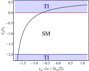
Figure 9: The curve shows the relation between $t_{\sigma}$ (in units of $t_{\rm oxy}$) and $t_{2}/t_{1}$, the latter coming from the general Hamiltonian Eq. (1).

References

- Kim et al. (2008) B. J. Kim, H. Jin, S. J. Moon, J.-Y. Kim, B.-G. Park, C. S. Leem, J. Yu, T. W. Noh, C. Kim, S.-J. Oh, J.-H. Park, V. Durairaj, G. Cao, and E. Rotenberg, Phys. Rev. Lett. 101, 076402 (2008).
- Kim et al. (2009) B. J. Kim, H. Ohsumi, T. Komesu, S. Sakai, T. Morita, H. Takagi, and T. Arima, Science 323, 1329 (2009).
- Pesin and Balents (2010) D. Pesin and L. Balents, Nat Phys 6, 376 (2010).
- Witczak-Krempa et al. (2010) W. Witczak-Krempa, T. P. Choy, and Y. B. Kim, Phys. Rev. B 82, 165122 (2010).
- Machida et al. (2009) Y. Machida, S. Nakatsuji, S. Onoda, T. Tayama, and T. Sakakibara, Nature 463, 210 (2009).
- Wan et al. (2011) X. Wan, A. M. Turner, A. Vishwanath, and S. Y. Savrasov, Phys. Rev. B 83, 205101 (2011).
- Witczak-Krempa and Kim (2012) W. Witczak-Krempa and Y. B. Kim, Phys. Rev. B 85, 045124 (2012).
- Go et al. (2012) A. Go, W. Witczak-Krempa, G. S. Jeon, K. Park, and Y. B. Kim, Phys. Rev. Lett. 109, 066401 (2012).
- Yanagishima and Maeno (2001) D. Yanagishima and Y. Maeno, Journal of the Physical Society of Japan 70, 2880 (2001).
- Taira et al. (2001) N. Taira, M. Wakeshima, and Y. Hinatsu, Journal of Physics: Condensed Matter 13, 5527+ (2001).
- Fukazawa and Maeno (2002) H. Fukazawa and Y. Maeno, Journal of the Physical Society of Japan 71, 2578 (2002).
- Matsuhira et al. (2007) K. Matsuhira, M. Wakeshima, R. Nakanishi, T. Yamada, A. Nakamura, W. Kawano, S. Takagi, and Y. Hinatsu, Journal of the Physical Society of Japan 76, 043706+ (2007).
- Matsuhira et al. (2011) K. Matsuhira, M. Wakeshima, Y. Hinatsu, and S. Takagi, Journal of the Physical Society of Japan 80, 094701 (2011).
- Hasegawa et al. (2010) T. Hasegawa, N. Ogita, K. Matsuhira, S. Takagi, M. Wakeshima, Y. Hinatsu, and M. Udagawa, Journal of Physics: Conference Series 200, 012054+ (2010).
- Zhao et al. (2011) S. Zhao, J. M. Mackie, D. E. MacLaughlin, O. O. Bernal, J. J. Ishikawa, Y. Ohta, and S. Nakatsuji, Phys. Rev. B 83, 180402 (2011).
- Ishikawa et al. (2012) J. J. Ishikawa, E. C. T. O’Farrell, and S. Nakatsuji, Phys. Rev. B 85, 245109 (2012).
- Tomiyasu et al. (2012) K. Tomiyasu, K. Matsuhira, K. Iwasa, M. Watahiki, S. Takagi, M. Wakeshima, Y. Hinatsu, M. Yokoyama, K. Ohoyama, and K. Yamada, Journal of the Physical Society of Japan 81, 034709+ (2012).
- Tafti et al. (2012) F. F. Tafti, J. J. Ishikawa, A. McCollam, S. Nakatsuji, and S. R. Julian, Phys. Rev. B 85, 205104 (2012).
- Sakata et al. (2011) M. Sakata, T. Kagayama, K. Shimizu, K. Matsuhira, S. Takagi, M. Wakeshima, and Y. Hinatsu, Phys. Rev. B 83, 041102 (2011).
- Shapiro et al. (2012) M. C. Shapiro, S. C. Riggs, M. B. Stone, C. R. de la Cruz, S. Chi, A. A. Podlesnyak, and I. R. Fisher, Phys. Rev. B 85, 214434 (2012).
- Disseler et al. (2012a) S. M. Disseler, C. Dhital, T. C. Hogan, A. Amato, S. R. Giblin, C. de la Cruz, A. Daoud-Aladine, S. D. Wilson, and M. J. Graf, Phys. Rev. B 85, 174441 (2012a).
- Disseler et al. (2012b) S. M. Disseler, C. Dhital, A. Amato, S. R. Giblin, C. de la Cruz, S. D. Wilson, and M. J. Graf, Phys. Rev. B 86, 014428 (2012b).
- Chen and Hermele (2012) G. Chen and M. Hermele, Phys. Rev. B 86, 235129 (2012).
- Yang and Kim (2010) B.-J. Yang and Y. B. Kim, Phys. Rev. B 82, 085111 (2010).
- Kargarian et al. (2011) M. Kargarian, J. Wen, and G. A. Fiete, Phys. Rev. B 83, 165112 (2011).
- Elhajal et al. (2005) M. Elhajal, B. Canals, R. Sunyer, and C. Lacroix, Phys. Rev. B 71, 094420 (2005).
- Moore and Balents (2007) J. E. Moore and L. Balents, Phys. Rev. B 75, 121306 (2007).
- Roy (2009) R. Roy, Phys. Rev. B 79, 195322 (2009).
- Fu et al. (2007) L. Fu, C. L. Kane, and E. J. Mele, Phys. Rev. Lett. 98, 106803 (2007).
- Guo and Franz (2009) H.-M. Guo and M. Franz, Phys. Rev. Lett. 103, 206805 (2009).
- Kurita et al. (2011) M. Kurita, Y. Yamaji, and M. Imada, Journal of the Physical Society of Japan 80, 044708+ (2011).
- Ong (1991) N. P. Ong, Phys. Rev. B 43, 193 (1991).
- Podolsky and Kim (2011) D. Podolsky and Y. B. Kim, Phys. Rev. B 83, 054401 (2011).
- Qi et al. (2012) T. F. Qi, O. B. Korneta, X. Wan, L. E. DeLong, P. Schlottmann, and G. Cao, Journal of Physics: Condensed Matter 24, 345601 (2012).
- Baker et al. (2013) P. J. Baker, J. S. Moeller, F. L. Pratt, W. Hayes, S. J. Blundell, T. Lancaster, T. F. Qi, and G. Cao, ArXiv e-prints (2013), arXiv:1302.6905 [cond-mat.str-el] .