Interpreting the conformal cousin of the Husain-Martinez-Nuñez spacetime

Abstract

A 2-parameter inhomogeneous cosmology in Brans-Dicke theory, obtained by conformally transforming the Husain-Martinez-Nuñez scalar field solution of the Einstein equations is studied and interpreted physically. According to the values of the parameters it describes a wormhole or a naked singularity. The reasons why there isn’t a one-to-one correspondence between conformal copies of this metric are discussed.

I Introduction

In their low-energy limit, most theories attempting to quantize gravity produce modifications of general relativity in the form of non-minimally coupled dilaton fields and/or higher derivative terms in the gravitational sector (this is the case, for example, of the bosonic string theory which reduces to an $\omega=-1$ Brans-Dicke theory bosonic ). Attempts to explain the present-day cosmological acceleration discovered using the luminosity distance-redshift relation of type Ia supernovae SN without introducing the ad hoc dark energy has led, among other scenarios, to infrared modifications of gravity CCT . This “$f(R)$” gravity is nothing but a Brans-Dicke theory with a special scalar field potential (see f(R)reviews for reviews).

Several alternative theories of gravity have been proposed and studied recently, as low-energy effective actions or as toy models for quantum or emergent gravity, or in the context of early or late universe cosmology (see CliftonPadillaetc for a recent review). In addition, varying “constants” of nature hypothesized by Dirac Dirac can be implemented naturally in scalar-tensor gravity, in which the gravitational coupling depends on the spacetime point BD ; ST .

When approaching a theory of gravity, it is important to understand its spherically symmetric solutions and, in particular, its black holes. Solutions of the field equations describing inhomogeneities in cosmological spaces have been studied with the specific purpose of modelling spatial variations of the gravitational coupling varyingG ; CMB . Spherically symmetric inhomogeneous solutions of Brans-Dicke gravity which describe a central condensation embedded in a Friedmann-Lemaître-Robertson-Walker (FLRW) background have been found, but not studied or interpreted, in Ref. CMB . Extra value is added to the study of spacetimes describing central objects in cosmological backgrounds by the fact that such metrics are not well understood even in the context of Einstein theory McVittie ; Klebanetal ; Roshina ; LakeAbdelqader ; AndresRoshina . Moreover, the old problem of the influence of the cosmic expansion on local dynamics (and vice-versa), which originally led to the study of such solutions McVittie , is not completely solved CarreraGiulini .

In this paper we analyze a Brans-Dicke solution found by Clifton, Mota, and Barrow CMB and describing an inhomogeneity embedded in a FLRW universe. This solution is generated using a conformal transformation and the Husain-Martinez-Nuñez scalar field solution of general relativity HMN as a seed. The conformal copy is not a perfect mirror image of the original solution, however, because it is found (in Sec. II) that it describes a spacetime with properties quite different from the original one. This fact should not lead to superficial statements on the physical inequivalence between conformal frames because the usual conformal mapping between Brans-Dicke’s and Einstein’s theories (and their solutions) prescribes also a scaling of units in the Einstein frame Dicke which went lost in Ref. CMB , where the authors intended only to generate a new spherical and inhomogeneous solution of the Brans-Dicke field equations. Sec. IV contains a discussion on this subject.

II Understanding the Clifton-Mota-Barrow spacetime

Clifton, Mota, and Barrow CMB conformally mapped the spherically symmetric and dynamical Husain-Martinez-Nuñez HMN scalar field solution of general relativity to obtain the 2-parameter class of Brans-Dicke spacetimes

$$ds^{2}=-A^{\alpha\left(1-\frac{1}{\sqrt{3}\,\beta}\right)}(r)\,dt^{2}+A^{-\alpha\left(1+\frac{1}{\sqrt{3}\,\beta}\right)}(r)\,t^{\frac{2\left(\beta-\sqrt{3}\right)}{3\beta-\sqrt{3}}}\left[dr^{2}+r^{2}A(r)d\Omega_{(2)}^{2}\right]\,,$$ (1)

$$\phi(t,r)=A^{\frac{\pm 1}{2\beta}}(r)\,t^{\frac{2}{\sqrt{3}\,\beta-1}}\,,$$ (2)

where $d\Omega_{(2)}^{2}=d\theta^{2}+\sin^{2}\theta\,d\varphi^{2}$ is the metric on the unit 2-sphere,

$$A(r) = 1-\frac{2C}{r}\,,$$ (3)

$$\alpha = \pm\,\frac{\sqrt{3}}{2}\,,$$ (4)

$$\beta = \sqrt{2\omega+3}\,,$$ (5)

$C$ is a parameter related to the mass of the central inhomogeneity, and $\omega$ is the Brans-Dicke coupling parameter which is required to be larger than $-3/2$. We adopt the notations of Ref. Wald . There are spacetime singularities at $r=2C$ and at $t=0$, therefore, the relevant coordinate range is $2C<r<+\infty$ and $t>0$ CMB . The scale factor of the spatially flat FLRW background universe is

$$a(t)=t^{\frac{\beta-\sqrt{3}}{3\beta-\sqrt{3}}}\equiv t^{\gamma}\,.$$ (6)

The line element (1) can be rewritten as

$$ds^{2}=-A^{\sigma}(r)\,dt^{2}+A^{\Theta}(r)\,a^{2}(t)dr^{2}+R^{2}(t,r)d\Omega_{(2)}^{2}\,,$$ (7)

where

$$\sigma = \alpha\left(1-\frac{1}{\sqrt{3}\,\beta}\right)\,,$$ (8)

$$\Theta = -\alpha\left(1+\frac{1}{\sqrt{3}\,\beta}\right)\,,$$ (9)

and

$$R(t,r)=A^{\frac{\Theta+1}{2}}(r)\,a(t)r$$ (10)

is the areal radius.

Let us examine the behaviour of the area $4\pi R^{2}$ of 2-spheres of symmetry by studying how the areal radius behaves as a function of $r$. We have

$$\frac{\partial R}{\partial r} = a(t)A^{\frac{\Theta-1}{2}}(r)\left[1-\frac{2C}{r}\,\frac{\left(1-\Theta\right)}{2}\right]$$ (11)

$$\equiv a(t)A^{\frac{\Theta-1}{2}}(r)\left(1-\frac{r_{0}}{r}\right)\,,$$

where

$$r_{0}=(1-\Theta)C$$ (12)

or, in terms of the proper (areal) radius,

$$R_{0}(t)=\left(\frac{\Theta+1}{\Theta-1}\right)^{\frac{\Theta+1}{2}}(1-\Theta)a(t)\,C\,.$$ (13)

The critical value $r_{0}$ exists in the relevant spacetime region $r_{0}>2C$ if $\Theta<-1$. In this case the areal radius can be written as

$$R(r)=\frac{ra(t)}{\left(1-\frac{2C}{r}\right)^{|\frac{\Theta+1}{2}|}}$$ (14)

and $R(r)\rightarrow+\infty$ as $r\rightarrow 2C^{+}$: the area of 2-spheres of symmetry diverges as $r\rightarrow 2C^{+}$. Due to eq. (11), for $\Theta<-1$ we have $\frac{1-\Theta}{2}>1$ and $\partial R/\partial r>0$ for $r$ larger than

$$r_{0}=2C\left(\frac{1-\Theta}{2}\right)>2C\,,$$ (15)

$\partial R/\partial r=0$ at $r=r_{0}$, and $\partial R/\partial r<0$ for $r<r_{0}$. The function $R(r)$ has a minimum at $r_{0}$ (fig. 1).

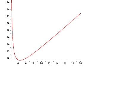
Figure 1: the areal radius $R$ (vertical axis) as a function of $r$ (horizontal axis) for the parameter values $\alpha=\sqrt{3}/2,\Theta=-3/2$, and $C=1$ (in units of $C$) at a time $t_{*}$ at which $a(t_{*})=1$.

The area of 2-spheres of symmetry decreases between $2C$ and $r_{0}$, where it is minimum, then it increases again. There is a wormhole throat joining two spacetime regions (cf. Ref. Hayward for a detailed wormhole theory). Note that, since

$$\Theta=\mp\frac{\sqrt{3}}{2}\left(1+\frac{1}{\sqrt{3}\sqrt{2\omega+3}}\right)$$ (16)

for $\alpha=\pm\sqrt{3}/2$, the condition $\Theta<-1$ requires $\alpha=+\sqrt{3}/2$. This value of $\alpha$, however, is a necessary but not a sufficient condition for the apparent horizon to exist. The sufficient condition $\Theta<-1$ imposes the constraint on the Brans-Dicke parameter

$$\omega<\frac{1}{2}\left[\frac{1}{\left(2-\sqrt{3}\right)^{2}}-3\right]\equiv\omega_{0}\,,$$ (17)

which can be satisfied in the allowed parameter region $\omega>-3/2$. Therefore, for $-3/2<\omega<\omega_{0}$ there is an apparent horizon at $r_{0}>2C$ and the solution can be taken to represent a Brans-Dicke wormhole. Here by “wormhole” we simply refer to a spacetime containing a smooth wormhole throat connecting two spacetime regions. Other definitions of wormhole (for example, a generalization to the dynamical case of the definition of Ref. Bronnikov ) are more stringent and would not allow this spacetime to be called a wormhole.

The region $2C<r<r_{0}$ is not a FLRW region and the scalar field (2) is finite and non-zero at $r_{0}$:

$$\phi\left(t,r_{0}\right)=t^{\frac{2}{\sqrt[]{3}\beta-1}}\left(\frac{\Theta+1}{\Theta-1}\right)^{\frac{\pm 1}{2\beta}}\,.$$ (18)

The proper radius (13) of the wormhole throat is exactly comoving with the cosmic substratum and disappears if the central inhomogeneity is removed, which is formally described by the limit $C\rightarrow 0$.

Let us now investigate the presence of apparent horizons in the metric (1). Using eq. (10) and substituting the relation between differentials

$$dr=\frac{dR-A^{\frac{\Theta+1}{2}}(r)\,\dot{a}(t)rdt}{A^{\frac{\Theta-1}{2}}a(t)\,\frac{C(\Theta+1)}{r}+A^{\frac{\Theta+1}{2}}(r)\,a(t)}\,,$$ (19)

into the line element (7), one obtains

$$ds^{2} = -A^{\sigma}dt^{2}+\left[\frac{dR^{2}-2A^{\frac{\Theta+1}{2}}r\dot{a}\,dtdR+A^{\frac{\Theta+1}{2}}r^{2}\dot{a}^{2}dt^{2}}{D_{1}(r)}\right]$$ (20)

$$+R^{2}d\Omega_{(2)}^{2}\,,$$

where

$$D_{1}(r)=A(r)\left[1+\frac{C(\Theta+1)}{rA(r)}\right]^{2}\,.$$ (21)

Collecting similar terms yields

$$ds^{2} = -\frac{\left(D_{1}A^{\sigma}-H^{2}R^{2}\right)}{D_{1}}\,dt^{2}-\frac{2HR}{D_{1}}\,dtdR+\frac{dR^{2}}{D_{1}}$$ (22)

$$+R^{2}d\Omega_{(2)}^{2}\,,$$

where $H\equiv\dot{a}/a$ is the Hubble parameter of the background universe. The inverse of the metric $g_{\mu\nu}$ of eq. (22) is

$$\left(g^{\mu\nu}\right)=\left(\begin{array}[]{cccc}-\frac{1}{A^{\sigma}}&-\frac{HR}{A^{\sigma}}&0&0\\ &&&\\ -\frac{HR}{A^{\sigma}}&\frac{\left(D_{1}A^{\sigma}-H^{2}R^{2}\right)}{A^{\sigma}}&0&0\\ &&&\\ 0&0&\frac{1}{R^{2}}&0\\ &&&\\ 0&0&0&\frac{1}{R^{2}\sin^{2}\theta}\end{array}\right).$$ (23)

In the presence of spherical symmetry the apparent horizons are located by the roots of the equation $\nabla^{c}R\nabla_{c}R=0$ (e.g., NielsenVisser ) or $g^{RR}=0$, which here yields

$$D_{1}(r)A(r)=H^{2}(t)R^{2}(t,r)\,.$$ (24)

The left hand side of this equation depends only on $r$ while the right hand side depends on both $r$ and $t$. This equation can only be satisfied when the right hand side is time-independent and the only possibility for this to occur is when $H=\gamma/t=0$, corresponding to $\gamma=0$, $\beta=\sqrt{3}$, and $\omega=0$. This value of the Brans-Dicke parameter gives a static solution describing a spherical inhomogeneity in a Minkowski background, which is discussed in the next section. With this exception, eq. (24) has no solutions and there are no apparent horizons in the spacetime (1). In particular, for $\Theta<-1$ the wormhole throat is not an apparent horizon.

Let us discuss now the case $\omega\geq\omega_{0}$ and the case $\alpha=-\sqrt{3}/2$. In these situations there is no wormhole throat and no apparent horizon in the $r>2C$ region and the Clifton-Mota-Barrow spacetime contains a naked singularity.

For $\alpha=-\sqrt{3}/2$ it is $\Theta=\frac{\sqrt{3}}{2}\left(1+\frac{1}{\sqrt{3}\,\beta}\right)>0$ and

$$R(r)=\left(1-\frac{2C}{r}\right)^{\frac{|\Theta+1|}{2}}a(t)r$$ (25)

goes to zero as $r\rightarrow 2C^{+}$. Since $r_{0}<2C$, the areal radius $R(r)$ is always an increasing function of $r$ in the relevant range $2C<r<+\infty$. This spacetime contains a naked singularity at $R=0$.

III The special case $\omega=0$

The value $\omega=0$ of the Brans-Dicke coupling, corresponding to $\beta=\sqrt{3}$ and $\gamma=0$, produces the static metric

$$ds^{2}=-A^{\frac{2\alpha}{3}}(r)dt^{2}+\frac{dr^{2}}{A^{\frac{4\alpha}{3}}(r)}+\frac{r^{2}}{A^{\frac{4\alpha}{3}-1}(r)}\,d\Omega_{(2)}^{2}$$ (26)

and the scalar field

$$\phi(t,r)=A^{\frac{\pm 1}{2\sqrt{3}}}(r)t\,,$$ (27)

which is time-dependent even though the metric is static.

The metric (26) is easily identified as a member of the Campanelli-Lousto class CampanelliLousto . The general Campanelli-Lousto solution has the form

$$ds^{2} = -A^{b+1}(r)dt^{2}+\frac{dr^{2}}{A^{a+1}(r)}+\frac{r^{2}d\Omega_{(2)}^{2}}{A^{a}(r)}\,,$$ (28)

$$\phi(r) = \phi_{0}A^{\frac{a-b}{2}}(r)\,,$$ (29)

and $\phi_{0},a$, and $b$ are constants with $\phi_{0}>0$. The Brans-Dicke parameter is given by CampanelliLousto

$$\omega(a,b)=-2\,\frac{\left(a^{2}+b^{2}-ab+a+b\right)}{\left(a-b\right)^{2}}\,.$$ (30)

In the case of the metric (26) setting

$$\left(a,b\right)=\left(\frac{4\alpha}{3}-1,\frac{2\alpha}{3}-1\right)$$ (31)

reproduces the Campanelli-Lousto metric (28). Then, the expression (30) gives $\omega\left(\frac{4\alpha}{3}-1,\frac{2\alpha}{3}-1\right)=0$ for $\alpha=\pm\sqrt{3}/2$. However, the scalar field (27) differs from the Campanelli-Lousto scalar (29) by the linear dependence on the time $t$. Thus, the static limit of the Clifton-Mota-Barrow solution provides a (rather trivial) generalization of a Campanelli-Lousto solution.

The nature of the Campanelli-Lousto spacetime depends on the sign of the parameter $a$ VZF which, in our case, corresponds to the choice $\alpha=\sqrt{3}/2$ or $-\sqrt{3}/2$. For $a\geq 0$ (corresponding to $\alpha=+\sqrt{3}/2,a\simeq 0.1547$, and $\Theta=-\frac{4\alpha}{3}\simeq-1.1547<-1$) the Campanelli-Lousto spacetime contains a wormhole throat coinciding with an apparent horizon and located at $r_{0}=2C\left(\frac{1-\Theta}{2}\right)>2C$ VZF . This is consistent with eq. (24) with $H=0$ since, in this case, the equation $g^{RR}=0$ locating the apparent horizons reduces to $D_{1}(r)=0$ which yields again the root $r_{0}=C(1-\Theta)$ lying in the physical region $r>2C$. This is the only case in which the Clifton-Mota-Barrow solution under study contains an apparent horizon.

For $a<0$ (which is reproduced by the choice $\alpha=-\sqrt{3}/2$ and gives $a\simeq-2.1547$ and $\Theta\simeq 1.1547>0$) there are no apparent horizons and the spacetime contains a naked singularity VZF . This is consistent with the fact that eq. (24) with $H=0$ can only be satisfied if $D_{1}(r)=0$ and in this case there are no acceptable solutions because $r_{0}<2C$.

IV Discussion and conclusions

According to the parameter values, the Clifton-Mota-Barrow spacetime (1) contains a wormhole or a naked singularity (black holes, wormholes, and naked singularities could in principle be distinguished observationally through gravitational lensing lensing ). In the last situation, this solution of the Brans-Dicke field equations cannot be obtained as the development of regular Cauchy data.

One question which arises is the following: the Husain-Martinez-Nuñez and the Clifton-Mota-Barrow spacetimes are conformally related. As explained long ago by Dicke Dicke , the Jordan and the Einstein conformal frames should be different representations of the same physics (provided that the conformal transformation does not break down)—this issue has been the subject of a lively debate but has been shown to be largely a pseudo-problem (see Flanagan ; FaraoniNadeau ; DeruelleSasaki and the references therein). Then, why does the same solution look so different in the two different conformal frames for the parameter values for which a Jordan frame wormhole or naked singularity (1) corresponds to the Einstein frame black hole of HMN ? The answer is that, by following the more ordinary route and conformally transforming the Clifton-Mota-Barrow metric and scalar field (1) to the Einstein frame would produce the Husain-Martinez-Nuñez metric with scaling units of length, time and mass. What is physically relevant is the ratio of a physical quantity to its unit, and the units change with the spacetime position. Specifically, the units of length and time scale as the conformal factor $\Omega$, while the unit of mass scales as $\Omega^{-1}$ and derived units scale accordingly Dicke . In the Einstein frame, matter is coupled non-minimally to the metric while in the Jordan frame matter is minimally coupled. The scaling of units in the Einstein frame goes hand in hand with the non-minimal coupling of matter to the metric. In vacuo (which is the situation contemplated here), the non-minimal coupling of matter is forgotten, but the scaling of units should be remembered.

Another issue is that, contrary to event horizons (which are null surfaces and are conformally invariant), apparent horizons (which can be spacelike or even timelike) are not conformally invariant and change location under a conformal transformation AlexValerio . In order to characterize the properties of a dynamical black hole when conformal transformations are involved, one should not consider the apparent horizons of a metric but a new surface characterized by an entropy 2-form, as explained in detail in AlexValerio and AlexFirouzjaee . The new prescription of AlexValerio takes into account the scaling of units in the Einstein frame.

Therefore, a metric obtained from the conformal transformation to the Einstein frame of a seed Jordan frame metric with the extra information that units are scaling is quite different from the same formal metric with fixed units, which explains why conformally related spacetimes can look very different. Clifton, Mota, and Barrow took the Husain-Martinez-Nuñez solution of general relativity with fixed units and used it as a seed to generate a new class of solutions of Brans-Dicke gravity—they did not worry about generating a physically equivalent solution, which would have required to take into account scaling units. This procedure is certainly legitimate and achieves the goal, but it generates physically inequivalent spacetimes when the requirement of scaling units is dropped. Indeed, there are comments in the literature about the fact that conformally related solutions of Brans-Dicke theory and of the Einstein equations do not share the same properties coldBHs . A similar situation occurs with the Campanelli-Lousto solutions of Brans-Dicke theory CampanelliLousto , which relate to Fisher-Janis-Newman-Winicour solutions of the Einstein equations in the Einstein frame VZF , and with the veiled black holes of DeruelleSasaki ; AlexValerio ; AlexFirouzjaee (see VZF for a detailed discussion). To conclude, the physical nature of the Clifton-Mota-Barrow class of solutions is now clear and they do not cause problems for the interpretation of conformal frames.

- (1) C.G. Callan, D. Friedan, E.J. Martinez, and M.J. Perry, Nucl. Phys. B 262 (1985) 593; E.S. Fradkin and A.A. Tseytlin, Nucl. Phys. B 261 (1985) 1.
- (2) A.G. Riess et al., Astron. J. 116 (1998) 1009; Astron. J. 118 (1999) 2668; Astrophys. J. 560 (2001) 49; Astrophys. J. 607 (2004) 665; S. Perlmutter et al., Nature 391 (1998) 51; Astrophys. J. 517 (1999) 565; J.L. Tonry et al., Astrophys. J. 594 (2003) 1; R. Knop et al., Astrophys. J. 598 (2003) 102; B. Barris et al., Astrophys. J. 602 (2004) 571.
- (3) S. Capozziello, S. Carloni and A. Troisi, arXiv:astro-ph/0303041; S.M. Carroll, V. Duvvuri, M. Trodden and M.S. Turner, Phys. Rev. D 70 (2004) 043528; D.N. Vollick, Phys. Rev. D 68 (2003) 063510.
- (4) T.P. Sotiriou and V. Faraoni, Rev. Mod. Phys. 82 (2010) 451; A. De Felice and S. Tsujikawa, Living Rev. Rel. 13 (2010) 3; S. Capozziello and V. Faraoni, Beyond Einstein Gravity (Springer, New York, 2010).
- (5) T. Clifton, P.G. Ferreira, A. Padilla, and C. Skordis, Phys. Reps. 513 (2012) 1.
- (6) P.A.M. Dirac, Nature 139 (1937) 1001; Proc. Roy. Soc. Lon. A 165 (1938) 199; 333 (1973) 403.
- (7) C.H. Brans and R.H. Dicke, Phys. Rev. 124 (1961) 925.
- (8) P.G. Bergmann, Int. J. Theor. Phys. 1 (1968) 25; R.V. Wagoner, Phys. Rev. D 1 (1970) 3209; K. Nordvedt, Astrophys. J. 161 (1970) 1059.
- (9) J.D. Barrow and C. O’Toole, Mon. Not. Roy. Astron. Soc. 322 (2001) 585; N. Sakai and J.D. Barrow, Class. Quantum Grav. 18 (2001) 4717.
- (10) T. Clifton, D.F. Mota, and J.D. Barrow, Mon. Not. Roy. Astron. Soc. 358 (2005) 601.
- (11) G.C. McVittie, Mon. Not. Roy. Astron. Soc. 93 (1933) 325.
- (12) N. Kaloper, M. Kleban and D. Martin, Phys. Rev. D 81 (2010) 104044.
- (13) R. Nandra, A.N. Lasenby, and M.P. Hobson, Mon. Not. Roy. Astron. Soc. 422 (2012) 2931; Mon. Not. Roy. Astron. Soc. 422 (2012) 2945.
- (14) K. Lake and M. Abdelqader, Phys. Rev. D 84 (2011) 044045.
- (15) V. Faraoni, A.F. Zambrano Moreno, and R. Nandra, Phys. Rev. D 85 (2012) 083526.
- (16) M. Carrera and D. Giulini, Rev. Mod. Phys. 82 (2010) 169.
- (17) V. Husain, E.A. Martinez, and D. Nuñez, Phys. Rev. D 50 (1994) 3783.
- (18) R.H. Dicke, Phys. Rev. 125 (1962) 2163.
- (19) R.M. Wald, General Relativity (Chicago University Press, Chicago, 1984).
- (20) A.B. Nielsen and M. Visser, Class. Quantum Grav. 23 (2006) 4637; G. Abreu and M. Visser, Phys. Rev. D 82 (2010) 044027.
- (21) S.A. Hayward, Phys. Rev. D 79 (2009) 124001.
- (22) K.A. Bronnikov, M.V. Skortsova, and A.A. Starobinsky, Gravit. Cosmol. 16 (2010) 216.
- (23) V. Faraoni, V. Vitagliano, T.P. Sotiriou, and S. Liberati, preprint arXiv:1205.3945.
- (24) J.G. Cramer, R.L. Forward, M.S. Morris, M. Visser, G. Benford, and G.A. Landis, Phys. Rev. D 51 (1995) 3117; K.S. Virbhadra, D. Narashima, and S.M. Chitre, Astron. Astrophys. 337 (1998) 1; E. Eiroa, G.E. Romero, and D.F. Torres, Mod. Phys. Lett. A 16 (2001) 973; K.S. Virbhadra and G.F.R. Ellis, Phys. Rev. D 65 (2002) 103004; J.M. Tejeiro and E.A. Larranaga, arXiv:gr-qc/0505054; K.K. Nandi and Y.-Z. Zhang, Phys. Rev. D 74 (2006) 024020; T.K. Dey and S. Sen, Mod. Phys. Lett. A 23 (2008) 953; K.S. Virbhadra and C.R. Keeton, Phys. Rev. D 77 (2008) 124014. S. Sahu, M. Patil, D. Narasimha, and P.S. Joshi, Phys. Rev. D 86 (2012) 063010.
- (25) E.E. Flanagan, Class. Quantum Grav. 21 (2004) 3817.
- (26) V. Faraoni and S. Nadeau, Phys. Rev. D 75 (2007) 023501.
- (27) N. Deruelle and M. Sasaki, arXiv:1007.3563.
- (28) V. Faraoni and A.B. Nielsen, Class. Quantum Grav. 28 (2011) 175008.
- (29) A.B. Nielsen and J.T. Firouzajee, arXiv:1207.0064.
- (30) K.A. Bronnikov, M.S. Chernakova, J.C. Fabris, N. Pinto-Neto, and M.E. Rodrigues, Int. J. Mod. Phys. D 17 (2008) 25; P.E. Bloomfield, Phys. Rev. D 59 (1999) 088501; K.K. Nandi, B. Bhattacharjee, S.M.K. Alam, and J. Evans, Phys. Rev. D 57 (1998) 823.
- (31) M. Campanelli and C. Lousto, Int. J. Mod. Phys. D 2 (1993) 451; C. Lousto and M. Campanelli, in The Origin of Structure in the Universe, Proceedings, Pont d’Oye, Belgium 1992, E. Gunzig and P. Nardone eds. (Kluwer Academic, Dordrecht, 1993), p. 123.
- (32) L. Vanzo, S. Zerbini, and V. Faraoni, arXiv:1208.2513.