On the Use of Latency Graphs for
the Construction of Tor Circuits

Abstract

The use of anonymity-based infrastructures and anonymisers is a plausible solution to mitigate privacy problems on the Internet. Tor (short for The onion router) is a popular low-latency anonymity system that can be installed as an end-user application on a wide range of operating systems to redirect the traffic through a series of anonymising proxy circuits. The construction of these circuits determines both the latency and the anonymity degree of the Tor anonymity system. While some circuit construction strategies lead to delays which are tolerated for activities like Web browsing, they can make the system vulnerable to linking attacks. We evaluate in this paper three classical strategies for the construction of Tor circuits, with respect to their de-anonymisation risk and latency performance. We then develop a new circuit selection algorithm that considerably reduces the success probability of linking attacks while keeping a good degree of performance. We finally conduct experiments on a real-world Tor deployment over PlanetLab. Our experimental results confirm the validity of our strategy and its performance increase for Web browsing.

Keywords: Anonymity, Privacy, Entropy, Graphs, Algorithmics.

1 Introduction

Several anonymity designs have been proposed in the literature with the objective of achieving anonymity on different network technologies. From simple pseudonyms [1] to complex unstructured protocols [2], anonymity solutions can offer either strong anonymity with high latency (useful for high latency services, such as email and usenet messages) or weak anonymity with low-latency (useful, for instance, for Web browsing). The most widely-used low-latency solution for traditional Internet communications is based on anonymous mixes and onion routing [3]. It is distributed as a free software implementation known as Tor (The onion router [4]). It can be installed as an end-user application on a wide range of operating systems to redirect the traffic of low-latency services with a very acceptable overhead. Tor’s objective is the protection of privacy of a sender as well as the contents of its messages. To do so, it transforms cryptographically those messages and mixes them via a circuit of routers. The circuit routes the message in an unpredictable way. The content of each message is encrypted for every router in the circuit, with the objective of achieving anonymous communication even if a set of routers are compromised by an adversary. Upon reception, a router decrypts the message using its private key to obtain the following hop and cryptographic material on the path. This path is initially defined at the beginning of the process. Only the entity that creates the circuit knows the complete path to deliver a given message. The last router of the path, the exit node, decrypts the last layer and delivers an unencrypted version of the message to its target.

Tor allows the construction of anonymous channels with latency enough to route traffic for services like the Web [5]. However, it might still impact its performance depending on the specific strategy used for the establishment of the channel. In this paper, we address the influence of circuit construction strategies on the anonymity degree of Tor. We first provide a formal definition of the selection of Tor nodes process, of the adversary model targeting the communication anonymity of Tor users, and an analytical expression to compute the anonymity degree of the Tor infrastructure based on the circuit construction criteria. Based on these definitions, we evaluate three classical strategies, with respect to their de-anonymisation risk, and regarding their performance for anonymising Internet traffic. We then present the construction of a new circuit selection algorithm that aims at reducing the success probability of linking attacks while providing enough performance for low-latency services. A series of experiments, conducted on a real-world Tor deployment over PlanetLab [6] confirm the validity of the new strategy, and show its superiority over the classical ones.

Paper organisation — Section 2 presents the rationale of our work. Section 3 evaluates the anonymity degree of three traditional strategies for the construction of Tor circuits. Section 4 presents our new strategy. Section 5 evaluates the anonymity degree of our solution. Section 6 experimentally evaluates the latency performance of each strategy using PlanetLab. Section 7 surveys related work. Section 8 concludes the paper.

2 Rationale

In this section, we introduce the notation, models, and core definitions that are necessary to understand the rationale of our work.

2.1 Tor circuit

Formally, we can describe a connection using the Tor network as follows. First, we define a client node $s$ called a client or onion proxy, and a destination server node $d$ which we want to interconnect to exchange data in an anonymous manner. Let $N$ be the set of nodes deployed in the Tor network, and $n=|N|$ the cardinality of the set. Let node $e\in N$ denote a specified node, called the entrance node, and $x\in N$ the exit node. Then, a Tor circuit is a sequence of nodes $C=\langle s,e,r_{1},r_{2},...,r_{l},x\rangle$, where $r_{i}\in N$ is any intermediary node. The nodes $e$, $x$, and $r_{i}$, $i\in\{1,...,l\}$, are also known as onion routers. We define the path of a circuit as the set of links (i.e., network connections) $P=\{a_{1},...,a_{l+2}\}$ associated to the Tor circuit, where $a_{1}=(s,e)$, $a_{2}=(e,r_{1})$, $a_{3}=(r_{1},r_{2})$, … , $a_{l+1}=(r_{l-1},r_{l})$, $a_{l+2}=(r_{l},x)$. The value $|P|=l+2$ is called the length of the circuit. A connection using the Tor network is composed by the client and destination nodes interconnected through a Tor circuit as follows:

$\underbrace{s\xrightarrow{a_{1}}e\xrightarrow{a_{2}}r_{1}\xrightarrow{a_{3}}r_{2}\xrightarrow{a_{4}}...\xrightarrow{a_{l}}r_{l-1}\xrightarrow{a_{l+1}}r_{l}\xrightarrow{a_{l+2}}x}_{\text{Tor network}}\rightarrow d$

2.2 Adversary model

The adversary assumed in our work relies on the threat model proposed by Syverson et al. in [7]. Such a pragmatic model considers that, regardless of the number of onion routers in a circuit, an adversary controlling the entrance and exit nodes would have enough information in order to compromise the communication anonymity of a Tor client. Indeed, when both nodes collude, and given that the entry node knows the source of the circuit, and the exit node knows the destination, they can use traffic analysis to link communication over the same circuit [8].

Assuming the model proposed in [7], then an adversary who controls $c>1$ nodes over the $n$ nodes in the Tor network can control an entry node with probability $(\frac{c}{n})$, and an exit node with probability $(\frac{c}{n})$. This way, the adversary may de-anonymise the traffic flowing on a controlled circuit (i.e., a circuit whose entry and exit nodes are controlled by the adversary) with probability $(\frac{c}{n})^{2}$ if the length of the circuit is greater than two; or $\frac{c(c-1)}{n^{2}}$ if the length of the circuit is equal to two (cf. [7] and citations thereof). Adversaries can determine when the nodes under their control are either entry or exit nodes for the same circuit stream by using attacks such timing-based attacks [9], fingerprinting [10], and several other existing attacks.

Let us observe that the aforementioned probability of success assumes that the probability of a node from being selected on a Tor circuit is randomly uniform, that is, the boundaries provided in [7] only apply to the standard (random) selection of nodes, hereinafter denoted as random selection of nodes strategy. Given that the goal of our paper is to evaluate alternative selection strategies, we shall adapt the model. Therefore, let $p_{1}$, $p_{2}$, $p_{3}$, $\ldots$, $p_{c}$ be the corresponding selection probabilities assigned by the circuit construction algorithm to each node controlled by the adversary, then the probability of success corresponds to the following expression:

$$(p_{1}+p_{2}+p_{3}+\ldots+p_{c})\cdot(p_{1}+p_{2}+p_{3}+\ldots+p_{c})$$

that can be simplified as:

$$\Big{(}\sum_{i=1}^{c}p_{i}\Big{)}^{2}$$

Following is the analysis.

Theorem 2.1

Let $c$ be the number of nodes controlled by the adversary. Let the Tor client use a selection criteria which, for a certain circuit, every node selection is independent. Let $p_{1}$, $p_{2}$, $p_{3}$, $\ldots$, $p_{c}$ be the corresponding selection probabilities assigned by the circuit construction algorithm to each node controlled by the adversary. Then, the success of the adversary to compromise the security of the circuit is bounded by the following probability:

$$\Big{(}\sum_{i=1}^{c}p_{i}\Big{)}^{2}$$

Proof

The proof is direct by using the sum and product rules of probability theory, and taking into account that the selection of every node is an independent event. First, the probability of selecting the entrance or exit node in the set of nodes controlled by the adversary is (sum rule):

$$\sum_{i=1}^{c}p_{i}$$

Then, the probability of selecting, at the same time, a controlled entrance and exit node in a circuit is (product rule):

$$\Big{(}\sum_{i=1}^{c}p_{i}\Big{)}\Big{(}\sum_{i=1}^{c}p_{i}\Big{)}=\Big{(}\sum_{i=1}^{c}p_{i}\Big{)}^{2}$$

Corollary 1

The Syverson et al. success probability boundary in [7], i.e., $(\frac{c}{n})^{2}$, is equivalent to the boundary defined in Theorem 2.1 when the circuit selection criteria is a random selection of nodes.

Proof

Let $N$ be the set of nodes deployed in a Tor network with $n=|N|$, and let $A\subseteq N$ be the subset of nodes controlled by an adversary with $c=|A|$. The probability of a node $n_{i}\in N$ to be selected is $p_{i}=\frac{1}{n}$. Then, by applying it to the boundary defined in Theorem 2.1, we obtain:

$$\Big{(}\sum_{i=1}^{c}p_{i}\Big{)}^{2}=(c\cdot p_{i})^{2}=\Big{(}c\frac{1}{n}\Big{)}^{2}=\Big{(}\frac{c}{n}\Big{)}^{2}$$

2.3 Anonymity degree

Most work in the related literature has used the (Shannon) entropy concept to measure the anonymity degree of anonymisers like Tor (cf. [11, 12] and citations thereof). We recall that the entropy is a measure of the uncertainty associated with a random variable, that can efficiently be adapted to address new networking research problems [13, 14, 15]. In this paper, the entropy concept is used to determine how predictable is the selection of the nodes in accordance to a given strategy or, in other words, how easy is to violate the anonymity in relation to the adversary model defined in Section 2.2. Formally, given a probability space $(\Omega,\mathcal{F},\mathbb{P})$ with a sample space $\Omega=\{\omega_{1},\omega_{2},...,\omega_{n}\}$ where $\omega_{i}$ denotes the outcome of the node $n_{i}\in N$ ($\forall i\in\{1,...,n\}$), a $\sigma$-field $\mathcal{F}$ of subsets of $\Omega$, and a probability measure $\mathbb{P}$ on $(\Omega,\mathcal{F})$, we consider a random discrete variable $X$ defined as $X:\Omega\rightarrow\mathbb{R}$ that takes values in the countable set $\{x_{1},x_{2},...,x_{n}\}$, where every value $x_{i}\in\mathbb{R}$ corresponds to the node $n_{i}\in N$. The discrete random variable X has a $\mathrm{pmf}$ (probability mass function) $f:\mathbb{R}\rightarrow[0,1]$ given by $f(x_{i})=p_{i}=\mathbb{P}(X=x_{i})$. Then, we define the entropy of a discrete random variable (i.e., the entropy of a Tor network) as:

$$H(X)=-\displaystyle\sum_{i=1}^{n}p_{i}\cdot log_{2}(p_{i})$$ (1)

Since the entropy is a function whose image depends on the number of nodes, with property $H(X)\geq 0$, it cannot be used to compare the level of anonymity of different systems. A way to avoid this problem is as follows. Let $H_{M}(X)$ be the maximal entropy of a system, then the entropy that the adversary may obtain after the observation of the system is characterised by $H_{M}(X)-H(X)$. The maximal entropy $H_{M}(X)$ of the network applies when there is a uniform distribution of probabilities (i.e., $\mathbb{P}(X=x_{i})=p_{i}=\frac{1}{n}$, $\forall i\in\{1,...,n\}$), and this leads to $H(X)=H_{M}(X)=log_{2}(n)$. The anonymity degree shall be then be defined as:

$$d=1-\frac{H_{M}(X)-H(X)}{H_{M}(X)}=\frac{H(X)}{H_{M}(X)}$$ (2)

Note that by dividing $H_{M}(X)-H(X)$ by $H_{M}(X)$, the resulting expression is normalised. Therefore, it follows immediately that $0\leq d\leq 1$.

2.4 Selection criteria

Taking into account the aforementioned anonymity degree expression, we can now formally define a selection of Tor nodes criteria as follows.

Definition 1

A selection of Tor nodes criteria is an algorithm executed by a Tor client $s$ that, from a set of nodes $N$ with $n=|N|$ and a length of a circuit $\delta$, selects —using a given policy— the entrance node $e$, the exit node $x$, and the intermediary nodes $r_{i}$, $\forall i\in\{1,...,\delta-2\}$, and outputs its corresponding circuit $C=\langle s,e,r_{1},r_{2},...,r_{\delta-2},x\rangle$ with a path $P=\{a_{1},...,a_{\delta}\}$, where $a_{1}=(s,e)$, $a_{2}=(e,r_{1})$, $a_{3}=(r_{1},r_{2})$, … , $a_{\delta-1}=(r_{\delta-3}$, $r_{\delta-2})$, $a_{\delta}=(r_{\delta-2},x)$. We use the notation convention $\psi(N,\delta)$ to denote the algorithm. The policy for the selection criteria of nodes can be modelled as a discrete random variable $X$ that has a $\mathrm{pmf}$ $f(x)$, and we use the notation $\psi(N,\delta)\sim f(x)$.

3 Anonymity degree of three classical circuit construction strategies

In this section, we present three existing strategies for the construction of Tor circuits, and elaborate on the conceptual evaluation of their anonymity degree.

3.1 Random selection of nodes

The random selection of Tor nodes is an algorithm $\psi_{rnd}(N,\delta)\sim f_{rnd}(x)$ with an associated discrete random variable $X_{rnd}$. The procedure associated to this selection criteria is outlined in Algorithm 1. The selection policy of $\psi_{rnd}(N,\delta)$ is based on uniformly choosing at random those nodes that will be part of the resulting circuit. Thus, the $\mathrm{pmf}$ $f_{rnd}(x)$ is defined as follows:

$$f_{rnd}(x_{i})=p_{i}=\mathbb{P}(X_{rnd}=x_{i})=\frac{1}{n}$$

Hence, the entropy of a Tor network whose clients use a random selection of nodes is characterised by the following expression:

$$H_{rnd}(X_{rnd})=-\sum_{i=1}^{n}\frac{1}{n}\cdot log_{2}\Bigl{(}\frac{1}{n}\Bigr{)}=$$

$$-\frac{1}{n}\sum_{i=1}^{n}{(log_{2}(1)-log_{2}(n))}=log_{2}(n)$$

Algorithm 1 Random Selection of Nodes - $\psi_{rnd}(N,\delta)$

  Input: $s,N,\delta$

  Output: $C=\langle s,e,r_{1},r_{2},...,r_{\delta-2},x\rangle$, $P=\{a1,...,a_{\delta}\}$

  $M\leftarrow N$

  $C\leftarrow\{s\}$

  for $i\leftarrow 1$ to $\delta$ do

           $j\leftarrow$random$(1,|M|)$

           $C\leftarrow C\cup\{m_{j}~{}|~{}m_{j}\in M\}$

           $P\leftarrow P\cup\{(c_{i},c_{i+1})\}$

           $M\leftarrow M\setminus\{m_{j}~{}|~{}m_{j}\in M\}$

  end for

Theorem 3.1

The selection of Tor nodes $\psi_{rnd}(N,\delta)\sim f_{rnd}(x)$ with an associated discrete random variable $X_{rnd}$ gives the maximum degree of anonymity among all the possible selection algorithms.

Proof

The proof is direct by replacing $H_{rnd}(X_{rnd})$ in Equation (2):

$$d_{rnd}=\frac{H_{rnd}(X_{rnd})}{H_{M}(X_{rnd})}=\frac{log_{2}(n)}{log_{2}(n)}=1$$

3.2 Geographical selection of nodes

The geographical selection of Tor nodes is an algorithm $\psi_{geo}(N,\delta)\sim f_{geo}(x)$ with an associated discrete random variable $X_{geo}$. Its selection method is based on uniformly choosing the nodes that belong to the same country of the client $s$ that executes $\psi_{geo}(N,\delta)$. The aim of this strategy is to reduce the latency of the communications using the Tor network, since the number of hops between Tor nodes of the same country is normally smaller than the number of hops between nodes that are located at different countries. Algorithm 2 summarises the procedure associated with this selection criteria.

Algorithm 2 Geographical Selection of Nodes - $\psi_{geo}(N,\delta)$

  Input: $s,N,\delta$, $K_{c}$

  Output: $C=\langle s,e,r_{1},r_{2},...,r_{\delta-2},x\rangle$, $P=\{a1,...,a_{\delta}\}$

  $M\leftarrow\{n_{i}\in N~{}|~{}g_{c}(n_{i})=K_{c}\}$

  $C\leftarrow\{s\}$

  for $i\leftarrow 1$ to $\delta$ do

           $j\leftarrow$random$(1,|M|)$

           $C\leftarrow C\cup\{m_{j}~{}|~{}m_{j}\in M\}$

           $P\leftarrow P\cup\{(c_{i},c_{i+1})\}$

           $M\leftarrow M\setminus\{m_{j}~{}|~{}m_{j}\in M\}$

  end for

Formally, we define a function $g_{c}:\mathbb{R}\rightarrow\mathbb{N}$ that, given a certain node $x_{i}\in X_{geo}$, returns a number that identifies its country. Thus, given the specific country number $K_{c}$ of the client node $s$, the $\mathrm{pmf}$ $f_{geo}(x)$ is characterised by the following expression:

$$f_{geo}(x_{i})=p_{i}=\mathbb{P}(X=x_{i})=\begin{cases}\frac{1}{m},&\text{if $g_{c}(x_{i})=K_{c}$;}\\ 0&\text{otherwise.}\end{cases}$$

where $m=|\{x_{i}\in X_{geo}~{}|~{}g_{c}(x_{i})=K_{c}\}|$. Then, the entropy of a system whose client nodes use a geographical selection for a certain country $K_{c}$ is:

$$H_{geo}(X_{geo})=-\displaystyle\sum_{i=1}^{m}\frac{1}{m}\cdot log_{2}\Bigr{(}\frac{1}{m}\Bigl{)}=log_{2}(m)$$

Therefore, by replacing the previous expression in Equation (2), the anonymity degree is equal to:

$$d_{geo}=\frac{log_{2}(m)}{log_{2}(n)}$$

Theorem 3.2

The maximum anonymity degree of a Tor network whose clients use a geographical selection of nodes is achieved iff all the nodes are in the same fixed country $K_{c}$.

Proof

($\Rightarrow$) Given $d_{geo}=\frac{log_{2}(m)}{log_{2}(n)}$ for the country $K_{c}$ of a particular client $s$, we can impose the restriction of maximum degree of anonymity:

$$d_{geo}=\frac{log_{2}(m)}{log_{2}(n)}=1$$

Hence,

$$log_{2}(m) =log_{2}(n)$$

$$2^{log_{2}(m)} =2^{log_{2}(n)}$$

$$m =n$$

($\Leftarrow$) If $g_{c}(x_{i})=K_{c}$, $\forall x_{i}\in X_{geo}$, then we have that $m=|\{x_{i}\in X_{geo}~{}|~{}g_{c}(x_{i})=K_{c}\}|=|N|$. Thus,

$$d_{geo}=\frac{log_{2}(m)}{log_{2}(n)}=\frac{log_{2}(n)}{log_{2}(n)}=1$$

Theorem 3.3

Given a Tor network whose clients use the algorithm $\psi_{geo}(N,\delta)\sim f_{geo}(x)$ for a fixed country $K_{c}$, and with an associated discrete random variable $X_{geo}$, the anonymity degree is increased as $m$ approaches $n$ (i.e., $m\to n$), where $m=|\{x_{i}\in X_{geo}~{}|~{}g_{c}(x_{i})=K_{c}\}|$ and $n=|N|$.

Proof

It suffices to prove that $d_{geo}$ is a monotonically increasing function. That is, we must prove that $\frac{\partial}{\partial m}(d_{geo})>0$, $\forall m>0$. Therefore, the proof is direct by deriving, since the inequality:

$$\frac{\partial}{\partial m}\Bigl{(}\frac{log_{2}(m)}{log_{2}(n)}\Bigr{)}=\frac{1}{m\cdot log(n)}>0$$

is true $\forall m>0$ and $\forall n>1$. We must notice that, from the point of view of a Tor network, the restriction of the number of nodes $n>1$ makes sense, since a network with $n\leq 1$ nodes becomes useless as a way to provide an anonymous infrastructure.

Figure 1 depicts the influence of the uniformity of the number of nodes per country on the anonymity degree. It shows, for a fixed country, the anonymity degree of four Tor networks in function of the nodes that are located in that country with respect to the total number of nodes of the network. The considered Tor networks have, respectively, 10, 50, 100 and 200 nodes. Their anonymity degrees are denoted as $d_{10}$, $d_{50}$, $d_{100}$ and $d_{200}$. We can observe that the anonymity degree increases as the total number of nodes of the same country grows up (cf. Theorem 3.3). This fact can be extended until the maximum value of anonymity is achieved, which occurs when the number of nodes of the particular country is the same as the nodes that compose the entire network (cf. Theorem 3.2).

Figure 1: Influence of the uniformity of the number of nodes per country in the anonymity degree for $\psi_{geo}(N,\delta)$

Theorem 3.4

Given a client $s$ that uses as selection algorithm $\psi_{geo}(N,\delta)$ in a Tor network with $n=|N|$, such that the network nodes belong to a $p\ll n$ different countries, where $p$ is the number of different countries in Tor network, then the best distribution of nodes that maximises the anonymity degree of the whole system is achieved iff every country has $t=\lfloor\frac{n}{p}\rceil$ nodes.

Proof

($\Rightarrow$) Let $p$ be the number of different countries of a Tor network, we can consider a collection of subsets $S_{1},S_{2},...,S_{p}\subseteq N$ such as $\bigcup_{i=1}^{p}S_{i}=N$ and $\bigcap_{i=1}^{p}S_{i}=\varnothing$. Let $t_{i}$ be the number of nodes associated to the subset $S_{i}$, $i\in\{1,...,p\}$. Then, the anonymity degree of the whole system is maximised when the sum of all the degrees of anonymity of every country equals 1:

$$\sum_{i=1}^{p}\frac{log_{2}(t_{i})}{log_{2}(n)} =1$$

$$\frac{log_{2}(t_{1})}{log_{2}(n)}+\frac{log_{2}(t_{2})}{log_{2}(n)}+...+\frac{log_{2}(t_{p})}{log_{2}(n)} =1$$

$$2^{log_{2}(t_{1})}+2^{log_{2}(t_{2})}+...+2^{log_{2}(t_{p})} =2^{log_{2}(n)}$$

$$t_{1}+t_{2}+...+t_{p} =n$$

However, to maximise the anonymity degree of the whole system implies also to have the same uncertainty inside every subset $S_{i}$, $i\in\{1,...,p\}$, or, in other words, to have the same number of nodes in every subset. Hence, we have $t_{1}=t_{2}=...=t_{p}=t$ and this leads to:

$$t_{1}+t_{2}+...+t_{p} =n$$

$$\underbrace{t+t+...+t}_{p~{}\textrm{times}} =n$$

$$p\cdot t =n$$

$$t =\frac{n}{p}$$

($\Leftarrow$) Given $t=\lfloor\frac{n}{p}\rceil$ be the number of nodes of a certain subset $S_{i}$, $i\in\{1,...,p\}$, we have $\sum_{i=1}^{p}|S_{i}|={p\cdot t}=n$. The $\mathrm{pmf}$ associated to $\psi_{geo}(N,\delta)$ is then $f_{geo}(x)=\frac{1}{t}$ for each subset $S_{i}$, $i\in\{1,...,p\}$. Therefore, the entropy of each subset (i.e., country) is:

$$H_{geo}(X_{geo})=-\sum_{i=1}^{t}\frac{1}{t}\cdot log_{2}\Bigl{(}\frac{1}{t}\Bigr{)}=log_{2}(t)$$

Hence, for each subset $S_{i}$, $i\in\{1,...,p\}$, the anonymity degree can be expressed as follows:

$$d_{geo}=\frac{log_{2}(t)}{log_{2}(n)}$$

Suppose now, by contradiction, that there exists a unique $S_{q}\in\{S_{1},S_{2},...,S_{p}\}$ for a particular country $K_{q}$ such that $|S_{q}|\neq t$, and its anonymity degree is expressed by $d_{geo^{*}}=\frac{log_{2}(|S_{q}|)}{log_{2}(n)}$. Then, taking into account that $d_{geo}$ and $d_{geo^{*}}$ are monotonically increasing functions (cf. proof of Theorem 3.3), we have two options:

• If $|S_{q}|<t\rightarrow d_{geo^{*}}<d_{geo}$

• If $|S_{q}|>t\rightarrow d_{geo^{*}}>d_{geo}$

But this is not possible since:

$$\sum_{i=1}^{p}|S_{i}| =n$$

$$(p-1)t+|S_{q}| =n$$

$$|S_{q}| =n-t(p-1)$$

$$|S_{q}| =n-\frac{n}{p}(p-1)$$

$$|S_{q}| =\frac{n}{p}$$

which implies that $d_{geo^{*}}=d_{geo}$, contradicting the above two options.

3.3 Bandwidth selection of nodes

The bandwidth selection of nodes strategy is an algorithm $\psi_{bw}(N,\delta)\sim f_{bw}(x)$ with an associated discrete random variable $X_{bw}$ whose selection policy is based on choosing, with high probability, the nodes with best network bandwidth. The procedure associated to this selection criteria is outlined in Algorithm 3. The aim of this strategy is to reduce the latency of the communications through a Tor circuit, specially when the communications imply a great rate of data exchanges. At the same time, this mechanism provides a balanced anonymity degree, since the selection of nodes is not fully deterministic from the adversary point of view.

Algorithm 3 Bandwidth Selection of Nodes - $\psi_{bw}(N,\delta)$

  Input: $s,N,\delta$

  Output: $C=\langle s,e,r_{1},r_{2},...,r_{\delta-2},x\rangle$, $P=\{a1,...,a_{\delta}\}$/* Compute a weighted well-ordered set */

  $M\leftarrow\{n_{i}\in N~{}|~{}g_{bw}(n_{i})\leq g_{bw}(n_{i+1})\}$

  $T_{bw}\leftarrow\sum\limits^{n}_{i=1}g_{bw}(m_{i})$, $\forall m_{i}\in M$

  $W\leftarrow\{\}$

  for $i\leftarrow 1$ to $n$ do

           $W\leftarrow W\cup\Bigl{\{}\Bigl{(}m_{i},\sum\limits^{i}_{j=1}\frac{g_{bw}(m_{j})}{T_{bw}}\Bigr{)}~{}|~{}\forall m_{i},m_{j}\in M\Bigr{\}}$

  end for/* Compute the nodes of the circuit $C$ */

  $C\leftarrow\{s\}$

  for $i\leftarrow 1$ to $\delta$ do

           $rnd\leftarrow$random$(0,1)$

           Select a tuple $(m_{j},bw_{j})\in W$, where         $m_{j}\notin C$ and         $rnd\in[bw_{j},bw_{j+1})$

           $C\leftarrow C\cup\{m_{j}\}$

           $P\leftarrow P\cup\{(c_{i},c_{i+1})\}$

  end for

In this strategy, the entropy and the anonymity degree can be described formally as follows. First, we define a bandwidth function $g_{bw}:\mathbb{R}\rightarrow\mathbb{N}$ that, given a certain node $x_{i}\in X_{bw}$, returns its associated bandwidth. Then, the $\mathrm{pmf}$ $f_{bw}(x)$ is defined by the expression:

$$f_{bw}(x_{i})=p_{i}=\mathbb{P}(X_{bw}=x_{i})=\frac{g_{bw}(x_{i})}{T_{bw}}$$

where $T_{bw}={\sum\limits^{n}_{i=1}g_{bw}(x_{i})}$ is the total bandwidth of the Tor network. Hence, the entropy of a system whose clients use a bandwidth selection of nodes strategy is:

$$H_{bw}(X)=-\displaystyle\sum_{i=1}^{n}\frac{g_{bw}(x_{i})}{T_{bw}}\cdot log_{2}\biggl{(}\frac{g_{bw}(x_{i})}{T_{bw}}\biggr{)}$$

By replacing $H_{bw}(X)$ in Equation (2), the anonymity degree is, then, as follows:

$$d_{bw}=-\displaystyle\sum_{i=1}^{n}\frac{g_{bw}(x_{i})}{T_{bw}\cdot log_{2}(n)}\cdot log_{2}\biggl{(}\frac{g_{bw}(x_{i})}{T_{bw}}\biggr{)}$$

Figure 2: Influence of the uniformity of the bandwidth distribution in the anonymity degree for $\psi_{bw}(N,\delta)$

Theorem 3.5

Given a selection of Tor nodes $\psi_{bw}(N,\delta)\sim f_{bw}(x)$ with an associated discrete random variable $X_{bw}$, the maximum anonymity degree is achieved iff $g_{bw}(x_{i})=K_{bw}$ $\forall x_{i}\in X_{bw}$, where $K_{bw}$ is a constant.

Proof

($\Rightarrow$) $H(X_{bw})=H_{M}(X_{bw})$ would imply that the anonymity degree gets maximum. This is only possible when $f_{bw}(x_{i})=\frac{g_{bw}(x_{i})}{T_{bw}}=\frac{1}{n}$, $\forall x_{i}\in X_{bw}$. Therefore,

$$\frac{g_{bw}(x_{i})}{T_{bw}} =\frac{1}{n}$$

$$g_{bw}(x_{i}) =\frac{T_{bw}}{n}$$

and since $T_{bw}$ and $n$ are constant values for a certain Tor network, we can consider that $g_{bw}(x_{i})$ is also a constant, $\forall x_{i}\in X_{bw}$.

($\Leftarrow$) Given $f_{bw}(x_{i})=\frac{g_{bw}(x_{i})}{T_{bw}}$ it is easy to see that if $g_{bw}(x_{i})=K_{bw}$ $\forall x_{i}\in X_{bw}$ then $T_{bw}={\sum^{n}_{i=1}g_{bw}(x_{i})}=n\cdot K_{bw}$ and, as a consequence, $f_{bw}(x_{i})=\frac{K_{bw}}{n\cdot K_{bw}}=\frac{1}{n}$ $\forall x_{i}\in X_{bw}$. Hence, by replacing $f_{bw}(x_{i})=\frac{1}{n}$ in Equation (2), we get $d_{bw}=1$.

Figure 2 shows the relation between the uniformity of the bandwidth of the nodes and the anonymity degree of the whole system. It depicts the anonymity degree of a Tor system with 100 nodes, measured under different restrictions. In particular, the bandwidth of the nodes has been modified in a manner that a certain subset of nodes has the same bandwidth, and the bandwidth of the remainder nodes has been fixed at random. During all the measurements the total bandwidth of the system $T_{bw}$ remains constant. As the size of the subset is increased, and more nodes have the same bandwidth, the uncertainty is higher from the point of view of the discrete random variable associated to $\psi_{bw}(N,\delta)$. Therefore, the anonymity degree is increased when the uniformity of the distribution of the bandwidths grows.

4 New strategy based on latency graphs

We present in this section a new selection criteria. The new strategy relies on modelling the Tor network as an undirected graph $G(V,E)$, where $V=N\cup\{s\}$ denotes the set composed by the Tor nodes $N=\{v_{1},...,v_{n}\}$ and the client node $v_{n+1}=s$, and where $E=\{e_{12},e_{13},...,e_{ij}\}$ denotes the set of the edges of the graph. We use the notation $e_{ij}=(v_{i},v_{j})$ to refer to the edge between two nodes $v_{i}$ and $v_{j}$. The set of edges $E$ represents the potential connectivity between the nodes in $V$, according to some partial knowledge of the network status which the strategy has. If an edge $e_{ij}=(v_{i},v_{j})$ is in $E$, then the connectivity between nodes $v_{i}$ and $v_{j}$ is potentially possible. The set of edges $E$ is a dynamic set, i.e., the network connectivity (from a TCP/IP standpoint) changes periodically in time, while the set of vertices $V$ is a static set. Finally, and although the network connectivity from node $v_{i}$ to $v_{j}$ is not necessarily the same as the connectivity from $v_{j}$ to $v_{i}$, we decided to model the graph as undirected for simplicity reasons. Our decision also obeys to the two following facts: (i) in a TCP/IP network, the presence of nodes is more persistent than the connectivity among them; and (ii) the connectivity is usually the same from a bidirectional routing point of view in TCP/IP networks.

Related to the edges of the graph $G(V,E)$, we define a function $c_{t}:E\rightarrow\mathbb{R}\cup\{\infty\}$ such that, for every edge $e_{ij}\in E$, the function returns the associated network latency between nodes $v_{i}$ and $v_{j}$ at time $t$. If there is no connectivity between nodes $v_{i}$ and $v_{j}$ at time $t$, then we say that the connectivity is undefined, and function $c_{t}$ returns the infinity value. Notice that function $c_{t}$ can be implemented in several ways. Some previous work in the field include software tools to monitor the network based on IP geolocation [16], modelling of networks as stochastic systems [17], and network tomography [18]. Regardless of the strategy used to implement $c_{t}$, there is an important restriction from a security point of view: leakage of sensitive information in the measurement process shall be contained. This mandatory constraint must always be fulfilled. Otherwise, an adversary can benefit from a monitoring process in order to degrade the anonymity degree.

Algorithm 4 Latency Computation Process - lat_comp$(G(V,E),\Delta t,m)$

  Input: $G(V,E),\Delta t,m$

  $t_{0}\leftarrow t_{q}\leftarrow 0$

  $E\leftarrow\varnothing$

  $L(e_{ij})\leftarrow(\infty,t_{0})$

  while TRUE do

           $t_{q}\leftarrow t_{q}+1$

           for $i\leftarrow 1$ to $m$ do

                    $i,j\leftarrow$random$(1,|V|)$, $i\neq j$

                    $l_{q}\leftarrow c_{t}(e_{ij})$

                    if $l_{q}=\infty$ then

                             $E\leftarrow E\setminus\{e_{ij}\}$

                    else

                             $E\leftarrow E\cup\{e_{ij}\}$

                             Given $L(e_{ij})=(l_{p},t_{p})$

                             if $l_{p}\neq\infty$ then

                                      $\alpha\leftarrow(t_{p}-t_{0})/(t_{q}-t_{0})$

                                      $l_{q}\leftarrow\alpha\cdot l_{p}+(1-\alpha)\cdot l_{q}$

                             end if

                             $L(e_{ij})\leftarrow(l_{q},t_{q})$

                    end if

           end for

           sleep($\Delta t$)

  end while

Algorithm 5 K-paths Computation Process - kpaths$(G(V,E),\delta,k,x\_node,cur\_path,paths\_list)$

  Input: $G(V,E),\delta,k,x\_node,cur\_path,paths\_list$

  if len($paths\_list$) = $k$ then

           return

  end if

  if len($cur\_path$) $>\delta$ then

           return

  end if

  $v_{l}\leftarrow$last_vertex($cur\_path$)

  $new\_len\leftarrow$len($cur\_path$)+1

  $adjacency\_list\leftarrow$adjacent_vertices($G(V,E)$, $v_{l}$)

  remove_nodes($adjacency\_list$, $cur\_path$)

  random_shuffle($adjacency\_list$)

  for $vertex$ in $adjacency\_list$ do

           if $vertex=x\_node$ and $new\_len$ $<\delta$ then

                    continue

           end if

           if $vertex=x\_node$ and $new\_len=\delta$ then

                    $new\_sol\leftarrow cur\_path+\langle vertex\rangle$

                    $paths\_list\leftarrow paths\_list+\langle new\_sol\rangle$

                    break

           end if

           $cur\_path\leftarrow cur\_path+\langle vertex\rangle$

           kpaths$(G(V,E),\delta,k,x\_node,cur\_path,paths\_list)$

  end for

Algorithm 6 Graph of Latencies Selection of Nodes - $\psi_{grp}(N,\delta)$

  Input: $G(V,E),s,\delta,k,max\_iter,\Delta t$

  Output: $C=\langle s,e,r_{1},r_{2},...,r_{\delta-2},x\rangle$, $P=\{a1,...,a_{\delta}\}$

  $P\leftarrow\varnothing$

  $paths\_list\leftarrow\langle\rangle$

  $iter\leftarrow 0$ /* Executed in background as a process */

  lat_comp$(G(V,E),\Delta t,m)$

  repeat

           $cur\_path\leftarrow\langle s\rangle$

           $x\_node\leftarrow$random_vertex($V\setminus\{s\}$)

           kpaths$(G(V,E),\delta,k,x\_node,cur\_path,paths\_list)$

           $iter\leftarrow iter+1$

  until (not empty($paths\_list$)) or ($iter=max\_iter$)

  if not empty($paths\_list$) then

           $C\leftarrow$min_weighted_path($paths\_list$)

  else

           $C\leftarrow$random_path($V$, $\delta$)

  end if

  for $i\leftarrow 1$ to $\delta-1$ do

           $P\leftarrow P\cup\{(c_{i},c_{i+1})\}$

  end for

Given the aforementioned rationale, we propose now the construction of our new selection strategy by means of two general processes. A first process computes and maintains the set of edges of the graph and its latencies. The second process establishes, according to the outcomes provided by the first process, circuit nodes. Circuit nodes are chosen from those identified within graph paths with minimum latency. These two processes are summarised, respectively, in Algorithms 4 and 6. A more detailed explanation of the proposed strategy is given below.

The first process (cf. Algorithm 4) is executed in background and keeps a set of labels related to each edge. Every label is defined by the expression $L(e_{ij})=(l,t)$, where $e_{ij}$ denotes its associated edge. The label contains a tuple $(l,t)$ composed by an estimated latency $l$ between the nodes of the edge (i.e., $v_{i}$ and $v_{j}$), and a time instant $t$ which specifies when the latency $l$ was computed. When the process is executed for the first time, the set of edges and all the labels are initialised as $E\leftarrow\varnothing$ and $L(e_{ij})\leftarrow(\infty,0)$.

At every fixed interval of time $\Delta t$, the process associated to Algorithm 4 proceeds indefinitely as follows. A set of $m$ edges associated to the complete graph $K_{n}$ with the same vertices of $G(V,E)$ are chosen at random. The latency associated to every edge is estimated by means of the aforementioned function $c_{t}$. If the computed latency is undefined (i.e., function $c_{t}$ returns the infinity value), then the edge is removed from the set $E$ (if it was already in $E$) and the associated latency labels not updated. Otherwise, the edge is added to the set $E$ (if it was not already in $E$), and the value of its corresponding labels updated. In particular, the latency member of the tuple is modified by using a exponentially weighted moving average (EWMA) strategy [19], and the time member is updated according to the current time instant $t_{q}$. For instance, let us suppose that we are in the time instant $t_{q}$ and we have chosen randomly the edge $e_{ij}$ with an associated label $L(e_{ij})=(l_{p},t_{p})$. Let us also suppose that $l_{q}=c_{t_{q}}(e_{ij})$ is the new latency estimated for such an edge. Thus, its corresponding label is updated according to the following expression:

$$L(e_{ij})\leftarrow\begin{cases}\bigl{(}l_{p},t_{p}\bigr{)},&\text{if $l_{q}=\infty$;}\\ \bigl{(}l_{q},t_{q}\bigr{)}&\text{if $l_{p}=\infty$;}\\ \bigl{(}\alpha\cdot l_{p}+(1-\alpha)\cdot l_{q},t_{q}\bigr{)}&\text{otherwise}\end{cases}$$

The first case of the previous expression corresponds to a situation of disconnection between the nodes of the edge $e_{ij}$, and that has been detected by the function $c_{t_{q}}$. As a consequence, $c_{t_{q}}(e_{ij})$ returns infinity. In this case, the previous estimated latency $l_{p}$ is maintained in the tuple, and the edge $e_{ij}$ is removed from $E$. The second case can be associated to the first time the latency of the edge $e_{ij}$ is estimated using $c_{t_{q}}$, since the previous latency was undefined and the infinity value is the one used in the first instantiation of $L(e_{ij})$. Under the two last cases of the previous expression, the edge $e_{ij}$ is always added to the set $E$ if it still does not belong to the aforementioned set. The third scenario corresponds to the EWMA in the strict sense. In this case, the coefficient $\alpha\in(0,1)$ represents a smoothing factor. The value $\alpha$ has an important effects in the resulting estimated latency stored in $L(e_{ij})$. Notice that those values of $\alpha$ that are close to zero give a greater weight to the recent measurements of the latency through the function $c_{t_{q}}$. Contrary to this, a value of $\alpha$ closer to one gives a greater weight to the historical measurements, making the resulting latency less responsive to recent changes.

For the definition of the $\alpha$ factor we must consider that the previous update of the latency —for a certain edge— could have been performed long time ago. This is possible since, for every interval of time $\Delta t$ we choose randomly just only $m$ edges to update their latencies. Indeed, the value of $l_{p}$ in the previous example could have been computed at the time instant $t_{p}$, and where $t_{p}\ll t_{q}$. Therefore, if we define $\alpha$ as a static value, the weight for previous measurements will always be the same, independently of when the measurement was taken. This is not an acceptable approach since the older the previous measurement is, the less weight should have in the resulting computed latency.

To overcome this semantic problem, the coefficient $\alpha$ must be defined as a dynamic value that takes into account the precise moment in which the previous latencies were estimated for every edge. In other words, $\alpha$ should be inversely proportional to the size of the time interval between the previous measurement and the current one. In order to define $\alpha$ as a function of this time interval, we must keep the time instant of the previous latency estimation for a given edge. This can be accomplished by storing the time instants in the tuple of every edge label. Hence, every time we select at random $m$ edges to update their latencies, its associated time members of its labels must be updated with the current time instant $t_{q}$. It is important to remark that this update process must be done just only when the function $c_{t}$ returns a value different from the infinity one. Moreover, for a selected edge $e_{ij}$ in the time instant $t_{q}$, its $\alpha$ value is defined as:

$$\alpha=\frac{t_{p}-t_{0}}{t_{q}-t_{0}}$$

where $t_{0}$ is the first time instant when the execution of the process started. A graphical interpretation of the previous expression is depicted in Figure 3. We can appreciate that $\alpha\in(0,1)$ by associating the numerator and the denominator of the expression with its interval representation in the figure. Thus, we can directly deduce that $0<(t_{p}-t_{0})<(t_{q}-t_{0})$ and, consequently, $\alpha\in(0,1)$. In this figure, we can also see the influence of the previous time instant $t_{p}$ on the resulting $\alpha$. In particular, three cases are presented: a) $t_{p}\ll t_{q}$, b) $t_{p}\approx\frac{t_{q}-t_{0}}{2}$, and c) $t_{p}\approx t_{q}$. For these cases, we can observe how $\alpha$ tends to, respectively, $0$, $0.5$ and $1$.

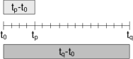
(a) $\alpha\rightarrow 0$

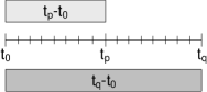
(b) $\alpha\rightarrow 0.5$

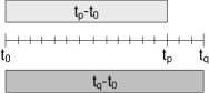
(c) $\alpha\rightarrow 1$

Figure 3: Graphical interpretation of the $\alpha$ coefficient

The second process (cf. Algorithm 6) is used for selection of circuit nodes. It utilises the information maintained by the process associated to Algorithm 4. In particular, the graph $G(V,E)$ and the labels $L(e_{ij})$ $\forall e_{ij}\in E$ are shared between both processes. When a user wants to construct a new circuit, this process is executed and it returns the nodes of the circuit. For this purpose, an exit node $x$ is chosen at random from the set of vertices $V\setminus\{s\}$. After that, the process computes until $k$ random paths of length $\delta$ between the nodes $s$ and $x$. With this aim, a recursive process, summarised in Algorithm 5, is called. In the case that there is not any path between the vertices $s$ and $x$, another exit node is chosen and the procedure is executed again. This iteration must be repeated until a) some paths of length $\delta$ between the pair of nodes $s$ and $x$ are found, or b) until a certain number of iterations are performed. In the first case, the path with the minimum latency is selected as the solution among all the obtained paths. In the second case, a completely random path of length $\delta$ is returned. To avoid this situation, i.e., to avoid that our new strategy behaves as a random selection of nodes strategy, the process associated to Algorithm 4 must be started some time before the effective establishment of circuits take place. This way, the graph $G(V,E)$ increases the necessary level of connectivity among its vertices. We refer to Section 6 for more practical details and discussions on this point.

4.1 Discussion on the adversary model

One may think that an adversary, as it was initially defined in Section 2, can try to reconstruct the client graph and guess the corresponding latency labels of our new strategy in order to degrade its anonymity degree. However, even if we assume the most extreme case, in which the adversary obtains a complementary complete graph $K_{n}$ with the set of vertices $N$ and corresponding latency labels, this does not affect the anonymity degree of our new strategy. First of all, we recall that the graph of the client is a dynamic random subgraph of $K_{n+1}$ that is evolving over time, with a set of vertices $N\cup\{s\}$. The adversary graph would also be a subgraph of $K_{n}$ with the set of vertices $N$, changing dynamically as time goes by. Therefore, the set of vertices and edges of the adversary and client graphs will never converge into same connectivity model of the network. Moreover, the latencies between the client node $s$ and any other potential entry node $e$ cannot be calculated by the adversary. Otherwise, this would mean that the anonymity has already been violated by the adversary. Indeed, the estimated latencies will definitively differ between the client and the adversary graph, since they are computed at different time frames and different source networks. Finally, the adversary also ignores the exit nodes selected by the client, as well as the $k$ parameter used by the client to choose the paths.

5 Analytical evaluation of the new strategy

We provide in this section the analytical expression of the anonymity degree of the new strategy. First, we extend the list of definitions provided in Section 2.

5.1 Analytical graph of $\psi_{grp}(N,\delta)$

In order to provide an analytical expression of the anonymity degree it is important to notice that this must be always done from the adversary standpoint. In this regard, the graph to be considered for this purpose differs with respect to the one used to compute a circuit. Note that the latencies associated to every edge which contains the client node $s$ cannot be estimated by the adversary — specially if we consider that this particular node is unknown by the adversary. Hence, an adversary aiming at violating the anonymity of client node $s$ could try to estimate the user graph without node $s$ and its associated edges. This leads us to the following definition (cf. Figure 4 as a clarifying example):

Definition 2

Given a latency graph $G(V,E)$ associated to a selection of Tor nodes $\psi_{grp}(N,\delta)$ strategy and the client node $s$, we define the analytical graph as $G^{\prime}(V^{\prime},E^{\prime})$ where $V^{\prime}=V\setminus\{s\}$ and $E^{\prime}=E\setminus\{(s,v_{i})\}$ $\forall v_{i}\in V$.

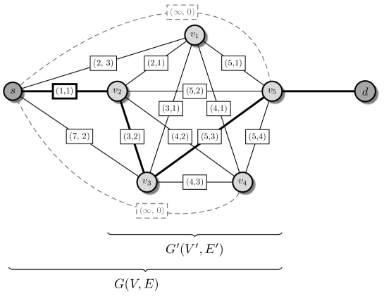
Figure 4: Example of a latency graph and its analytical graph with a selected circuit $C=\langle s,v_{2},v_{3},v_{5}\rangle$ of length $\delta=3$

5.2 $\lambda$-betweenness and $\lambda$-betweenness probability

For the purpose of computing the degree of anonymity of our new strategy, a new metric inspired by the Freeman’s betweenness centrality measure [20] is presented. This metric, called $\lambda$-betweenness, is defined as a measurement of the frequency which a node $v$ is traversed by all the possible paths of length $\lambda$ in a graph. The formal definition is given below.

Definition 3

Consider an undirected graph $G(V,E)$. Let $KP_{st}$ denote the set of paths of length $\lambda$ between a fixed source vertex $s\in V$ and a fixed target vertex $t\in V$. Let $KP_{st}(v)$ be the subset of $KP_{st}$ consisting of paths that pass through the vertex $v$. Then, we define the $\lambda$-betweenness of the node $v\in V$ as follows:

$$KP_{B}(v,\lambda)=\frac{\displaystyle\sum_{s,t\in V}\sigma_{st}(v,\lambda)}{\displaystyle\sum_{s,t\in V}\sigma_{st}(\lambda)}$$

where $\sigma_{st}(\lambda)=|KP_{st}|$ and, $\sigma_{st}(v,\lambda)=|KP_{st}(v)|$.

As we can observe, the $\lambda$-betweenness provides the proportion between the number of paths of length $\lambda$ which traverses a certain node $v$, and the number of the total paths of length $\lambda$. However, since the degree of anonymity needs a probability distribution, the following definition is required.

Definition 4

Consider an undirected graph $G(V,E)$. Let $KP_{B}(v,\lambda)$ be the $\lambda$-betweenness of the node $v\in V$. Then, the $\lambda$-betweenness probability of the node $v$ is defined as:

$$LB(v,\lambda)=\frac{KP_{B}(v,\lambda)}{\displaystyle\sum_{w\in V}KP_{B}(w,\lambda)}=\frac{\displaystyle\sum_{s,t\in V}\sigma_{st}(v,\lambda)}{\displaystyle\sum_{w\in V}\sum_{s,t\in V}\sigma_{st}(w,\lambda)}$$

It follows immediately that $0\leq LB(v,\lambda)\leq 1$, $\forall v\in V$, since this expression is equivalent to the normalised $\lambda$-betweenness.

5.3 Entropy and anonymity degree

The graph of latencies selection of Tor nodes is defined formally as an algorithm $\psi_{grp}(N,\delta)\sim f_{grp}(x)$ with an associated discrete random variable $X_{grp}$ and an analytical graph $G^{\prime}(V^{\prime},E^{\prime})$. The $\mathrm{pmf}$ $f_{grp}(x)$ is given by means of the $\lambda$-betweenness probability expression:

$$f_{grp}(x_{i})=p_{i}=\mathbb{P}(X_{grp}=x_{i})=\frac{\displaystyle\sum_{e,x\in V^{\prime}}\sigma_{ex}(v_{i},\lambda)}{\displaystyle\sum_{w\in V^{\prime}}\sum_{e,x\in V^{\prime}}\sigma_{ex}(w,\lambda)}$$

where $e$ and $x$ denotes every potential entry and exit node respectively in a Tor circuit, and $\lambda=\delta-1$. It is worth noting that the value $\lambda=\delta-1$ makes sense only if we take into consideration that the client node $s$ and its edges are removed in the analytical graph respect to the latency graph.

Hence, the entropy of a system whose clients use a graph of latencies selection of nodes strategy is:

$$H_{grp}(X)=-\displaystyle\sum_{i=1}^{n}LB(v_{i},\lambda)\cdot log_{2}\bigl{(}LB(v_{i},\lambda)\bigr{)}$$

By replacing $H_{grp}(X)$ in Equation (2), the degree of anonymity is then:

$$d_{grp}=-\displaystyle\sum_{i=1}^{n}\frac{LB(v_{i},\lambda)}{log_{2}(n)}\cdot log_{2}\bigl{(}LB(v_{i},\lambda)\bigr{)}$$

Theorem 5.1

Given a selection of Tor nodes $\psi_{grp}(N,\delta)\sim f_{grp}(x)$ with an associated discrete random variable $X_{grp}$ and an analytical graph $G^{\prime}(V^{\prime},E^{\prime})$ with $n=|V^{\prime}|$ and $m=|E^{\prime}|$, the anonymity degree is increased as the density of the analytical graph grows.

Proof

The density of a analytical graph $G^{\prime}=(V^{\prime},E^{\prime})$ measures how many edges are in the set $E^{\prime}$ compared to the maximum possible number of edges between vertices in the set $V^{\prime}$. Formally speaking, the density is given by the formula $\frac{2m}{n(n-1)}$. According to the previous expression, and since the number of nodes of the analytical graph remains constant, the only way to increase the density value is through rising the value $m$; that is, by adding new edges to the graph. Obviously, this implies that the more number of edges the analytical graph has, the more its density value is augmented.

Moreover, if we increase the density of the analytical graph by adding new edges, then the $\lambda$-betweenness probability of each vertex will be affected. In particular, the denominator of the $\lambda$-betweenness probability expression will change for all the vertices in the same manner, whereas the numerator will be increased for those vertices that lie on any new path of length $\lambda$ which contains some of the added edges. However, this increase is not arbitrary for a given vertex, since it has a maximum value determined by the total amount of paths of length $\lambda$ which traverses such vertex. Therefore, we can consider that each vertex has two states while we are adding new edges. First, a transitory state where the graph does not include all the paths of length $\lambda$ that traverse such vertex. And second, a stationary state which implies that the graph has all the paths of length $\lambda$ that traverses the given vertex. Thus, if we add new edges at random, then the numerator of the $\lambda$-betweenness probability of each vertex should be increased uniformly. Consequently, the degree of anonymity grows when the density of the graph is augmented.

It is interesting to highlight that the numerator of the $\lambda$-betweenness probability of a certain vertex will be increased while it is in a transitory state, and until the vertex achieves its stationary state. After that, such value cannot be increased. It seems obvious that the degree of anonymity associated to a particular analytical graph will be reached when all the vertices are in a stationary states; or, in other words, when it is the complete graph. Let us formalize this through the following theorem.

Theorem 5.2

Given a selection of Tor nodes $\psi_{grp}(N,\delta)\sim f_{grp}(x)$ with an associated discrete random variable $X_{grp}$ and an analytical graph $G^{\prime}(V^{\prime},E^{\prime})$ with $n=|V^{\prime}|$, the maximum anonymity degree is achieved iff $G^{\prime}(V^{\prime},E^{\prime})$ is the complete graph $K_{n}$.

Proof

($\Rightarrow$) Let us suppose that $G^{\prime}(V^{\prime},E^{\prime})$ is not the complete graph $K_{n}$. The maximum anonymity degree will be achieved when $LB(v_{i},\lambda)$ is equiprobable for all $v_{i}\in V^{\prime}$. That is:

$$\frac{\displaystyle\sum_{e,x\in V}\sigma_{ex}(v_{i},\lambda)}{\displaystyle\sum_{w\in V}\sum_{e,x\in V}\sigma_{ex}(w,\lambda)}=\frac{1}{n}~{}~{}~{}~{}~{}\forall v_{i}\in V^{\prime}$$

where $\lambda=\delta-1$, and where $e$ and $x$ represents every possible entry and exit node of a circuit respectively. The previous expression can be rewritten as follows:

$${\displaystyle\sum_{e,x\in V^{\prime}}\sigma_{ex}(v_{i},\lambda)}=\frac{\displaystyle\sum_{e,x\in V^{\prime}}\sigma_{ex}(v_{1},\lambda)+...+\sum_{e,x\in V^{\prime}}\sigma_{ex}(v_{n},\lambda)}{n}$$

Let us now suppose that the value $\sum_{e,x\in V^{\prime}}\sigma_{ex}(v_{i},\lambda)$ is fixed for every node of the analytical graph in accordance to the previous expression. Then, since $G^{\prime}(V^{\prime},E^{\prime})$ is not the complete graph $K_{n}$, we can eliminate an arbitrary edge such that the number of paths of length $\lambda$ with entry node $e$ and exit node $x$, and which traverses a given particular node $v_{j}\in V^{\prime}$, is reduced. Thus, the value of $\sum_{e,x\in V^{\prime}}\sigma_{ex}(v_{j},\lambda)$ would be affected for that given node. However, this contradicts the previous expression, since $\sum_{e,x\in V^{\prime}}\sigma_{ex}(v_{i},\lambda)$ would take different values for distinct nodes, and when such value must be the same for any node of the graph.

($\Leftarrow$) Let us suppose, by contradiction, that the maximum anonymity degree is not achieved by the analytical graph $K_{n}$ associated to $\psi_{grp}(N,\delta)$. This implies that given two different nodes $v_{j}$ and $v_{k}$ of the graph $K_{n}$, they will not have the same probability of being chosen by $\psi_{grp}(N,\delta)$; that is, $LB(v_{j},\lambda)\neq LB(v_{k},\lambda)$. Then, since $LB(v,\lambda)$ is defined as follows:

$$LB(v,\lambda)=\frac{\displaystyle\sum_{e,x\in V^{\prime}}\sigma_{ex}(v,\lambda)}{\displaystyle\sum_{w\in V^{\prime}}\sum_{e,x\in V^{\prime}}\sigma_{ex}(w,\lambda)}$$

We can consider that the only factor which makes possible the previous restriction $LB(v_{j},\lambda)\neq LB(v_{k},\lambda)$ is in the numerator, because the value of the denominator remains equal for both nodes in a fixed graph. Thus, if we want to satisfy the previous restriction, we must change the value $\sum_{e,x\in V^{\prime}}\sigma_{ex}(v,\lambda)$ of either node $v_{j}$ or node $v_{k}$. However, this is only possible if we eliminate a particular edge of the graph. This contradicts the imposed premise that the analytical graph associated to $\psi_{grp}(N,\delta)$ was the complete graph $K_{n}$.

Theorems 5.1 and 5.2 are exemplified in conjunction in Figure 5. We can observe how a density increase of an analytical graph influences in the degree of anonymity, achieving its maximum value when the graph is the complete one (i.e., it has a density equal to one).

Figure 5: Influence of the density of the analytical graph in the degree of anonymity with $|V^{\prime}|=20$ and $\delta=3$

Theorem 5.3

Let $G(V,E)$ be a undirected graph with $n=|V|$ and let $\lambda$ be a fixed length of a path, the value of $\sigma_{st}(\lambda)$ is maximised iff $G(V,E)$ is the complete graph $K_{n}$.

Proof

($\Rightarrow$) Let us suppose, by contradiction, that $G(V,E)$ is not the complete graph $K_{n}$. Then, we can choose an arbitrary edge $e_{ij}\in E$ that belongs to a path of length $\lambda$ between the nodes $s$ and $t$. Then, we can remove $e_{ij}$ from $E$ since the graph is not complete. As a consequence, the value $KP_{st}$ will be reduced. However, this contradicts the fact that the value $\sigma_{st}(\lambda)$ must be maximum since $\sigma_{st}(\lambda)=|KP_{st}|$.

($\Leftarrow$) The proof is direct, since the complete graph $K_{n}$ contains all the possible edges between its nodes, and thus $KP_{st}$ consists of all the possible paths of length $\lambda$ between the nodes $s$ and $t$.

Theorem 5.4

Let $K_{n}$ be a complete graph, the total number of paths of length $\lambda$ between any pair of vertices $s$ and $t$ is given by the expression:

$$\sum_{s,t\in V}\sigma_{st}(\lambda) =((n-1)((n-1)^{\lambda}-(-1)^{\lambda}))$$

Proof

The proof is given in Appendix 0.A.

Theorem 5.5

Given a selection of Tor nodes $\psi_{grp}(N,\delta)\sim f_{grp}(x)$ with an associated discrete random variable $X_{grp}$ and an analytical graph $G^{\prime}(V^{\prime},E^{\prime})$, the maximum anonymity degree is achieved iff

$$\sum_{e,x\in V^{\prime}}\sigma_{ex}(\lambda) =((n-1)((n-1)^{\lambda}-(-1)^{\lambda}))$$

Proof

The proof is direct by applying Theorems 5.2, 5.3 and 5.4.

6 Experimental results

We present in this section a practical implementation and evaluation of the series of strategies previously exposed. Each implementation has undergone several tests, in order to evaluate latency penalties during Web transmissions. Additionally, the degree of anonymity of every experimental test is also estimated, for the purpose of drawing a comparison among them.

Real Tor network			PlanetLab
$\#$ Nodes	Country	%	$\#$ Nodes
815	US	26.54	27
533	DE	17.36	17
187	RU	6.09	6
181	FR	5.89	6
171	NL	5.56	6
146	GB	4.75	5
132	SE	4.30	4
80	CA	2.61	3
56	AT	1.82	2
43	AU	1.40	1
40	IT	1.30	1
40	UA	1.30	1
39	CZ	1.27	1
38	CH	1.24	1
34	FI	1.11	1
34	LU	1.11	1
33	PL	1.08	1
32	JP	1.04	1
437	Others ($<$1%)	14.23	15
3071	–	100	100

Table 1: Selected PlanetLab nodes per country according to the real Tor network distribution

6.1 Node distribution and configuration in PlanetLab

In order to measure the performance of the strategies presented in our work, some practical experiments have been conducted. In particular, we deployed a private network of Tor nodes over the PlanetLab research network [21, 22]. Our deployed Tor network is composed of 100 nodes following a representative distribution based on the real (public) Tor network. We distributed the nodes of the private Tor network following the public network distribution in terms of countries and bandwidths. Table 1 summarises the distribution values per country. The estimated bandwidths of the nodes is retrieved through the directory servers of the real Tor network [23]. Then, we categorised the nodes according to their bandwidths by means of the k-means clustering methodology [24, 25]. A value of $k=100$ is used as the number of clusters (i.e., number of selected nodes in PlanetLab). When the algorithm converges, a cluster is assigned randomly to each node of the private Tor network. Subsequently, the bandwidth of each node is configured with the value of its associated centroid (i.e. the mean of the cluster). For such a purpose, the directive BandwidthRate is used in the configuration file of every node. Let us note that the country and bandwidth values are considered as independent in the final node distribution configuration. Indeed, there is no need to correlate both variables, since the bandwidth of every node can be configured by its corresponding administrator, while this fact does not depend on the country which the node belongs to.

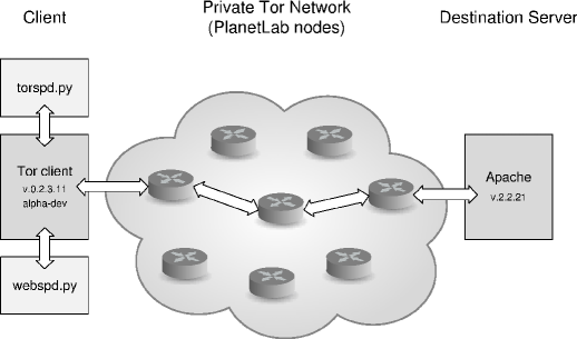
Figure 6: Conceptual representation of our testbed environment

6.2 Testbed environment

Every node of our Planetlab private network runs the Tor software, version 0.2.3.11-alpha-dev. Additionally, four nodes inside the network are configured as directory servers. These four nodes are in charge of managing the global operation of the Tor network and providing the information related to the network nodes.

(a) Web size of 50KB

(b) Web size of 150KB

(c) Web size of 320KB

Figure 7: Experimental results

Furthermore, two additional nodes outside the PlanetLab network are used in our experiments. One of them is based on an Intel Core2 Quad Processor at 2.66GHz with 6GB of RAM and a Gentoo GNU/Linux Operating System with a 3.2.9 kernel. This one is used as the client node who handles the construction of Tor circuits for every evaluated strategy. For this purpose, this node runs also our own specific software application, hereinafter denoted as torspd.py. A beta release of torspd.py, written in Python 2.6.6, can be downloaded at http://github.com/sercas/torspd. The torspd.py application relies on the TorCtl Python bindings [26] —a Tor controller software to support path building and various constraints on node and path selection, as well as statistic gathering. Moreover, torspd.py also benefits from the package NetworkX [27] for the creation, manipulation, and analysis of graphs. The client node is not only in charge of the circuit construction given a certain strategy, but also of attaching an initiated HTTP connection to an existing circuit. To accomplish this, the node uses torspd.py to connect to an special port of the local Tor software called the control port, and which allows to command the operations. The client node includes an additional software —also based on Python— capable of performing HTTP queries through our private Tor network by using a SOCKS5 connection against the local Tor client. This software, called webspd.py, is also able to obtain statistics results about the launched queries in order to evaluate the performance of the algorithms implemented in torspd.py. Finally, webspd.py performs every HTTP query making use directly of the IP address of the destination server; consequently, any perturbation introduced by a DNS resolution is avoided in our measurements. The second node outside the PlanetLab network is based on an Intel Xeon Processor at 2.00GHz with 2GB of RAM and a Debian GNU/Linux Operating System with a 2.6.26 kernel. This node is considered as the destination server, and includes an HTTP server based on Apache, version 2.2.21. The conceptual infrastructure used to carry out our experiments is illustrated in Figure 6.

With the purpose of obtaining extrapolative results, we consider in our testbed the outcomes reported in [28]. This report, based on the analysis of more than four billion Web pages, provides estimations of the average size of current Internet sites, as well as the average number of resources per page and other interesting metrics. Our testbed is built bearing in mind these premises, so that it is close enough to a real Web environment. This way, the analysed strategies (i.e., random selection, geographical selection, bandwidth selection, and graph of latencies selection) are evaluated based on three different series of experiments that vary the Web page sizes. More precisely, the client node requests via our private PlanetLab Tor network Web pages of, respectively, 50KB, 150KB and 320KB of size —being the last one the average size of a Web page according to the aforementioned report. The length of the circuits is seen as another variable in our testbed. More precisely, the different strategies are evaluated with Tor circuits of length three, four, five and six. Every experiment is repeated 100 times, from which we obtain the minimum, maximum and average time needed to download the corresponding Web pages. Likewise, the standard deviation is computed for every test. The obtained numerical results are presented in Tables 2, 3, 4 and 5, and also depicted graphically in Figure 7. In the sequel, we use these results to analyse the performance of every strategy in terms of transmission times and degree of anonymity.

6.3 Random selection of nodes strategy evaluation

As previously exposed in Theorem 3.1, the random selection of nodes strategy is the best one from the point of view of the degree of anonymity, since it achieves the maximum possible value. Nevertheless, this selection of nodes methodology suffers from an high penalty in terms of latency in accordance with the extrapolated results of our evaluation. As it can be inferred from the analysis of the numerical outcomes, and reflected in Figure 7, the random selection algorithm exhibits the worst transmission times, regardless of the size of the site or the length of the circuit used. This can be explained by the random nature of this strategy. Indeed, by selecting the nodes at random, the strategy can incur in some problems which affect directly to the latency of a computed circuit, such as a big distance between the involved nodes (in terms of countries, i.e., routers), a network congestion in a part of the circuit [29], or a selection of nodes with limited computational resources, among others. It is clear that all these drawbacks are hidden to the strategy and explain the obtained results. Moreover, all these problems are reflected in the standard deviation of the measurements, which is the higher one compared with the other alternatives.

$\psi_{rnd}(N,\delta)$, $d_{rnd}=1.0$, Web size 50KB
Circ. length	Min.	Max.	Avg.	Std. dev.
$\delta=3$	0.95094203949	3.38077807426	1.84956678152	0.58107725003
$\delta=4$	1.14792490005	7.46992301941	2.56735023022	1.03927644851
$\delta=5$	1.13161778450	12.7252390385	3.13187572718	1.69722167190
$\delta=6$	1.57145905495	14.6901309490	3.56973065615	2.06960596616
$\psi_{rnd}(N,\delta)$, $d_{rnd}=1.0$, Web size 150KB
Circ. length	Min.	Max.	Avg.	Std. dev.
$\delta=3$	0.970992088318	5.70451307297	2.46016269684	0.901269612931
$\delta=4$	1.081045866010	12.0326070786	3.34545367479	1.478886535440
$\delta=5$	1.624027013780	16.0551090240	3.78437126398	1.918732505410
$\delta=6$	2.279263019560	11.5805990696	4.71352141102	2.544477101520
$\psi_{rnd}(N,\delta)$, $d_{rnd}=1.0$, Web size 320KB
Circ. length	Min.	Max.	Avg.	Std. dev.
$\delta=3$	1.49153804779	13.2033219337	3.79921305656	2.45165379541
$\delta=4$	1.84271001816	15.2616338730	4.98011079788	2.67792560196
$\delta=5$	1.73619008064	17.1969499588	5.37626729012	3.01781647919
$\delta=6$	2.16737580299	17.8402540684	6.37420113325	3.27889183837

Table 2: Random selection of nodes strategy ($\psi_{rnd}$) results

$\psi_{geo}(N,\delta)$, $d_{geo}\approx 0.7157$, Web size 50KB
Circ. length	Min.	Max.	Avg.	Std. dev.
$\delta=3$	0.913872003555	2.36748099327	1.31694087505	0.219359721740
$\delta=4$	1.083739995960	2.03739213943	1.49165359974	0.189194613865
$\delta=5$	1.157481908800	2.17184281349	1.56993633509	0.220167861127
$\delta=6$	1.200492858890	2.63958501816	1.71368015051	0.234977785757
$\psi_{geo}(N,\delta)$, $d_{geo}\approx 0.7157$, Web size 150KB
Circ. length	Min.	Max.	Avg.	Std. dev.
$\delta=3$	1.38168692589	2.68786311150	1.79467165947	0.260276001481
$\delta=4$	1.27939105034	2.92536497116	1.87463890314	0.281488220772
$\delta=5$	1.33843898773	3.71059083939	1.98130603790	0.318113252410
$\delta=6$	1.40922594070	3.28039193153	2.05482839346	0.261217096578
$\psi_{geo}(N,\delta)$, $d_{geo}\approx 0.7157$, Web size 320KB
Circ. length	Min.	Max.	Avg.	Std. dev.
$\delta=3$	1.41799902916	2.93465995789	2.20432470083	0.310828573513
$\delta=4$	1.54156398773	3.33606600761	2.37035997391	0.329438846284
$\delta=5$	1.88031601906	4.10431504250	2.51430423737	0.370494801277
$\delta=6$	1.64570999146	3.89323496819	2.70262962818	0.376313686885

Table 3: Geographical selection strategy ($\psi_{geo}$) results

$\psi_{bw}(N,\delta)$, $d_{bw}\approx 0.9009$, Web size 50KB
Circ. length	Min.	Max.	Avg.	Std. dev.
$\delta=3$	0.964261054993	5.12318110466	1.86709306002	0.789060168081
$\delta=4$	1.078310012820	5.41474699974	2.36407416582	0.859666129425
$\delta=5$	1.060457944870	6.92380499840	2.63418945789	1.128347022810
$\delta=6$	1.278292894360	12.7536408901	3.03272451162	1.882337407440
$\psi_{bw}(N,\delta)$, $d_{bw}\approx 0.9009$, Web size 150KB
Circ. length	Min.	Max.	Avg.	Std. dev.
$\delta=3$	1.26475811005	7.09091401100	2.28234255314	0.765374484505
$\delta=4$	1.23797798157	6.80870413780	2.91089500189	0.947719280103
$\delta=5$	1.45632719994	12.6443610191	2.97445464373	1.431690789930
$\delta=6$	1.27809882164	12.7246098518	3.19875429869	1.666334473980
$\psi_{bw}(N,\delta)$, $d_{bw}\approx 0.9009$, Web size 320KB
Circ. length	Min.	Max.	Avg.	Std. dev.
$\delta=3$	1.49932813644	12.9250459671	3.29500451326	1.79104222251
$\delta=4$	1.52931094170	13.7227480412	3.70603173733	1.90767488259
$\delta=5$	1.66296601295	17.3828690052	4.07738301039	2.18405609668
$\delta=6$	2.04065585136	20.1761889458	4.32070047140	2.68160673888

Table 4: Bandwidth selection strategy ($\psi_{bw}$) results

$\psi_{grp}(N,\delta)$, $d_{grp}$ (c.f. Section 6.6), Web size 50KB
Circ. length	Min.	Max.	Avg.	Std. dev.
$\delta=3$	0.935021877289	3.61296200752	1.59488223791	0.545028374794
$\delta=4$	0.998504877090	3.74897003174	1.77225045919	0.548956074123
$\delta=5$	1.195134162900	4.21774697304	2.02931211710	0.576776679346
$\delta=6$	1.267808914180	3.35924196243	2.18245174408	0.502899662482
$\psi_{grp}(N,\delta)$, $d_{grp}$ (c.f. Section 6.6). Web size 150KB
Circ. length	Min.	Max.	Avg.	Std. dev.
$\delta=3$	1.112107038500	5.53429508209	2.04227621531	0.790901626275
$\delta=4$	1.290552854540	5.68215894699	2.66674958944	0.944641197284
$\delta=5$	1.163586854930	7.41387891769	2.68937173843	0.917799034111
$\delta=6$	1.550453186040	5.40707683563	3.00299987316	0.935654846647
$\psi_{grp}(N,\delta)$, $d_{grp}$ (c.f. Section 6.6), Web size 320KB
Circ. length	Min.	Max.	Avg.	Std. dev.
$\delta=3$	1.502956867220	7.29033994675	2.51847231626	1.009688576850
$\delta=4$	1.498482227330	6.52234792709	3.22330027342	1.061893260420
$\delta=5$	1.734797000890	6.73247194290	3.31047295094	0.940285391625
$\delta=6$	1.689666986470	7.89933013916	3.46063615084	1.094579395080

Table 5: Graph of latencies selection strategy ($\psi_{grp}$) results

6.4 Geographical selection of nodes strategy evaluation

The evaluation of the geographical selection of nodes strategy has been performed by fixing the country and taking into consideration the node distribution detailed in Table 1. United States was selected in accordance to the country where the client node resides. Therefore, we can calculate the anonymity degree for this strategy by recalling its related expression introduced in Section 3.2:

$$d_{geo}=\frac{log_{2}(m)}{log_{2}(n)}=\frac{log_{2}(27)}{log_{2}(100)}\approx 0.7157$$

As we can observe, the degree of anonymity has dropped significantly when we compare it with the results of the other strategies. However, sacrificing a certain level of anonymity incurs in a drastic fall of the latency needed to download a Web page, as it can be noticed if we compare Figures 7a, 7b and 7c. In fact, this selection of nodes methodology provides the best performance in terms of the time required to download a Web page among the other alternatives. It is also interesting to remark the fact that the standard deviation of the time measured in this method remains nearly constant regardless of the circuit length and the size of the Web page. This seems reasonable since the more geographically near are the nodes, the less random interferences affect to the whole latency. We can understand this if we think in terms of the number of networks elements (i.e., routers, switches, etc.) involved in the TCP/IP routing process between every pair of nodes. Thus, a pair of nodes which belong to the same country will be interconnected through less network elements compared to two nodes which belong to different countries and, as a consequence, the latency will be more stable along time. This can be an interesting fact, since the penalty introduced by the use of Tor affects less to the psychological perception of the user when browsing the Web [5]. Nevertheless, the anonymity degree of this strategy is strongly tied to the fixed country, since —as we pointed out in Theorem 3.3— the less nodes belonging to the country, the less anonymity degree is provided.

6.5 Bandwidth selection of nodes strategy evaluation

The anonymity degree of the bandwidth selection of nodes strategy has been computed empirically according to its associated formula (cf. Section 3.3 for details). In particular, the torspd.py application was in charge of obtaining the bandwidth of every node of our private Tor network and of calculating the anonymity degree. Thus, the anonymity degree when the evaluation of this strategy was performed was approximately 0.9009. It is important to highlight that, in spite of the fixed bandwidth specified in the configuration, the bandwidth of every onion router is estimated periodically by the Tor software running at every node, and provided later to torspd.py through the directory servers. Indeed, if we think that the established bandwidth of a node through its configuration does not necessarily correspond to the real value, then the anonymity degree can change in time in comparison to the previous strategies.

From the viewpoint of the latency results, we can observe how the bandwidth selection of nodes strategy improves the values respect to the random strategy by sacrificing some degree of anonymity. However, it does not achieve the transmission times of the geographical methodology. The reason for that is because this strategy does not take into account important networking aspects, such as network congestion, number of routers, etc., that also impact the transmission times. Therefore, it is fairly reasonable that this methodology is more susceptible to networking problems, resulting in an increase of the eventual transmission time results. This is also corroborated by the standard deviation results, noting the lack of stability of the results. In fact, the transmission times increase as the size of the Web page or the length of the circuit also increase.

6.6 Graph of latencies strategy evaluation

The experimental evaluation of our proposal has been performed after the establishment of the parameters of its related algorithms. In particular, they were $\Delta t=5$, $m=3$, $k=300$ and $max\_iter=5$. Furthermore, the Latency Computation Process was launched two hours before the execution of webspd.py, leading to an analytical graph with a set of more than 3,000 edges, and which represents a density value of, approximately, 0.67. At this moment, the torspd.py estimated the degree of anonymity in accordance to the formula presented in Section 5.3. Since such equation depends on the length of the circuit, the anonymity degree was estimated for lengths 3, 4, 5 and 6, giving the results of 0.9987, 0.9984, 0.9982 and 0.9981, respectively. As occurs with the previous strategy, the degree of anonymity is dynamic over time, and in this case depends on the connectivity of the analytical graph. Nevertheless, the anonymity degree was not estimated again during the evaluation tests.

Function $c_{t}$ was implemented by means of the construction of random circuits of length $m$. Such circuits are not used as anonymous channels for Web transmissions, but to estimate the latencies of the edges. This is possible since during the construction of a circuit, every time a new node is added to the circuit, the Latency Computation Process is notified. Hence, it is easy to determine the latency of an edge by subtracting the time instants of two nodes added consecutively to a certain circuit. Regarding this modus operandi of measuring the latencies, it is interesting to highlight two aspects. The first one is that it meets the restriction of estimating the latencies secretly; and the second one is that it not only measures the latencies in relation the network solely, but also takes into consideration delays motivated by the status of the nodes or its resources limitations. This way, our proposal models indirectly some negative issues which the other strategies do not reflect, leading to an improvement of the transmission times as the obtained results evidence.

By comparing the results of the previous strategies with the current one, we can observe how our new proposal exhibits a better trade-off between degree of anonymity and transmission latency. Particularly, from the perspective of the transmission times, our proposal is quite close to those from the geographical selection strategy, while it provides a higher degree of anonymity. Indeed, if we compare our strategy from the anonymity point of view, we can observe that only the random selection of nodes criteria overcomes our new strategy, but, as already mentioned, by sacrificing considerably the transmission time performance.

7 Related Work

The use of entropy-based metrics to measure the anonymity degree of infrastructures like Tor was simultaneously established by Diaz et al. [11] and Serjantov and Danezis [12]. Since then, several other authors have proposed alternative measures [30]. Examples include the use of the min entropy by Shmatikov and Wang in [31], and the Renyi entropy by Clauß and Schiffner in [32]. Other examples include the use of combinatorial measures by Edman et al. [33], later improved by Troncoso et al. in [34]. Snader and Borisov proposed in [35] the use of the Gini coefficient, as a way to measure inequalities in the circuit selection process of Tor. Murdoch and Watson propose in [36] to asses the bandwidth available to the adversary, and its effects to degrade the security of several path selection techniques.

With regard to literature on selection algorithms, as a way to improve the anonymity degree while also increasing performance, several strategies have been reported. Examples include the use of reputation-based strategies [37], opportunistic weighted network heuristics [35, 38], game theory [39], and system awareness [40]. Compared to those previous efforts, whose goal mainly aim at reducing overhead via bandwidth measurements while addressing the classical threat model of Tor [7], our approach takes advantage of latency measurements, in order to best balance anonymity and performance. Indeed, given that bandwidth is simply self-reported on Tor, regular nodes may be mislead and their security compromised if we allow nodes from using fraudulent bandwidth reports during the construction of Tor circuits [37, 41].

The use of latency-based measurements for path selection on anonymous infrastructures has been previously reported in the literature. In [42], Sherr et al. propose a link-based path selection strategy for onion routing, whose main criterion relies, in addition to bandwidth measures, on network link characteristics such as latency, jitter, and loss rates. This way, false perception of nodes with high bandwidth capacities is avoided, given that low-latency nodes are now discovered rather than self-advertised. Similarly, Panchenko and Renner [43] propose in their work to complement bandwidth measurements with round trip time during the construction of Tor circuits. Their work is complemented by practical evaluations over the real Tor network and demonstrate the improvement of performance that such latency-based strategies achieve. Finally, Wang et al. [44, 45] propose the use of latency in order to detect and prevent congested nodes, so that nodes using the Tor infrastructure avoid routing their traffic over congested paths. In contrast to these proposals, our work aims at providing a defence mechanism. Our latency-based approach is considered from a node-centred perspective, rather than a network-based property used to balance transmission delays. This way, adversarial nodes are prevented from increasing their chances of relying traffic by simply presenting themselves as low-latency nodes, while guaranteeing an optimal propagation rate by the remainder nodes of the system.

8 Conclusion

We addressed in this paper the influence of circuit construction strategies on the anonymity degree of the Tor (The onion router) anonymity infrastructure. We evaluated three classical strategies, with respect to their de-anonymisation risk and latency, and regarding its performance for anonymising Internet traffic. We then presented the construction of a new circuit selection algorithm that considerably reduces the success probability of linking attacks while providing enough performance for low-latency services. Our experimental results, conducted on a real-world Tor deployment over PlanetLab confirm the validity of the new strategy, and shows that it overperforms the classical ones.

Appendix 0.A Number of walks of length $\lambda$ between any two distinct vertices of a $K_{n}$ graph

Let $K_{n}$ be a complete graph with $n$ vertices and $\frac{n(n-1)}{2}$ edges, such that every pair of distinct vertices is connected by a unique edge. Then, a walk in $K_{n}$ of length $\lambda$ from vertex $v_{1}$ to vertex $v_{\lambda+1}$ corresponds to the following sequence:

$\underbrace{v_{1}\xrightarrow{e_{1}}v_{2}\xrightarrow{e_{2}}v_{3}\xrightarrow{e_{3}}v_{4}\xrightarrow{e_{4}}...\xrightarrow{e_{\lambda-1}}v_{\lambda}\xrightarrow{e_{\lambda}}v_{\lambda+1}}_{\text{walk in G of length $\lambda$}}$

such that each $v_{i}$ is a vertex of $K_{n}$, each $e_{j}$ is an edge of $K_{n}$, and the vertices connected by $e_{i}$ are $v_{i}$ and $v_{i+1}$.

Let $A$ be the adjacency matrix of $K_{n}$, such that $A$ is an $n$-square binary matrix in which each entry is either zero or one, i.e., every $(i,j)$-entry in $A$ is equal to the number of edges incident to $v_{i}$ and $v_{j}$. Moreover, $A$ is symmetric and circulant [46]. It has always zeros on the leading diagonal and ones off the leading diagonal. For example, the adjacency matrix of a complete graph $K_{4}$ is always equal to:

$$A=\begin{bmatrix}0&1&1&1\\ 1&0&1&1\\ 1&1&0&1\\ 1&1&1&0\\ \end{bmatrix}$$

The total number of possible walks of length $\lambda$ from vertex $v_{i}$ to vertex $v_{j}$ is the $(i,j)$-entry of $A^{\lambda}$, i.e., the matrix product, denoted by ($\cdot$), of $\lambda$ copies of $A$ [47]. Following the above example, the number of walks of length $2$ between any two distinct vertices can be obtained directly from $A^{2}$, such that

$$A^{2}=A\cdot A=\begin{bmatrix}(n-1)&(n-2)&(n-2)&(n-2)\\ (n-2)&(n-1)&(n-2)&(n-2)\\ (n-2)&(n-2)&(n-1)&(n-2)\\ (n-2)&(n-2)&(n-2)&(n-1)\\ \end{bmatrix}$$

which leads to

$$A^{2}=A\cdot A=\begin{bmatrix}3&2&2&2\\ 2&3&2&2\\ 2&2&3&2\\ 2&2&2&3\\ \end{bmatrix}$$

Note that any $(i,j)$-entry of $A^{2}$ (where $i\neq j$) gives the same number of walks of length $2$ from any two distinct vertex $v_{i}$ to vertex $v_{j}$. The total number of walks of length $2$ between any two distinct vertices can, thus, be obtained by consecutively adding the values of every $(i,j)$-entry off the leading diagonal of matrix $A^{2}$. In the above example, it suffices to sum $(4(4-1))$ times (i.e., twice the number of edges in $K_{4}$) the value $2$ that any $(i,j)$-entry (where $i\neq j$) has in $A^{2}$. This amounts to having exactly $24$ possible walks on any $K_{4}$ graph.

Therefore, the problem of finding the number of walks of length $\lambda$ between any two distinct vertices of a $K_{n}$ graph reduces to finding the $(i,j)$-entry of $A^{\lambda}$, where $i\neq j$. Indeed, let $a^{\lambda}_{i,j}$ be the $(i,j)$-entry of $A^{\lambda}$. Then, the recurrence relation between the original adjacency matrix $A$, and the matrix product of up to $\lambda-1$ copies of $A$, i.e.,

$$A^{\lambda}=A^{\lambda-1}\cdot A$$ (3)

with initial conditions:
$$a^{2}_{i,j}=\left\{\begin{array}[]{ll}(n-2)&\text{if}~{}~{}i\neq j\\ (n-1)&\text{if}~{}~{}i=j\end{array},\right.$$ $$a^{1}_{i,j}=\left\{\begin{array}[]{ll}1&\text{if}~{}~{}i\neq j\\ 0&\text{if}~{}~{}i=j\end{array}\right.$$

is sufficient to solve the problem. Notice, moreover, that the result does not depend on any precise value of either $i$ or $j$. Indeed, it is proved in [47] that there is a constant relationship between the $(i,j)$-entries off the leading diagonal of $A^{\lambda}$ and the $(i,j)$-entries on the leading diagonal of $A^{\lambda}$. More precisely, let $t^{\lambda}$ be any $(i,j)$-entry off the leading diagonal of $A^{\lambda}$ (i.e., $t^{\lambda}=a^{\lambda}_{i,j}$ such that $i\neq j$). Let $d^{\lambda}$ be any $(i,i)$-entry on the leading diagonal of $A^{\lambda}$ (i.e., $t^{\lambda}=a^{\lambda}_{i,i}$). Then, if we subtract $t^{\lambda}$ from $d^{\lambda}$, the results is always equal to $(-1)^{\lambda}$. In other words, if we express $A^{\lambda}$ as follows:

$$A^{\lambda}=[a^{\lambda}_{i,j}]=\left\{\begin{array}[]{ll}t^{\lambda}&\text{if}~{}~{}i\neq j\\ d^{\lambda}&\text{if}~{}~{}i=j\end{array}\right.$$

then $t^{\lambda}=d^{\lambda}+(-1)^{\lambda}$. We can now use the recurrence relation shown in Equation (3) to derive the following two results:

$$t^{\lambda} = (n-2)t^{\lambda-1}+d^{\lambda-1}$$ (4)

$$d^{\lambda} = (n-1)t^{\lambda-1}$$ (5)

with the initial conditions $t^{1}=1$ and $d^{1}=0$.

Cumbersome, but elementary, transformations shown in both [46] and [47] lead us to unfold the two recurrence relations in both Equation (4) and (5) to the following two self-contained expressions:

$$t^{\lambda} = \frac{(n-1)^{\lambda}-(-1)^{\lambda}}{n}$$ (6)

$$d^{\lambda} = \frac{(n-1)^{\lambda}+(n-1)(-1)^{\lambda}}{n}$$ (7)

To conclude, we can now use Equations (6) and (7) to express the total number of closed and non-closed walks in the complete graph $K_{n}$ by simply adding to them twice the number of edges in the graph, i.e., $n(n-1)$. From Equation (6) we have now the value of any $(i,j)$-entry in $A^{\lambda}$ such that $i\neq j$. As we did previously in the example of the complete graph $K_{4}$, the total number of walks of length $\lambda$ between any two distinct vertices can be obtained by consecutively adding $n(n-1)$ times the values of any of the $(i,j)$-entries off the leading diagonal of matrix $A^{\lambda}$. This amounts to having exactly $n(n-1)\cdot t^{\lambda}$ which simplifying leads to:

$$((n-1)((n-1)^{\lambda}-(-1)^{\lambda}))$$ (8)

possible walks of length $\lambda$ on any $K_{n}$ graph.

References

- [1] C. Troncoso, E. Costa-Montenegro, C. Diaz, S. Schiffner, On the Difficulty of Achieving Anonymity for Vehicle-2-X Communication, Computer Networks 55 (14) (2011) 3199–3210. doi:10.1016/j.comnet.2011.05.004.
- [2] N. Bansod, A. Malgi, B. K. Choi, J. Mayo, MuON: Epidemic Based Mutual Anonymity in Unstructured P2P Networks, Computer Networks 52 (5) (2008) 915–934. doi:10.1016/j.comnet.2007.11.011.
- [3] P. F. Syverson, D. M. Goldschlag, M. G. Reed, Anonymous Connections and Onion Routing, in: Proceedings of the 1997 IEEE Symposium on Security and Privacy, SP’97, IEEE Computer Society, Washington, DC, USA, 1997, pp. 44–54.
- [4] R. Dingledine, N. Mathewson, P. Syverson, Tor: The Second-generation Onion Router, in: Proceedings of the 13th conference on USENIX Security Symposium - Volume 13, SSYM’04, USENIX Association, Berkeley, CA, USA, 2004, pp. 21–21.
- [5] S. Köpsell, Low Latency Anonymous Communication – How Long Are Users Willing to Wait?, in: G. Müller (Ed.), Emerging Trends in Information and Communication Security, Vol. 3995 of Lecture Notes in Computer Science, Springer Berlin / Heidelberg, 2006, pp. 221–237. doi:10.1007/11766155_16.
- [6] X. León, T. A. Trinh, L. Navarro, Modeling Resource Usage in Planetary-Scale Shared Infrastructures: PlanetLab’s Case Study, Computer Networks 55 (15) (2011) 3394–3407. doi:10.1016/j.comnet.2011.06.026.
- [7] P. Syverson, G. Tsudik, M. Reed, C. Landwehr, Towards an Analysis of Onion Routing Security, in: International workshop on Designing privacy enhancing technologies: design issues in anonymity and unobservability, Springer-Verlag New York, Inc., New York, NY, USA, 2001, pp. 96–114.
- [8] N. Hopper, E. Y. Vasserman, E. Chan-TIN, How Much Anonymity does Network Latency Leak?, ACM Transactions on Information and System Security (TISSEC) 13 (2) (2010) 13:1–13:28. doi:10.1145/1698750.1698753.
- [9] A. Back, U. Möller, A. Stiglic, Traffic Analysis Attacks and Trade-Offs in Anonymity Providing Systems, in: Proceedings of the 4th International Workshop on Information Hiding, IHW’01, Springer-Verlag, London, UK, UK, 2001, pp. 245–257.
- [10] S. J. Murdoch, Hot or Not: Revealing Hidden Services by Their Clock Skew, in: Proceedings of the 13th ACM conference on Computer and communications security, CCS’06, ACM, New York, NY, USA, 2006, pp. 27–36. doi:10.1145/1180405.1180410.
- [11] C. Díaz, S. Seys, J. Claessens, B. Preneel, Towards Measuring Anonymity, in: Proceedings of the 2nd international conference on Privacy enhancing technologies, PET’02, Springer-Verlag, Berlin, Heidelberg, 2003, pp. 54–68.
- [12] A. Serjantov, G. Danezis, Towards an Information Theoretic Metric for Anonymity, in: Proceedings of the 2nd international conference on Privacy enhancing technologies, PET’02, Springer-Verlag, Berlin, Heidelberg, 2003, pp. 41–53.
- [13] J. A. Tomlin, An Entropy Approach to Unintrusive Targeted Advertising on the Web, Computer Networks 33 (1-6) (2000) 767–774. doi:10.1016/S1389-1286(00)00062-1.
- [14] Y. Jiang, Y. Fan, X. (Sherman) Shen, C. Lin, A Self-adaptive Probabilistic Packet Filtering Scheme Against Entropy Attacks in Network Coding, Computer Networks 53 (18) (2009) 3089–3101. doi:10.1016/j.comnet.2009.08.002.
- [15] B. Tellenbach, M. Burkhart, D. Schatzmann, D. Gugelmann, D. Sornette, Accurate Network Anomaly Classification With Generalized Entropy Metrics, Computer Networks 55 (15) (2011) 3485–3502. doi:10.1016/j.comnet.2011.07.008.
- [16] Z. Dong, R. D. W. Perera, R. Chandramouli, K. P. Subbalakshmi, Network Measurement Based Modeling and Optimization for IP Geolocation, Computer Networks 56 (1) (2012) 85–98. doi:10.1016/j.comnet.2011.08.011.
- [17] S. Crisóstomo, U. Schilcher, C. Bettstetter, J. a. Barros, Probabilistic Flooding in Stochastic Networks: Analysis of Global Information Outreach, Computer Networks 56 (1) (2012) 142–156. doi:10.1016/j.comnet.2011.08.014.
- [18] M. Coates, A. Hero, R. Nowak, B. Yu, Internet Tomography, Signal Processing Magazine, IEEE 19 (3) (2002) 47–65. doi:10.1109/79.998081.
- [19] J. Hunter, The Exponentially Weighted Moving Average, Journal of Quality Technology 18 (4) (1986) 203–210.
- [20] L. C. Freeman, A Set of Measures of Centrality Based on Betweenness, Sociometry 40 (1) (1977) 35–41.
- [21] B. Chun, D. Culler, T. Roscoe, A. Bavier, L. Peterson, M. Wawrzoniak, M. Bowman, PlanetLab: An Overlay Testbed for Broad-Coverage Services, ACM SIGCOMM Computer Communication Review 33 (3). doi:10.1145/956993.956995.
- [22] L. Peterson, S. Muir, T. Roscoe, A. Klingaman, PlanetLab Architecture: An Overview, Tech. Rep. PDN–06–031, PlanetLab Consortium (May 2006).
-
[23]
R. Dingledine, M. Perry, N. Mathewson, D. Johnson, D. Fifield, G. Kadianakis,
J. Appelbaum, K. Loesing, L. Nordberg, R. Ransom, S. Hahn,
Tor directory protocol, version 3 (2005-2012).
URL https://gitweb.torproject.org/torspec.git/blob_plain/HE%%****␣main.tex␣Line␣2200␣****AD:/dir-spec.txt - [24] J. MacQueen, Some Methods for Classification and Analysis of Multivariate Observations, in: Proceedings of the 5th Berkeley symposium on mathematical statistics and probability, Vol. 1, California, USA, 1967, p. 14.
- [25] M. Anderberg, Cluster Analysis for Applications, Tech. rep., DTIC Document, Academic Press (1973).
-
[26]
N. Mathewson, R. Dingledine, M. Perry, D. Johnson, H. Bock, T. Touceda,
Python Tor
controller (2005-2011).
URL https://gitweb.torproject.org/atagar/pytorctl.git - [27] A. A. Hagberg, D. A. Schult, P. J. Swart, Exploring Network Structure, Dynamics, and Function Using NetworkX, in: Proceedings of the 7th Python in Science Conference (SciPy2008), Pasadena, CA USA, 2008, pp. 11–15.
-
[28]
S. Ramachandran,
Web metrics:
Size and number of resources (May 2010).
URL https://developers.google.com/speed/articles/web-metric%s - [29] H. Bai, M. Chen, CCIPCA-OPCSC: An Online Method for Detecting Shared Congestion Paths, Computer Networks 56 (1) (2012) 399–411. doi:10.1016/j.comnet.2011.09.016.
- [30] A. Hamel, J. Grégoire, I. Goldberg, The Mis-entropists: New Approaches to Measures in Tor, Tech. Rep. 18, University of Waterloo (2011).
- [31] V. Shmatikov, M.-H. Wang, Measuring Relationship Anonymity in Mix Networks, in: Proceedings of the 5th ACM workshop on Privacy in electronic society, WPES’06, ACM, New York, NY, USA, 2006, pp. 59–62. doi:10.1145/1179601.1179611.
- [32] S. Clauß, S. Schiffner, Structuring Anonymity Metrics, in: Proceedings of the second ACM workshop on Digital identity management, ACM, 2006, pp. 55–62. doi:10.1145/1179529.1179539.
- [33] M. Edman, F. Sivrikaya, B. Yener, A Combinatorial Approach to Measuring Anonymity, in: Intelligence and Security Informatics, 2007 IEEE, IEEE, 2007, pp. 356–363. doi:10.1109/ISI.2007.379497.
- [34] C. Troncoso, B. Gierlichs, B. Preneel, I. Verbauwhede, Perfect Matching Disclosure Attacks, in: Proceedings of the 8th international symposium on Privacy Enhancing Technologies, PETS’08, Springer-Verlag, Berlin, Heidelberg, 2008, pp. 2–23. doi:10.1007/978-3-540-70630-4_2.
- [35] R. Snader, N. Borisov, A Tune-up for Tor: Improving Security and Performance in the Tor Network, in: Network and Distributed Security Symposium (NDSS 2008), Vol. 8, Internet Society, 2008.
- [36] S. J. Murdoch, R. N. Watson, Metrics for Security and Performance in Low-Latency Anonymity Systems, in: Proceedings of the 8th International Symposium on Privacy Enhancing Technologies, PETS’08, Springer-Verlag, Berlin, Heidelberg, 2008, pp. 115–132. doi:10.1007/978-3-540-70630-4_8.
- [37] K. Bauer, D. McCoy, D. Grunwald, T. Kohno, D. Sicker, Low-Resource Routing Attacks Against Tor, in: 2007 ACM workshop on Privacy in electronic society (WPES’07), ACM, New York, NY, USA, 2007, pp. 11–20. doi:10.1145/1314333.1314336.
- [38] R. Snader, N. Borisov, EigenSpeed: Secure Peer-to-peer Bandwidth Evaluation, in: Proceedings of the 8th international conference on Peer-to-peer systems, IPTPS’09, USENIX Association, Berkeley, CA, USA, 2009, pp. 9–9.
- [39] N. Zhang, W. Yu, X. Fu, S. Das, gPath: A Game-Theoretic Path Selection Algorithm to Protect Tor’s Anonymity, in: T. Alpcan, L. Buttyán, J. Baras (Eds.), Decision and Game Theory for Security, Vol. 6442 of Lecture Notes in Computer Science, Springer Berlin / Heidelberg, 2010, pp. 58–71. doi:10.1007/978-3-642-17197-0_4.
- [40] M. Edman, P. Syverson, As-awareness in Tor Path Selection, in: Proceedings of the 16th ACM conference on Computer and communications security, CCS’09, ACM, New York, NY, USA, 2009, pp. 380–389. doi:10.1145/1653662.1653708.
- [41] J. Garcia-Alfaro, M. Barbeau, E. Kranakis, Evaluation of Anonymized ONS Queries, in: Workshop on Security of Autonomous and Spontaneous Networks (SETOP 2008), 2008, pp. 47–60.
- [42] M. Sherr, M. Blaze, B. T. Loo, Scalable Link-Based Relay Selection for Anonymous Routing, in: Proceedings of the 9th International Symposium on Privacy Enhancing Technologies, PETS’09, Springer-Verlag, Berlin, Heidelberg, 2009, pp. 73–93. doi:10.1007/978-3-642-03168-7_5.
- [43] A. Panchenko, J. Renner, Path Selection Metrics for Performance-Improved Onion Routing, in: 9th Annual International Symposium on Applications and the Internet (SAINT’09), IEEE, 2009, pp. 114–120. doi:10.1109/SAINT.2009.26.
- [44] T. Wang, K. Bauer, C. Forero, I. Goldberg, Congestion-aware Path Selection for Tor, Tech. Rep. 20, University of Waterloo (2011).
- [45] T. Wang, K. Bauer, C. Forero, I. Goldberg, Congestion-aware Path Selection for Tor, in: 16th International Conference on Financial Cryptography and Data Security (FC’12), 2012.
- [46] P. Barry, On Integer Sequences Associated with the Cyclic and Complete Graphs, Journal of Integer Sequences 10, article 07.4.8.
- [47] R. P. Stanley, Topics in Algebraic Combinatorics, course notes for Mathematics 192 (Algebraic Combinatorics), Harvard University, Cambridge U.S.A. (2000).