Sensory organ like response determines the magnetism of zigzag-edged honeycomb nanoribbons

Abstract

We present an analytical theory for the magnetic phase diagram for zigzag edge terminated honeycomb nanoribbons described by a Hubbard model with an interaction parameter $U$. We show that the edge magnetic moment varies as $\ln{U}$ and uncover its dependence on the width $W$ of the ribbon. The physics of this owes its origin to the sensory organ like response of the nanoribbons, demonstrating that considerations beyond the usual Stoner-Landau theory are necessary to understand the magnetism of these systems. A first order magnetic transition from an anti-parallel orientation of the moments on opposite edges to a parallel orientation occurs upon doping with holes or electrons. The critical doping for this transition is shown to depend inversely on the width of the ribbon. Using variational Monte-Carlo calculations, we show that magnetism is robust to fluctuations. Additionally, we show that the magnetic phase diagram is generic to zigzag edge terminated nanostructures such as nanodots. Furthermore, we perform first principles modeling to show how such magnetic transitions can be realized in substituted graphene nanoribbons.

Interest and activity in magnetic nanostructures has been driven by their possible application in nanoelectronic/spintronic devices, with graphene based systems grabbing a significant fraction of the attention.Westervelt (2008) The remarkable electronic properties of grapheneNeto et al. (2009); Pati et al. (2011) with a Dirac like spectrum have made it a suitable candidate for many applications.Bunch et al. (2005); Miao et al. (2007); Ponomarenko et al. (2008); Wurm et al. (2009) From a theoretical perspective, electron interactions and correlations effects on the honeycomb lattice contain many interesting phenomenaKotov et al. (2010) including magnetismMeng et al. (2010) and superconductivity.Pathak et al. (2010)

Magnetism at the zigzag terminated edges of graphene has been studied by first principles calculationsSon et al. (2006a, b), and by a simplified effective Hubbard model Peres et al. (2004); Fernandez-Rossier and Palacios (2007); Bhowmick and Shenoy (2008); Yazyev (2008); Jung and MacDonald (2009); Ma et al. (2010); Yazyev (2010) described by a hopping parameter $t$ and a site-local repulsion $U$. Ref. Bhowmick and Shenoy, 2008 showed that the magnetism in graphene is robust to “shape disorder” of the nanostructure, while ref. Jung and MacDonald, 2009 studied finite width graphene nanoribbons including the effects of doping. There are also studies of defect induced magnetismZhang et al. (2007); Yazyev and Helm (2007) and of magnetism of other nanostructuresEzawa (2007); Fernandez-Rossier and Palacios (2007). There are encouraging recent experimental signatures of magnetismRamakrishna Matte et al. (2009); Rao et al. (2012); Joly et al. (2010), along with suggestionsKunstmann et al. (2011) that extraneous effects such as reconstruction would render the magnetism fragile.

The origin of magnetic moment in zigzag edge terminated honeycomb nanostructures has been attributed to the edge statesNakada et al. (1996); Wakabayashi et al. (1999); Neto et al. (2009) - localized electronic states which have most weight at the edges and die exponentially in the bulk.Brey and Fertig (2006a, b); Zarea and Sandler (2009) These states are of topological originRyu and Hatsugai (2002) and have been experimentally observed using scanning tunneling microscopy.Kobayashi et al. (2005); Niimi et al. (2006) Magnetism at the edges is attributed to the Stoner mechanism(see, e.g., Altland and Simons (2006)) and is best discussed in terms of a Landau theory.Altland and Simons (2006) The ground state energy of the system is expressed as

$$E(\mbox{\boldmath$M$})=a(U_{c}-U)|\mbox{\boldmath$M$}|^{2}+b|\mbox{\boldmath$M$}|^{4}+\ldots$$ (1)

where $M$ is the magnetic order parameter, $a,b>0$ are positive constants that depend on the microscopics, and $U_{c}$ is a critical value of the on-site repulsion. For $U<U_{c}$, the energy is minimum when $\mbox{\boldmath$M$}=\mbox{\boldmath$0$}$, i. e., system is non-magnetic. At $U=U_{c}$, there is a quantum phase transition to the magnetic state, and for $U>U_{c}$ one finds $|\mbox{\boldmath$M$}|\sim\sqrt{U-U_{c}}$. Stoner theoryYosida (1996), based on linear response formulation, provides an expression for $U_{c}\sim\frac{1}{g(\varepsilon_{F})}$, where $g(\varepsilon_{F})$ is density of states of the bare system ($U=0$) at the zero temperature chemical potential $\varepsilon_{F}$. Thus for a zigzag edge terminated system, $U_{c}$ would vanish, since the density of states $g(\varepsilon_{F})$ diverges owing to the non dispersive nature of the edge states. The Stoner-Landau theory would therefore suggest that a zigzag edge will have spontaneous magnetization $M$ for any $U>0$, and furthermore that $|\mbox{\boldmath$M$}|\sim\sqrt{U}$ for $U\ll t$.

It is knownBhowmick and Shenoy (2010) that a zigzag edge terminated nanoribbon has a highly nonlinear response akin to that of sensory organs like eyes and ears. Their density response depends logarithmically on the magnitude of an edge potential applied at the zigzag edges. In this paper we show that such a Weber-Fechner response of these nanoribbons plays a central role in determining their magnetism. Our work leads to a “magnetic phase diagram” of lightly doped nanoribbons, including analytical expressions for the width $W$ and $U$ dependence of the magnetization, excitation gap, and the critical doping required to engender magnetic transitions. We also corroborate these results with variational quantum Monte Carlo calculations and show that the magnetism is robust to fluctuations. To the best of our knowledge, this is the first report that clearly points out that the usual Stoner-Landau theory is inadequate to understand magnetism of hexagonal lattice nanoribbons. This gains added significance in view of recent developments of cold atom optical lattices,I. Bloch et al. (2012) where honeycomb lattices have been realized and studied.Tarruell et al. (2012)

The simplest Hamiltonian that describes the energetics of interacting electrons in the honeycomb lattice is the Hubbard model

$$H=-t\sum_{\langle ij\rangle,\sigma}c^{\dagger}_{i\sigma}c_{j\sigma}+Ue_{0}\sum_{i}n_{i\uparrow}n_{i\downarrow}-\mu\sum_{i}n_{i\sigma}$$ (2)

where $c^{\dagger}_{i\sigma}$ is the operator that creates an electron of spin $\sigma$ at site $i$, $n_{i\sigma}=c^{\dagger}_{i\sigma}c_{i\sigma}$ is the number operator, $t$ is the nearest neighbour hopping amplitude, $Ue_{0}$ is the on-site Hubbard repulsion ($e_{0}=\frac{\sqrt{3}}{2}t$ is a characteristic energy scale, $U$ is dimensionless), and $\mu$ is the chemical potential. The underlying triangular Bravais lattice has a lattice parameter $a$, and the width of the the zigzag edge terminated nanoribbon is denoted by $W$.

  

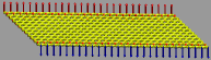
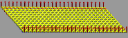
(a)                                        (b)

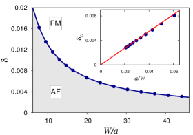
(c)

Figure 1: (color online) Two possible magnetic states of zigzag-edged nanoribbon, (a) antiferromagnetic (AF) and (b) ferromagnetic (FM). (c) Magnetic phase diagram of zigzag nanoribbons for $U=1.5$ obtained from numerical mean field calculations. Inset: the critical doping required for AF to FM transition is inversely proportional to the ribbon width.

Ground state of the zigzag edge terminated ribbon is obtained by a mean field analysis, where the four fermion interaction term is treated in the “magnetic channel” via the ansatz $n_{i\uparrow}n_{i\downarrow}\rightarrow\frac{1}{2}N_{i}\sum_{\sigma}n_{i\sigma}+M_{i}S^{z}_{i}-\left(\frac{1}{4}N_{i}^{2}-M_{i}^{2}\right)$, where $S^{z}_{i}=\frac{1}{2}\left(n_{i\uparrow}-n_{i\downarrow}\right)$, $N_{i}=\langle\sum_{\sigma}n_{i\sigma}\rangle$ is the mean occupancy, and $M_{i}=\langle S^{z}_{i}\rangle$ is the local magnetization at site $i$. The quantities $N_{i}$ and $M_{i}$ are to be determined by enforcing the self consistency conditions of the mean field theory. Our detailed numerical calculation exploits translational symmetry along the nanoribbon (see Fig. 1(a)) where we have used up to 4000 equally spaced points to sample the 1D Brillouin zone. Fig. 1 shows the results for the values of physical parameters typical for graphene. We find that there are two possible magnetic configurations where the moments along the two edges of nanoribbon are oppositely aligned (the anti-ferro (AF) configuration, see Fig. 1(a)) and aligned in the same direction (the ferro (FM) configuration, see Fig. 1(b)). For both these configurations, the moments are concentrated on the sites at the edge layers – this point will be important in the discussion below. At half-filling (one electron per site), the ground state has an AF structure consistent with earlier resultsSon et al. (2006a). With the doping of holes denoted by $\delta$ ($\delta$ is defined as the doping per edge atom of the ribbon), the ground state changes to the FM configuration at a critical dopingJung and MacDonald (2009). This critical doping $\delta_{c}$ required for the first order transition is dependent on the width of the ribbon and we find that $\delta_{c}\sim\frac{a}{W}$ as shown in Fig. 1(c), the “magnetic phase diagram”. In the remainder of the paper, we develop an analytical theory of the physics behind this phase diagram.

The continuum field theoryHerbut (2006) that captures the physics of the Hamiltonian eqn. (2) has the action ($\hbar=1$)

$$\begin{split}{\cal S}[\Psi]&=\int\mbox{d}{{}^{2+1}r}\,\,\,\sum_{\sigma}\Psi^{\star}_{\sigma}(r)\left(\mathds{1}\partial_{\tau}+{\cal H}_{K}\right)\Psi_{\sigma}(r)\\ &+Ue_{0}a^{2}\int\mbox{d}{{}^{2+1}r}\left[\frac{1}{4}n(r)^{2}-\{s^{z}(r)\}^{2}\right]\end{split}$$ (3)

where $r=(\boldsymbol{r},\tau)$, $\boldsymbol{r}\equiv(x,y)$ is the position vector where $x$-coordinate is along the length of the ribbon and $y$ along the width, $\tau$ is the imaginary time that runs from $0$ to $\beta$ (inverse temperature), $\Psi^{\star}_{\sigma}=\left(\psi^{\star}_{A+\sigma}\,\,\psi^{\star}_{B+\sigma}\,\,\psi^{\star}_{A-\sigma}\,\,\psi^{\star}_{B-\sigma}\right)$ is the array of Grassmann fields with $A/B$ and $+/-$ being, respectively, sublattice and valley indices, $n(r)=\sum_{a\nu\sigma}\psi^{\star}_{a\nu\sigma}(r)\psi_{a\nu\sigma}(r)$ is the number density, $s^{z}(r)=\frac{1}{2}\sum_{a\nu\sigma}\sigma\psi^{\star}_{a\nu\sigma}(r)\psi_{a\nu\sigma}(r)$ is the spin density, $\mathds{1}$ is the $4\times 4$ identity matrix, and

$${\cal H}_{K}=v_{F}\left(\begin{array}[]{cc}\mbox{\boldmath$\tau$}\cdot\mbox{\boldmath$P$}&\mbox{\boldmath$0$}\\ \mbox{\boldmath$0$}&-\mbox{\boldmath$\tau$}^{*}\cdot\mbox{\boldmath$P$}\\ \end{array}\right)-\mu\mathds{1}$$ (4)

with $v_{F}=e_{0}a$, and $\mbox{\boldmath$P$}=-i\mbox{\boldmath$\nabla$}$, the momentum operator, $\mbox{\boldmath$\tau$}=\tau_{x}\mbox{\boldmath$e$}_{x}+\tau_{y}\mbox{\boldmath$e$}_{y}$ ($\tau_{x,y}$ – Pauli matrices in the sublattice space, $\mbox{\boldmath$e$}_{x,y}$ are spatial basis vectors). The action, written in a form that anticipates magnetism, can be studied by introducing a Hubbard-Stratanovich field $m(r)$ to decouple the $(s^{z})^{2}$ term in eqn. (3), while the $n^{2}$ term can be treated in a straightforward manner via a Hartree shift. The action becomes

$$\begin{split}{\cal S}[\Psi,m]&=\int\mbox{d}{{}^{2+1}r}\sum_{\sigma}\Psi^{\star}_{\sigma}(r)\left(\mathds{1}\partial_{\tau}+{\cal H}_{K}\right)\Psi_{\sigma}(r)\\ &+\int\mbox{d}{{}^{2+1}r}\left[m(r)s^{z}(r)+\mbox{g.c.}+\frac{1}{Ue_{0}a^{2}}|m(r)|^{2}\right]\end{split}$$ (5)

which upon integration of the fermion fields yields

$${\cal S}[m]=\ln{\prod_{\sigma}\det\left(-G^{-1}_{\sigma}[m]\right)}+\frac{1}{Ue_{0}a^{2}}\int\mbox{d}{{}^{2+1}r}|m(r)|^{2},$$ (6)

where the inverse Green’s function is given by $-G^{-1}_{\sigma}(r,r^{\prime},m)=\left[\mathds{1}\partial_{\tau}+{\cal H}_{K}+\frac{\sigma}{2}\{m(r)+m^{*}(r)\}\mathds{1}\right]\delta(r-r^{\prime})$. The magnetic ground state of the system can be described by a saddle point of the action eqn. (6). The saddle point field $m_{s}$ satisfies the condition

$$\frac{1}{Ue_{0}a^{2}}m_{s}(r)=\sum_{\sigma}\frac{\sigma}{2}G_{\sigma}(r,r;m_{s}).$$ (7)

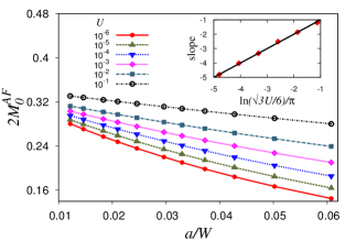
Figure 2: (color online) (a) Width dependence of magnetic moment of the AF configuration for different values of $U$ obtained from the full numerical solution compared with the analytical result eqn. (11). Inset: The logarithmic dependence of the slope of $M^{AF}_{0}$ vs. $a/W$ on $U$ – points are obtained from the numerical simulations, solid line is from eqn. (11).

We consider two different saddle point ansatzes for the undoped nanoribbons. For the AF configuration, we have

$$m_{s}^{AF}(y)=Ue_{0}a^{2}\left[\frac{M^{AF}}{a}\delta_{D}(y-W)-\frac{M^{AF}}{a}\delta_{D}(y)\right]$$ (8)

where $M^{AF}$ is the moment associated with one edge, and FM configuration has

$$m_{s}^{FM}(y)=Ue_{0}a^{2}\left[\frac{M^{FM}}{a}\delta_{D}(y-W)+\frac{M^{FM}}{a}\delta_{D}(y)\right],$$ (9)

where $M^{FM}$ is, again, the moment associated with one edge, and $\delta_{D}$ is the Dirac delta function. Solution of $M^{AF}$ and $M^{FM}$ is aided by the observation that the right hand side of eqn. (7) is the magnetic moment density response of a nanoribbon with applied edge Zeeman fields. As shown in ref. Bhowmick and Shenoy (2010), this response is highly nonlinear akin to that of sensory organs. Thus, for the AF configuration, eqn. (7) reduces to

$$M^{AF}=\frac{1}{2}\left[\frac{1}{3}+\frac{a}{\pi W}\ln\left(\sqrt{3}UM^{AF}\right)\right]$$ (10)

For the FM configuration, $M^{FM}$ satisfies a similar equation sans the factor of $\sqrt{3}$ in front of $U$. For wide ribbons $W\gg a$, we find

$$M^{AF}_{0} \approx\frac{1}{2}\left[\frac{1}{3}+\frac{a}{\pi W}\ln\left(\frac{\sqrt{3}U}{6}\right)\right]$$ (11)

$$M^{FM}_{0} \approx\frac{1}{2}\left[\frac{1}{3}+\frac{a}{\pi W}\ln\left(\frac{U}{6}\right)\right]$$ (12)

in undoped case (hence the subscript 0). We further find that the AF configuration has a one-particle excitation gap given by

$$\frac{\varepsilon_{g}}{e_{0}}\approx-\frac{2a}{W}\left(\frac{U}{6}\right)\ln\left(\frac{U}{6}\right)$$ (13)

Fig. 2 presents a comparison of the analytical results for the AF configuration with the full numerical calculations. We find excellent quantitative agreement of the calculated edge moment with the theory (eqn. (11)) over five decades of $U$ (see inset of Fig. 2). Similar quantitative agreement is found for the energy gap eqn. (13). We also find excellent quantitative agreement between our theory and the numerical calculations of the FM state.

Our theory predicts the AF configuration to be the ground state of the undoped ribbons for any width. This owes to the fact that the edge moment $M^{AF}_{0}$ is larger than $M^{FM}_{0}$,

$$\Delta M_{0}=M^{AF}_{0}-M^{FM}_{0}=\frac{\ln\sqrt{3}}{2\pi}\frac{a}{W}$$ (14)

which, remarkably, is independent of $U$. The difference in the ground state energies $(E_{0}^{AF}-E_{0}^{FM})$ per unit repeat distance along the length of the ribbon is estimated as $\frac{\Delta E_{0}}{e_{0}}\approx-U\left[\frac{\ln\sqrt{3}}{3}\frac{a}{\pi W}+\left(\frac{(\ln\sqrt{3})^{2}}{2}+\frac{(6-\pi)\ln\sqrt{3}}{6}\ln\left(\frac{U}{6}\right)\right)\left(\frac{a}{\pi W}\right)^{2}\right]$, where the leading term in $a/W$ arises from the correlation energy (proportional to $M^{2}$), and the second term $\sim(a/W)^{2}$ also contains the kinetic energy of the electrons in the effective bands. The ground state of the undoped system is always the AF configuration the physics of which traces back to the sensory organ like response of zigzag-edge terminated ribbons.

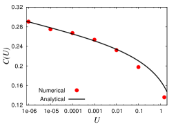
Figure 3: (color online) Dependence of $C(U)$ on $U$. Critical doping $\delta_{c}$ for transition from AF to FM state is given by $\delta_{c}=C(U)\frac{a}{W}$ (see eqn. (18)).

Upon doping the system with holes ($\delta>0$) or electrons $(\delta<0)$, the edge magnetization changes. For the AF configuration, we find

$$M^{AF}(\delta)=M^{AF}_{0}-\frac{|\delta|}{2}$$ (15)

while, interestingly, for the FM configuration

$$M^{FM}(\delta)\approx M^{FM}_{0}-s(U)\frac{W}{a}\delta^{2}$$ (16)

where $s(U)\approx\frac{\pi}{4}\left(1+\frac{2}{\ln(U/6)}\right)$. This leads to an energy difference between the two states

$$\Delta E(\delta)=-\frac{2Ue_{0}}{3}\left(\Delta M_{0}-\frac{|\delta|}{2}+s(U)\frac{W}{a}\delta^{2}\right)$$ (17)

to order $a/W$. We see that a first order transition from the AF to the FM configuration occurs at a critical doping

$$\delta_{c}=C(U)\frac{a}{W},\;\;C(U)=\mbox{$\frac{1-\sqrt{1-\ln 3\left(1+\frac{2}{\ln(U/6)}\right)}}{\pi\left(1+\frac{2}{\ln(U/6)}\right)}$}$$ (18)

Fig. 3 shows a comparison of this analytical result eqn. (18) with the numerical values of $C(U)$, and again, excellent quantitative agreement is found over many decades of $U$. For larger values of $U$ (such as that found in graphene), we find quantitative agreement up to about 10%. This owes to the fact that larger values of $U$ results in a small contribution from the bulk states, which is not captured in our edge mode based analytical theory. To the best of our knowledge, this is the first analytical and quantitative theory of the magnetism in zigzag-edged ribbons. An important point brought about by the theory is that interpreting the magnetism in these systems via a Stoner-Landau theory of the form eqn. (1) may be too simplistic. Indeed, the energy functional has a non-analytic structure $E(M)=AM^{2}+BM\ln DM$ ($A,B,D$ constants), that has roots in the sensory organ like Weber-Fechner response of zigzag-edge ribbons.

It is important to ensure that quantum fluctuations does not change the qualitative physics uncovered by the analytical theory. To this end, we performed variational Monte Carlo calculations of the ground state. Our trial wave function $|\varPsi\rangle=g^{D}|FS,M\rangle$, where $D$ is the double occupancy operator, $g$ is a the Gutzwiller factor that penalises double occupancy, $|FS,M\rangle$ is the filled Fermi sea state constructed by imposing an edge magnetization $M$ on the edge layers. For the AF configuration $M$ has opposite site on the two edges while for the FM configuration $M$ is equal on both edges. The optimal values of $g$ and $M$ are obtained so as to minimize the ground state energy. We have studied ribbons with $W\approx 6a$ with $U=1.5$. We find that the ground state at zero doping is the AF configuration, with an edge moment 0.20 which is expectedly smaller than the mean field value 0.27 owing to quantum fluctuations. Furthermore, the ground state changes to FM configuration at a critical doping $\delta$ of $0.025$. Both the AF and FM edge moments are stable, in that they remain unchanged upon increasing the length of the ribbon (for a given width $W$), proving that the magnetism is robust. While these calculations are prohibitively expensive for the determination the full phase diagram, these results provide evidence for the correctness of our analytical theory.

    

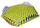
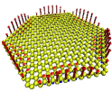
(a)                                  (b)

Figure 4: (color online) (a) Mean-field AF configuration in a zigzag edge terminated hexgonal nanodot $(U=1.5)$ (b) FM configuration obtained upon doping ($\delta=0.1$).

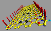
Figure 5: (color online) FM structure of the boron substituted zigzag edge terminated graphene nanoribbon obtained from first principles calculations. Dark atoms are borons and light ones are carbon. Hydrogen passivation of the edge atoms is also shown.

We have further investigated other zig-zag edge terminated nanostructures. For a undoped hexagonal nanodot, we find that the magnetic configuration has an AF structureFernandez-Rossier and Palacios (2007) as shown in Fig. 4(a), which upon doping, changes to a FM type (see Fig. 4(b)). Doping in practical applications can be achieved by gating. We have also explored possible chemical modification of graphene nanoribbons to produce an “internal doping” to engender the magnetic transition. Fig. 5 shows a FM structure of a zigzag edge terminated nanoribbon with boron atoms substitutedPanchakarla et al. (2009) in place of carbons, while the undoped nanoribbon has a AF configuration within the same calculation. As is evident, the results of this paper suggest many interesting possibilities of using zigzag edge terminated graphene nanostructures in applications.

AM thanks CPDF, IISc for support. VBS is grateful to DST for Ramanunjan and MONAMI grants, and DAE-SRC for generous support. The authors thank Umesh Waghmare for help with the first principles calculations, R. Shankar and Jayantha Vyasanakere for discussions.

References

- Westervelt (2008) R. M. Westervelt, Science 320, 324 (2008).
- Neto et al. (2009) A. H. C. Neto, F. Guinea, N. M. R. Peres, K. S. Novoselov, and A. K. Geim, Rev. Mod. Phys. 81, 109 (2009).
- Pati et al. (2011) S. K. Pati, T. Enoki, and C. N. R. Rao, eds., Graphene and its fascinating attributes (World Scientific, 2011).
- Bunch et al. (2005) J. Bunch, Y. Yaish, M. Brink, K. Bolotin, and P. McEuen, Nano Lett. 5, 287 (2005).
- Miao et al. (2007) F. Miao, S. Wijeratne, Y. Zhang, U. C. Coskun, W. Bao, and C. N. Lau, Science 317, 1530 (2007).
- Ponomarenko et al. (2008) L. A. Ponomarenko, F. Schedin, M. I. Katsnelson, R. Yang, E. W. Hill, K. S. Novoselov, and A. K. Geim, Science 320, 356 (2008).
- Wurm et al. (2009) J. Wurm, M. Wimmer, I. Adagideli, K. Richter, and H. U. Baranger, New Journal of Physics 11, 095022 (2009).
- Kotov et al. (2010) V. N. Kotov, B. Uchoa, V. M. Pereira, F. Guinea, and A. H. Castro Neto, ArXiv e-prints (2010), arXiv:1012.3484 [cond-mat.str-el] .
- Meng et al. (2010) Z. Y. Meng, T. C. Lang, S. Wessel, F. F. Assaad, and A. Muramatsu, Nature 464, 847 (2010).
- Pathak et al. (2010) S. Pathak, V. B. Shenoy, and G. Baskaran, Phys. Rev. B 81, 085431 (2010).
- Son et al. (2006a) Y. W. Son, M. L. Cohen, and S. G. Louie, Phys. Rev. Lett. 97, 216803 (2006a).
- Son et al. (2006b) Y. W. Son, M. L. Cohen, and S. G. Louie, Nature (London) 444, 347 (2006b).
- Peres et al. (2004) N. M. R. Peres, M. A. N. Araújo, and D. Bozi, Phys. Rev. B 70, 195122 (2004).
- Fernandez-Rossier and Palacios (2007) J. Fernandez-Rossier and J. J. Palacios, Phys. Rev. Lett. 99, 177204 (2007).
- Bhowmick and Shenoy (2008) S. Bhowmick and V. B. Shenoy, The Journal of Chemical Physics 128, 244717 (2008).
- Yazyev (2008) O. V. Yazyev, Phys. Rev. Lett. 101, 037203 (2008).
- Jung and MacDonald (2009) J. Jung and A. H. MacDonald, Phys. Rev. B 79, 235433 (2009).
- Ma et al. (2010) T. Ma, F. Hu, Z. Huang, and H.-Q. Lin, Applied Physics Letters 97, 112504 (2010).
- Yazyev (2010) O. V. Yazyev, Reports on Progress in Physics 73, 056501 (2010).
- Zhang et al. (2007) Y. Zhang, S. Talapatra, S. Kar, R. Vajtai, S. K. Nayak, and P. M. Ajayan, Phys. Rev. Lett. 99, 107201 (2007).
- Yazyev and Helm (2007) O. V. Yazyev and L. Helm, Phys. Rev. B 75, 125408 (2007).
- Ezawa (2007) M. Ezawa, Phys. Rev. B 76, 245415 (2007).
- Ramakrishna Matte et al. (2009) H. S. S. Ramakrishna Matte, K. S. Subrahmanyam, and C. N. R. Rao, ArXiv e-prints (2009), arXiv:0904.2739 [physics.chem-ph] .
- Rao et al. (2012) C. N. R. Rao, H. S. S. R. Matte, K. S. Subrahmanyam, and U. Maitra, Chem. Sci. 3, 45 (2012).
- Joly et al. (2010) V. L. J. Joly, M. Kiguchi, S.-J. Hao, K. Takai, T. Enoki, R. Sumii, K. Amemiya, H. Muramatsu, T. Hayashi, Y. A. Kim, M. Endo, J. Campos-Delgado, F. López-Urías, A. Botello-Méndez, H. Terrones, M. Terrones, and M. S. Dresselhaus, Phys. Rev. B 81, 245428 (2010).
- Kunstmann et al. (2011) J. Kunstmann, C. Özdoğan, A. Quandt, and H. Fehske, Phys. Rev. B 83, 045414 (2011).
- Nakada et al. (1996) K. Nakada, M. Fujita, G. Dresselhaus, and M. S. Dresselhaus, Phys. Rev. B 54, 17954 (1996).
- Wakabayashi et al. (1999) K. Wakabayashi, M. Fujita, H. Ajiki, and M. Sigrist, Phys. Rev. B 59, 8271 (1999).
- Brey and Fertig (2006a) L. Brey and H. A. Fertig, Phys. Rev. B 73, 195408 (2006a).
- Brey and Fertig (2006b) L. Brey and H. A. Fertig, Phys. Rev. B 73, 235411 (2006b).
- Zarea and Sandler (2009) M. Zarea and N. Sandler, Phys. Rev. B 79, 165442 (2009).
- Ryu and Hatsugai (2002) S. Ryu and Y. Hatsugai, Phys. Rev. Lett. 89, 077002 (2002).
- Kobayashi et al. (2005) Y. Kobayashi, K. Fukui, T. Enoki, K. Kusakabe, and Y. Kaburagi, Phys. Rev. B 71, 193406 (2005).
- Niimi et al. (2006) Y. Niimi, T. Matsui, H. Kambara, K. Tagami, M. Tsukada, and H. Fukuyama, Phys. Rev. B 73, 085421 (2006).
- Altland and Simons (2006) A. Altland and B. Simons, Condensed Matter Field Theory (Cambridge University Press, 2006).
- Yosida (1996) K. Yosida, Theory of Magnetism (Springer-Verlag, 1996).
- Bhowmick and Shenoy (2010) S. Bhowmick and V. B. Shenoy, Phys. Rev. B 82, 155448 (2010).
- Note (1) See http://en.wikipedia.org/wiki/Weber-Fechner_law.
- I. Bloch et al. (2012) I. Bloch, J. Dalibard, and S. Nascimbene, Nat. Phys. 8, 267 (2012).
- Tarruell et al. (2012) L. Tarruell, D. Greif, T. Uehlinger, G. Jotzu, and T. Esslinger, Nature 483, 302 (2012).
- Herbut (2006) I. F. Herbut, Phys. Rev. Lett. 97, 146401 (2006).
- Note (2) The slope in the inset of Fig. 2 is the coefficient of the linear term obtained by fitting a polynomial .
- Note (3) These calculations were done using Quantum Espresso code,Giannozzi et al. (2009) using plane-wave basis set and ultrasoft pseudo-potential. The energy cutoff for the plane-wave basis for wavefunctions is set to be 40 Ry. Electron exchange-correlation is treated with a local density approximation(LDA, Perdew-Zunger functional). Nanoribbons are simulated using a supercell geometry, with a vacuum layer of 15Å between any two periodic images of the ribbon. A k-point grid of 24x1x1 k points (periodic direction of the ribbon along x-axis) is used for sampling Brillouin zone integrations for this geometry.
- Panchakarla et al. (2009) L. S. Panchakarla, K. S. Subrahmanyam, S. K. Saha, A. Govindaraj, H. R. Krishnamurthy, U. V. Waghmare, and C. N. R. Rao, Advanced Materials 21, 4726 (2009).
- Giannozzi et al. (2009) P. Giannozzi, S. Baroni, N. Bonini, M. Calandra, R. Car, C. Cavazzoni, D. Ceresoli, G. L. Chiarotti, M. Cococcioni, I. Dabo, A. Dal Corso, S. de Gironcoli, S. Fabris, G. Fratesi, R. Gebauer, U. Gerstmann, C. Gougoussis, A. Kokalj, M. Lazzeri, L. Martin-Samos, N. Marzari, F. Mauri, R. Mazzarello, S. Paolini, A. Pasquarello, L. Paulatto, C. Sbraccia, S. Scandolo, G. Sclauzero, A. P. Seitsonen, A. Smogunov, P. Umari, and R. M. Wentzcovitch, Journal of Physics: Condensed Matter 21, 395502 (19pp) (2009).