UCI-TR-2012-10

TUM-HEP 849/12

FLAVOUR(267104)-ERC-21

CETUP*-12/008

On predictions from spontaneously broken flavor symmetries

Mu–Chun Chen

Department of Physics and Astronomy, University of California,
  Irvine, California 92697–4575, USA

Maximilian Fallbacher, Michael Ratz, Christian Staudt

Physik Department T30, Technische Universität München,
  James–Franck–Straße, 85748 Garching, Germany

We discuss the predictive power of supersymmetric models with flavor symmetries, focusing on the lepton sector of the standard model. In particular, we comment on schemes in which, after certain ‘flavons’ acquire their vacuum expectation values (VEVs), the charged lepton Yukawa couplings and the neutrino mass matrix appear to have certain residual symmetries. In most analyses, only corrections to the holomorphic superpotential from higher–dimensional operators are considered (for instance, in order to generate a realistic $\theta_{13}$ mixing angle). In general, however, the flavon VEVs also modify the Kähler potential and, therefore, the model predictions. We show that these corrections to the naive results can be sizable. Furthermore, we present simple analytic formulae that allow us to understand the impact of these corrections on the predictions for the masses and mixing parameters.

1 Introduction

The observed patterns of fermion masses and mixing may originate from underlying flavor symmetries. Typically, such flavor symmetries are assumed to be spontaneously broken by the vacuum expectation values (VEVs) of certain ‘flavon’ fields. Given a large enough flavor symmetry, one may thus hope to obtain a scheme that allows us to derive testable predictions. This applies, in particular, to settings in which flavor is generated at a very high scale, which cannot be directly accessed at colliders.

In this work, we study supersymmetric extensions of the standard model, in which flavor is generated at a high scale. For concreteness, we will take the scale of the flavon VEVs and the cut–off of the theory to be around the unification scale, though our results do not depend on this choice. On the other hand, one can imagine models in which there is a large difference between these two scales or which are renormalizable. In such models, non–renormalizable corrections including the corrections from the Kähler potential discussed in this letter become unimportant.

In order to be specific, we focus on the lepton sector of the theory, although our analysis can also be applied to the quark sector. Generically, the relevant superpotential reads, at the leading order,

$$\mathscr{W}_{\mathrm{leading}}~{}=~{}\frac{1}{\Lambda}(\Phi_{e})_{gf}\,L^{g}\,R^{f}\,H_{d}+\frac{1}{\Lambda\,\Lambda_{\nu}}(\Phi_{\nu})_{gf}\,L^{g}\,H_{u}\,L^{f}\,H_{u}\;,$$ (1.1)

where $L^{g}$ and $R^{f}$ (with the flavor indices $1\leq f,g\leq 3$) denote the lepton doublets and singlets, respectively, $H_{u}$ and $H_{d}$ are the Higgs doublets of the supersymmetric standard model, whereas $\Phi_{e}$ and $\Phi_{\nu}$ are the appropriate flavons. The two scales involved are the cut–off scale of the theory $\Lambda$ and the see–saw scale $\Lambda_{\nu}$. Once $\Phi_{e}$ and $\Phi_{\nu}$ acquire their VEVs, this leads to the effective superpotential

$$\mathscr{W}_{\mathrm{eff}}~{}=~{}(Y_{e})_{gf}\,L^{g}\,R^{f}\,H_{d}+\frac{1}{4}\kappa_{gf}\,L^{g}\,H_{u}\,L^{f}\,H_{u}\;.$$ (1.2)

In many models, one is left with a situation in which the flavon VEVs $\langle\Phi_{e}\rangle$ and $\langle\Phi_{\nu}\rangle$ respect certain residual symmetries, which are then dubbed symmetries of the charged lepton Yukawa couplings or the neutrino mass matrix, respectively (cf. figure 1). Predictions of such models are then based on these symmetries.

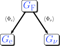
Figure 1: The flavor symmetry $G_{\mathrm{F}}$ gets broken to different subgroups in different sectors of the theory.

However, one may question if these are really robust predictions of the respective models. In particular, while certain terms in the superpotential appear to possess the aforementioned symmetries, the Lagrangean density often exhibits no residual symmetry. In other words, the combined VEVs $\langle\Phi_{e}\rangle$ and $\langle\Phi_{\nu}\rangle$ break the flavor symmetry completely. Moreover, the so–called predictions are subject to quantum corrections. For instance, the bi–maximal [1, 2] or tri–bi–maximal [3] mixing patterns are known not to be invariant under the renormalization group. On the other hand, the statements below (1.2) do not single out a particular scale. Therefore, one may wonder how such corrections can be consistent with the statement that the charged lepton Yukawa couplings or the neutrino mass matrix exhibit certain symmetries.

At the first glance, one may think that the corrections are related to possible higher–order terms that have to be added to the leading order superpotential (1.1). However, it is rather straightforward to construct models in which such higher–order corrections are absent to all orders. We will discuss such examples in a future publication [4].

The true solution to this puzzle is that models of the above type do not predict exact relations such as (tri–)bi–maximal mixing due to the presence of the Kähler corrections induced by the flavon VEVs [5, 6], even if higher order holomorphic corrections are absent. The Kähler potential should contain all terms consistent with the flavor symmetry,

$$K~{}=~{}K_{\mathrm{canonical}}+\Delta K\;,$$ (1.3)

where the relevant canonical terms include (with the SM gauge multiplets being set to zero)

$$K_{\mathrm{canonical}}~{}\supset~{}\left(L^{f}\right)^{\dagger}\,\delta_{fg}\,L^{g}+\left(R^{f}\right)^{\dagger}\,\delta_{fg}\,R^{g}\;,$$ (1.4)

and $\Delta K$ contains contractions of $L^{f}$ and $R^{f}$ and their Hermitean conjugates with the flavons. First of all, each of these terms in $\Delta K$ introduces one new parameter, i.e. its respective Kähler coefficient. Furthermore, once the flavons attain their VEVs, the flavor symmetry is broken thus modifying the Kähler metric. This modification $\Delta K$ of the Kähler potential can be written as

$$\Delta K~{}=~{}\left(L^{f}\right)^{\dagger}\,(\Delta K_{L})_{fg}\,L^{g}+\left(R^{f}\right)^{\dagger}\,(\Delta K_{R})_{fg}\,R^{g}\;,$$ (1.5)

with Hermitean matrices $\Delta K_{L}$ and $\Delta K_{R}$ whose structures are determined by the flavor symmetries and the flavon VEVs.

The necessary field redefinitions to compensate for these additional terms and to retrieve a canonical Kähler potential affect the superpotential. In particular, the Majorana mass matrix of the neutrinos and the Yukawa coupling matrix of the charged leptons are altered. This leads to changes of the neutrino mixing parameters irrespective of the existence of higher–order terms in the superpotential.

The purpose of this letter is to provide an analytic discussion of these changes, using similar methods as for the renormalization group (RG) equations in [7, 8] and for the Kähler corrections in [9, 10]. We will argue that corrections from these changes can be sizable and, therefore, without a better understanding of the Kähler potential, predictions from spontaneously broken flavor symmetries are incomplete. We leave a more detailed analysis for a future publication [4].

In section 2 we will start out by describing a well–known model that aims to explain the lepton mixing only with terms coming from the superpotential. Section 3 is then devoted to the discussion of the Kähler corrections. Based on the results obtained in sections 3.1 and 3.2 and using analytic formulae presented in section 3.4, we will argue in section 3.5 that the changes compared to an analysis without Kähler corrections are substantial. Finally, section 4 summarizes our conclusions.

2 Predictions from the superpotential couplings

We first focus on the predictions of flavor models from the holomorphic couplings of the theory, i.e. the superpotential. To be specific, we base our discussion on an example model [11] with an $\mathrm{A}_{4}$ flavor symmetry [12], which serves as a prototype setting leading to tri–bi–maximal lepton mixing.

Since the following discussion heavily depends on the group structure of $\mathrm{A}_{4}$, we first review the necessary facts. In particular, these are the possible contractions of fields transforming under this symmetry. $\mathrm{A}_{4}$ has four inequivalent irreducible representations: three one–dimensional representations, denoted by $\boldsymbol{1}$, $\boldsymbol{1^{\prime}}$ and $\boldsymbol{1^{\prime\prime}}$, and one triplet, denoted by $\boldsymbol{3}$. The relevant multiplication law is

$$\boldsymbol{3}\otimes\boldsymbol{3}~{}=~{}\boldsymbol{1}\oplus\boldsymbol{1^{\prime}}\oplus\boldsymbol{1^{\prime\prime}}\oplus\boldsymbol{3}_{\mathrm{s}}\oplus\boldsymbol{3}_{\mathrm{a}}\;,$$ (2.1)

where $\boldsymbol{3}_{\mathrm{s}}$ and $\boldsymbol{3}_{\mathrm{a}}$ denote the symmetric and the antisymmetric triplet combinations, respectively. In terms of the components of the two triplets, $\boldsymbol{a}$ and $\boldsymbol{b}$,

$$\left(\boldsymbol{a}\otimes\boldsymbol{b}\right)_{\boldsymbol{1}} = a_{1}\,b_{1}+a_{2}\,b_{3}+a_{3}\,b_{2}\;,$$ (2.2a)

$$\left(\boldsymbol{a}\otimes\boldsymbol{b}\right)_{\boldsymbol{1^{\prime}}} = a_{3}\,b_{3}+a_{1}\,b_{2}+a_{2}\,b_{1}\;,$$ (2.2b)

$$\left(\boldsymbol{a}\otimes\boldsymbol{b}\right)_{\boldsymbol{1^{\prime\prime}}} = a_{2}\,b_{2}+a_{1}\,b_{3}+a_{3}\,b_{1}\;,$$ (2.2c)

$$\left(\boldsymbol{a}\otimes\boldsymbol{b}\right)_{\boldsymbol{3}_{\mathrm{s}}} = \frac{1}{\sqrt{2}}\,\left(\begin{array}[]{c}2a_{1}\,b_{1}-a_{2}\,b_{3}-a_{3}\,b_{2}\\ 2a_{3}\,b_{3}-a_{1}\,b_{2}-a_{2}\,b_{1}\\ 2a_{2}\,b_{2}-a_{1}\,b_{3}-a_{3}\,b_{1}\end{array}\right)\;,$$ (2.2g)

$$\left(\boldsymbol{a}\otimes\boldsymbol{b}\right)_{\boldsymbol{3}_{\mathrm{a}}} = \mathrm{i}\,\sqrt{\frac{3}{2}}\,\left(\begin{array}[]{c}a_{2}\,b_{3}-a_{3}\,b_{2}\\ a_{1}\,b_{2}-a_{2}\,b_{1}\\ a_{3}\,b_{1}-a_{1}\,b_{3}\end{array}\right)\;,$$ (2.2k)

where $\left(\boldsymbol{a}\otimes\boldsymbol{b}\right)_{\boldsymbol{R}}$ indicates that $\boldsymbol{a}$ and $\boldsymbol{b}$ are contracted to the representation $\boldsymbol{R}$. Note that there are different conventions for normalizing the triplets $\boldsymbol{3}_{i}$ in the literature, and the corresponding factors can be absorbed in the Kähler coefficients.

A well–known example for an $\mathrm{A}_{4}$ tri–bi–maximal model is given by Altarelli et al. [11]. In this model, under $\mathrm{A}_{4}$ the three generations of left–handed lepton doublets transform as a triplet, $L\sim$ $\boldsymbol{3}$, the right–handed charged leptons, $e_{\mathrm{R}}$, $\mu_{\mathrm{R}}$ and $\tau_{\mathrm{R}}$, transform as $\boldsymbol{1}$, $\boldsymbol{1^{\prime\prime}}$, and $\boldsymbol{1^{\prime}}$, respectively, and the Higgs fields $H_{u}$ and $H_{d}$ transform as pure singlets $\boldsymbol{1}$. Tri–bi–maximal mixing is achieved by the introduction of three flavons: $\Phi_{\nu}$ and $\Phi_{e}$, both of which transform as triplets under the $\mathrm{A}_{4}$ symmetry, and a pure $\mathrm{A}_{4}$ singlet $\xi\sim$ $\boldsymbol{1}$. The couplings of the flavons to the SM fields are (cf. equation (1.1))

$$\mathscr{W}_{\nu} = \frac{\lambda_{1}}{\Lambda\,\Lambda_{\mathrm{\nu}}}\,\left\{\left[(L\,H_{u})\otimes(L\,H_{u})\right]_{\boldsymbol{3}_{\mathrm{s}}}\otimes\Phi_{\nu}\right\}_{\boldsymbol{1}}+\frac{\lambda_{2}}{\Lambda\,\Lambda_{\mathrm{\nu}}}\,\left[(L\,H_{u})\otimes(L\,H_{u})\right]_{\boldsymbol{1}}\,\xi\;,$$ (2.3)

$$\mathscr{W}_{e} = \frac{h_{e}}{\Lambda}\,\left(\Phi_{e}\otimes L\right)_{\boldsymbol{1}}\,H_{d}\,e_{\mathrm{R}}+\frac{h_{\mu}}{\Lambda}\,\left(\Phi_{e}\otimes L\right)_{\boldsymbol{1^{\prime}}}\,H_{d}\,\mu_{\mathrm{R}}+\frac{h_{\tau}}{\Lambda}\,\left(\Phi_{e}\otimes L\right)_{\boldsymbol{1^{\prime\prime}}}\,H_{d}\,\tau_{\mathrm{R}}\;,$$ (2.4)

where, as before, $\Lambda$ and $\Lambda_{\nu}$ are the flavon scale and the see–saw scale, respectively.

Furthermore, the model is assumed to be invariant under a $\mathbbm{Z}_{4}$ symmetry under which $\Phi_{\nu}$ and $\xi$ change sign, whereas $\Phi_{e}$ is not charged under this symmetry. The transformation properties of the leptons under this $\mathbbm{Z}_{4}$ are given by $L\rightarrow\mathrm{i}L$ and $R\rightarrow-\mathrm{i}R$.

The $\mathrm{A}_{4}$ symmetry is then broken by assigning the following VEVs to the flavons.

$$\langle\Phi_{\nu}\rangle = \left(v,v,v\right)\;,$$ (2.5a)

$$\langle\Phi_{e}\rangle = \left(v^{\prime},0,0\right)\;,$$ (2.5b)

$$\langle\xi\rangle = w\;.$$ (2.5c)

The resulting charged lepton Yukawa matrix after electroweak symmetry breaking is diagonal and reads

$$m_{e}~{}=~{}v_{d}\,\operatorname{diag}\left(y_{e},\,y_{\mu},\,y_{\tau}\right)\;,$$ (2.6)

where $v_{d}$ is the VEV of $H_{d}$ and $y_{e,\,\mu,\,\tau}=h_{e,\,\mu,\,\tau}\,\frac{v^{\prime}}{\Lambda}$. The neutrino mass matrix, however, is non–diagonal. It is given by

$$m_{\nu}~{}=~{}\begin{pmatrix}a+2d&-d&-d\\ -d&2d&a-d\\ -d&a-d&2d\end{pmatrix}\;,$$ (2.7)

with $a=2\lambda_{2}\,\frac{v_{u}^{2}}{\Lambda_{\mathrm{\nu}}}\,\frac{w}{\Lambda}$ and $d=\sqrt{2}\lambda_{1}\,\frac{v_{u}^{2}}{\Lambda_{\nu}}\,\frac{v}{\Lambda}$, where $v_{u}$ is the VEV of $H_{u}$. The neutrino mass matrix is diagonalized by the tri–bi–maximal mixing matrix

$$U_{\mathrm{TBM}}~{}=~{}\begin{pmatrix}\sqrt{\frac{2}{3}}&\frac{1}{\sqrt{3}}&0\\ -\frac{1}{\sqrt{6}}&\frac{1}{\sqrt{3}}&-\frac{1}{\sqrt{2}}\\ -\frac{1}{\sqrt{6}}&\frac{1}{\sqrt{3}}&\frac{1}{\sqrt{2}}\end{pmatrix}\;.$$ (2.8)

Since the charged lepton Yukawa matrix is already diagonal, the mixing matrix $U_{\mathrm{PMNS}}$ is identical to $U_{\mathrm{TBM}}$ and the corresponding mixing angles are shown in table 2.1.

	$\theta_{12}$	$\theta_{13}$	$\theta_{23}$
TBM prediction:	$\arctan{\left(\sqrt{0.5}\right)}\approx 35.3^{\circ}$	$0$	$45^{\circ}$
Best fit values $(\pm 1\sigma)$:	$\left(33.6^{+1.1}_{-1.0}\right)^{\circ}$	$\left(8.93^{+0.46}_{-0.48}\right)^{\circ}$	$\left(38.4^{+1.4}_{-1.2}\right)^{\circ}$

Table 2.1: Tri–bi–maximal prediction for the neutrino mixing angles and best fit values from the global fit by [13].

In the same table, the best fit values from the global fit on neutrino mixing parameters by [13] are quoted. As one can see, the recent measurement of $\theta_{13}$ has revealed a huge deviation from the predicted TBM value. In addition, the TBM prediction for $\theta_{23}$ also does not agree well with the current global fit value, which indicates a sizable deviation from maximal mixing.

These deviations seem to be difficult to explain with corrections coming from the superpotential only. On the other hand, they might originate from the flavon VEV–induced Kähler corrections as we shall see in the following section.

3 Corrections due to Kähler potential terms

As discussed in the introduction, apart from the canonical terms, there may exist extra terms in the Kähler potential induced by the flavon VEVs. In the $\mathrm{A}_{4}$ example model discussed above, these terms are contractions of the left–handed lepton doublets, which transform as an $\mathrm{A}_{4}$ triplet, with one or several flavons. After the flavons acquire a VEV, these terms lead to a Kähler metric with off–diagonal terms. We shall sketch the computation for the $\mathrm{A}_{4}$ example model, leaving the general derivation to [4].

3.1 Linear flavon corrections

The leading order contributions are linear in the flavons. These linear terms are only suppressed by one power of the ratio of the flavon VEV to the fundamental scale of the theory. The contributions in the $\mathrm{A}_{4}$ model discussed above read schematically

$$\Delta K_{\mathrm{linear}}~{}=~{}\sum\limits_{i\,\in\{\mathrm{a},\mathrm{s}\}}\left(\frac{\kappa_{\Phi_{\nu}}^{(i)}}{\Lambda}\,\Delta K_{L^{\dagger}\,(L\otimes\Phi_{\nu})_{\boldsymbol{3}_{i}}}^{(i)}+\frac{\kappa_{\Phi_{e}}^{(i)}}{\Lambda}\,\Delta K_{L^{\dagger}\,(L\otimes\Phi_{e})_{\boldsymbol{3}_{i}}}^{(i)}\right)+\frac{\kappa_{\xi}}{\Lambda}\,\Delta K_{\xi L^{\dagger}L}+\text{h.c.}\;.$$ (3.1)

However, it is easy to forbid any of these terms, by introducing an additional symmetry (such as the $\mathbbm{Z}_{4}$ symmetry in the example model) under which all flavons are charged. Hence, we do not consider the linear flavon corrections any further but turn to contributions which are quadratic in the flavons, and cannot be forbidden by any (conventional) symmetry.

3.2 Second order corrections

The corrections to the Kähler metric which are second order in the flavon VEVs can be divided into two classes. The first class consists of terms that are of the form $(L\Phi_{\nu})^{\dagger}(L\Phi_{\nu})$ or $(L\Phi_{e})^{\dagger}(L\Phi_{e})$, i.e. they are quadratic in one specific flavon. As mentioned above, these cannot be forbidden by a (conventional) symmetry. This is not true for the second class which consists of terms of the form $(L\Phi_{\nu})^{\dagger}(L\Phi_{e})$, i.e. they are contractions involving two different flavons. For the same reasons as in the linear case, the second class is not considered here.

All corrections discussed here can thus be obtained from suitable contractions of the terms $(L\otimes\Phi_{\nu})_{\boldsymbol{R}}^{\dagger}(L\otimes\Phi_{\nu})_{\boldsymbol{R^{\prime}}}$ and $(L\otimes\Phi_{e})_{\boldsymbol{R}}^{\dagger}(L\otimes\Phi_{e})_{\boldsymbol{R^{\prime}}}$ using the rules stated in (2.2). Although there are numerous possible contractions, several of them give the same correction $\Delta K$ to the Kähler metric up to the respective Kähler coefficient which is a complex number. All in all, there are 5 different matrices which have to be considered. The first three matrices

$$P_{\mathrm{I}}~{}=~{}\operatorname{diag}(1,0,0)\;,\quad P_{\mathrm{II}}~{}=~{}\operatorname{diag}(0,1,0)\quad\text{and}\quad P_{\mathrm{III}}~{}=~{}\operatorname{diag}(0,0,1)$$ (3.2a)

come from contractions of $$L \Phi_{e} (v^{\prime})^{2} v^{\prime} \Phi_{e} \langle\Phi_{e}\rangle=(v^{\prime},0,0)$$ with . That is, their contribution is proportional to , where is the size of the VEV of , . The remaining two matrices,

$$P_{\mathrm{IV}}~{}=~{}\begin{pmatrix}1&1&1\\ 1&1&1\\ 1&1&1\end{pmatrix}\quad\text{and}\quad P_{\mathrm{V}}~{}=~{}\begin{pmatrix}0&\mathrm{i}&-\mathrm{i}\\ -\mathrm{i}&0&\mathrm{i}\\ \mathrm{i}&-\mathrm{i}&0\end{pmatrix}\;,$$ (3.2b)

are contributions due to $\Phi_{\nu}$. Therefore, their contribution in the Kähler potential is proportional to $v^{2}$ which is defined by $\langle\Phi_{\nu}\rangle=(v,v,v)$.

The third flavon $\xi$ does not yield any relevant contribution since it can only give an overall normalization factor, which does not change the mixing angles. Another way of understanding this is by observing that $\xi$ is not a flavon in the strict sense as it transforms trivially under $\mathrm{A}_{4}$, such that its VEV does not break $\mathrm{A}_{4}$.

Each of the corrections is suppressed by the cut–off scale $\Lambda$ to the second power. Furthermore, each of the terms comes with its own Kähler coefficient $\kappa_{i}$, which, in general, is complex. Adding the Hermitean conjugate always cancels either the term with the real or the imaginary part of $\kappa_{i}$. We arranged our matrices $P_{i}$ in a way that all the coefficients can be chosen real. However, the values of the Kähler coefficients $\kappa_{i}$ are not fixed by the symmetries of the model and, therefore, their presence introduces additional continuous parameters. One may hope to be able to compute them in a possible UV completion of the model. Generically, these higher order terms in the Kähler potential can come from integrating out heavy modes that are required to complete the model in the UV. Since one expects to have several of such modes, whose couplings to the zero modes of the theory can moreover be unsuppressed, and due to group theoretical factors, the Kähler coefficients can be of the order unity or even larger.

Let us comment that the Kähler corrections will, in general, also be important for the question of VEV alignment. That is, the scalar potential that fixes the VEVs of the flavons at some desired pattern will also be subject to these corrections, and one might expect deviations from the fully symmetric structures (such as those specified in (2.5)). We plan to discuss these issues in more detail in our follow–up paper [4].

3.3 Corrections from the right–handed leptons

In principle, there are also contributions from the right–handed sector. However, in the model discussed here, all right–handed charged leptons are $\mathrm{A}_{4}$ singlets, and therefore, the corresponding Kähler corrections can be made diagonal. More precisely, possible off–diagonal terms can easily be forbidden by additional symmetries (cf. the discussion in 3.1). Since our basis is chosen such that the original charged lepton Yukawa matrix is diagonal, a diagonal redefinition of the right–handed leptons $R^{f}$ cannot induce any off–diagonal terms in the Yukawa matrix. Hence, the transformed Yukawa matrix is still diagonal, only the eigenvalues may be changed. This implies that such a field redefinition does not have any influence on the neutrino mixing matrix. In conclusion, the model can be modified such that the corrections from the right–handed sector cannot change the mixing parameters, and therefore, they are not discussed any further.

3.4 Analytic formulae for Kähler corrections

It is possible to derive some simple analytic formulae for the change of the mixing parameters due to small non–diagonal terms in the Kähler potential. Suppose that, after the flavon fields attain their VEVs, the Kähler potential reads

$$K~{}=~{}K_{\mathrm{canonical}}+\Delta K~{}=~{}L^{\dagger}\,(1-2x\,P)\,L$$ (3.3)

with a Hermitean matrix $P$ and an infinitesimal expansion parameter $x$. The Kähler metric is diagonalized to first order in $x$ by the field redefinition

$$L~{}\rightarrow~{}L^{\prime}~{}=~{}(1-x\,P)\,L\;.$$ (3.4)

This field redefinition affects the effective neutrino mass operator $\kappa$ for the canonically normalized left–handed doublets $L^{\prime\,f}$,

$$\mathscr{W}_{\nu}~{}\simeq~{}\frac{1}{4}\,(L^{\prime\,f}H_{u})^{T}\,\left[\kappa+x\,P^{T}\,\kappa+x\,\kappa\,P\right]_{gf}\,L^{\prime\,g}H_{u}\;,$$ (3.5)

where $\kappa\cdot v_{u}^{2}=2m_{\nu}$ with $m_{\nu}$ specified in equation (2.7). That is, the neutrino mass operator has effectively become $x$–dependent, and the resulting neutrino mass matrix depends on $x$ as

$$m_{\nu}(x)~{}\simeq~{}m_{\nu}+x\,P^{T}\,m_{\nu}+x\,m_{\nu}\,P\;.$$ (3.6)

This leads to the differential equation

$$\frac{\mathrm{d}m_{\nu}}{\mathrm{d}x}~{}=~{}P^{T}\,m_{\nu}+m_{\nu}\,P$$ (3.7)

for the neutrino mass matrix, which holds locally at $x=0$. This equation has the same structure as the one governing the RG evolution of the mass operator. In [7], analytic formulae describing the evolution of the mixing parameters have been derived. Using an analogous procedure, one can compute the derivatives of the mixing parameters at $x=0$.

To this end, one derives a differential equation for $U_{\nu}$ from equation (3.7) by substituting $U_{\nu}^{*}D_{\nu}U_{\nu}^{\dagger}$ for $m_{\nu}$, where $D_{\nu}$ is the diagonalized neutrino mass matrix. This equation can then be used to determine the entries of $U_{\nu}^{\dagger}\,\mathrm{d}U_{\nu}/\mathrm{d}x$, which can also be written in terms of the mixing angles and phases of the standard parametrization of $U_{\mathrm{PMNS}}$. A similar procedure was also already used in [10] to compute Kähler corrections.

With the Kähler coefficients and the ratios of flavon VEVs and high scale $\Lambda$ as input parameters, the resulting formulae can be used to predict the change of the mixing parameters due to a non–trivial Kähler metric for not too large deviations from the canonical one. The detailed derivation of these formulae and a more thorough discussion of their implications are deferred to a later publication [4]. Here, we only discuss some examples for the case of the $\mathrm{A}_{4}$ model described above.

Let us briefly comment on the relation of Kähler corrections and RG evolution (cf. also [9]). First of all, unlike RG corrections, the Kähler corrections are not loop–suppressed. Furthermore, while they are similar in structure, generally the Kähler corrections can be along different directions. In particular, they are not restricted to the diagonal. For example, in the model considered, the main RG correction is essentially along the direction specified by the matrix $P_{\mathrm{III}}$ in equation (3.2a). The Kähler corrections, however, can be along any of the five directions in equation (3.2). Which one(s) of these five directions dominate(s) depends upon the UV completion of the model.

3.5 Implications for the $\boldsymbol{\mathrm{A}_{4}}$ example model

With the analytic formulae whose derivation was sketched briefly in the foregoing section, we can compute the Kähler corrections which arise in the example model [11] discussed in section 2.

The most interesting correction is due to the matrix $P_{\mathrm{V}}$ in equation (3.2). It originates from the term $(L\otimes\Phi_{\nu})_{\boldsymbol{3}_{\mathrm{a}}}^{\dagger}\,(L\otimes\Phi_{\nu})_{\boldsymbol{3}_{\mathrm{s}}}+\text{h.c.}$ in the Kähler potential. Performing the $\mathrm{A}_{4}$ contractions carefully, one finds that the additional Kähler potential term is given by

$$\Delta K~{}=~{}\kappa_{\mathrm{V}}\cdot\frac{v^{2}}{\Lambda^{2}}\cdot 3\sqrt{3}\cdot(L^{f})^{\dagger}\,(P_{\mathrm{V}})_{fg}\,(L^{g})\;,$$ (3.8)

where $\kappa_{\mathrm{V}}$ denotes the relevant Kähler coefficient.

The analytic formula for the change of $\theta_{13}$ compared to the case of a canonical Kähler potential reads

$$\Delta\theta_{13} = \kappa_{\mathrm{V}}\cdot\frac{v^{2}}{\Lambda^{2}}\cdot 3\sqrt{3}\cdot\frac{1}{\sqrt{2}}\left(\frac{2m_{1}}{m_{1}+m_{3}}+\frac{m_{e}^{2}}{m_{\mu}^{2}-m_{e}^{2}}+\frac{m_{e}^{2}}{m_{\tau}^{2}-m_{e}^{2}}\right)$$ (3.9)

$$\simeq \kappa_{\mathrm{V}}\cdot\frac{v^{2}}{\Lambda^{2}}\cdot 3\sqrt{6}~{}\frac{m_{1}}{m_{1}+m_{3}}\;,$$

where the $m_{i}$ are the neutrino masses. In the second line, the very small contribution of the charged leptons has been neglected.

In the following, we assume that the normal neutrino hierarchy is realised and use the current PDG [14] values for the differences of the mass–squares,

$$\Delta m_{21}^{2}~{}=~{}7.50\cdot 10^{-5}\,(\text{e\kern-0.59998ptV})^{2}\quad\text{and}\quad\Delta m_{32}^{2}~{}=~{}2.32\cdot 10^{-3}\,(\text{e\kern-0.59998ptV})^{2}\;,$$ (3.10)

as input parameters. Moreover, the ratio of VEV to the fundamental scale $v/\Lambda$ is set to $0.2$ and the Kähler coefficient $\kappa_{\mathrm{V}}$ is set to 1. Then the variation of the change of $\theta_{13}$ with $m_{1}$ can be studied and is shown in figure 2.

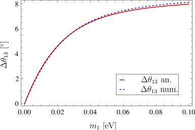
Figure 2: Change of $\theta_{13}$ due to the Kähler correction $\Delta K$ shown in equation (3.8) for $\kappa_{\mathrm{V}}\,v^{2}/\Lambda^{2}=(0.2)^{2}$. The continuous line shows the result of equation (3.9), which was obtained using a linear approximation (cf. section 3.4), while the dashed line shows the result of a numerical computation. As one can see, the linear approximation yields a very accurate estimate on the true change $\Delta\theta_{13}$.

The deviation from the exact tri–bi–maximal prediction is substantial, especially in the regime where $m_{1}$ gets large. This is also easy to see from the analytic formula that asymptotically approaches a value of $\Delta\theta_{13}\approx 8.42^{\circ}$ for $m_{1}\rightarrow\infty$. Based on the fact that the differential equation for the Kähler corrections is similar in structure to the RG equation, our numerical result is consistent with the expectation, as $m_{1}\rightarrow\mathcal{O}(0.1\>\text{e\kern-0.59998ptV})$ corresponds to the near degenerate regime for the neutrino masses, where an enhanced correction to the mixing angle is expected.

In contrast to the case of $\theta_{13}$, the changes of $\theta_{12}$ and $\theta_{23}$ are predicted to be zero if one uses the linear extrapolation of their changes starting from the tri–bi–maximal mixing pattern. However, as we have seen above, $\theta_{13}$ can undergo a substantial change such that also the other two mixing angles change due to higher order non-linear terms. We have confirmed this behavior numerically, using the MixingParameterTools package [8]. The dependence of the change on the lightest neutrino mass $m_{1}$ is shown in figure 3. Both changes are significantly smaller than the one of $\theta_{13}$.

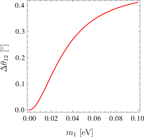
(a) $\Delta\theta_{12}$.

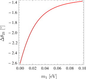
(b) $\Delta\theta_{23}$.

Figure 3: Changes of (a) $\theta_{12}$ and (b) $\theta_{23}$ due to the Kähler correction $\Delta K$ shown in equation (3.8) for $\kappa_{\mathrm{V}}\,v^{2}/\Lambda^{2}=(0.2)^{2}$ computed numerically.

A further interesting consequence of the Kähler correction is the generation of CP violation. It arises due to the fact that the matrix $P_{\mathrm{V}}$ is complex. In fact, the Dirac CP phase $\delta$, which is not properly defined for exact tri–bi–maximal mixing due to $\theta_{13}=0$, is close to $\delta=3\pi/2$ taking into account the corrections. Note that similar relations can also be obtained from the holomorphic superpotential in models with $T^{\prime}$ flavor symmetry [15].

There can, of course, be additional contributions from other $P$ matrices. Hence, as a second example of the implications of the Kähler corrections, we discuss the case of $P_{\mathrm{IV}}$, which arises in all possible singlet contractions of $\Phi_{\nu}$, e.g. $(L\otimes\Phi_{\nu})_{\boldsymbol{1}}^{\dagger}\,(L\otimes\Phi_{\nu})_{\boldsymbol{1}}+\text{h.c}$. Including all coefficients, the corresponding term in the Kähler potential is given by

$$\Delta K~{}=~{}\kappa_{\mathrm{IV}}\cdot\frac{v^{2}}{\Lambda^{2}}\cdot 2\cdot(L^{f})^{\dagger}\,(P_{\mathrm{IV}})_{fg}\,(L^{g})\;.$$ (3.11)

The resulting analytic formulae for the mixing angles are, in agreement with the numerical computation, independent of the neutrino masses; they only depend on the charged lepton masses, e.g.

$$\Delta\theta_{12}~{}=~{}\kappa_{\mathrm{IV}}\cdot\frac{v^{2}}{\Lambda^{2}}\cdot\sqrt{2}\cdot\frac{\left(m_{\mu}^{2}\,m_{\tau}^{2}-m_{e}^{4}\right)}{\left(m_{e}^{2}-m_{\mu}^{2}\right)\left(m_{e}^{2}-m_{\tau}^{2}\right)}\;.$$ (3.12)

$P_{\mathrm{IV}}$ does not induce any change of $\theta_{13}$, but the other two mixing angles are shifted. In fact, the resulting change of $\theta_{12}$ for $\kappa_{\mathrm{IV}}\,v^{2}/\Lambda^{2}=(0.2)^{2}$ is about $3.2^{\circ}$ while the the change of $\theta_{23}$ is $-2.3^{\circ}$. In particular, for both sign choices of $\kappa_{\mathrm{IV}}$ one of the two mixing angles is driven further away from its best fit value.

The chosen examples illustrate that predictions which are solely based on the inspection of the superpotential are not very reliable. Indeed, for example, the global fit value for $\theta_{13}=\left(8.93^{+0.46}_{-0.48}\right)^{\circ}$ [13] (cf. table 2.1) can be accommodated without resorting to higher–order contributions from the superpotential, provided the neutrino mass spectrum is not too hierarchical, the ratio of flavon VEV to the fundamental scale $v/\Lambda$ is of the order of the Cabibbo angle and the Kähler coefficient $\kappa_{\mathrm{V}}$ is of order one. On the other hand, there are Kähler corrections that drive the theoretical predictions for the mixing parameters far away from their current best fit values. Without any organizing principle for the Kähler potential, it seems to be hardly possible to derive definite predictions from discrete flavour symmetries. Our results also show that the Kähler corrections can be more significant than the effects of the RG evolution.

4 Conclusions

We have carefully re–examined models in which different flavons appear to break a given flavor symmetry $G_{\mathrm{F}}$ down to different subgroups in different sectors of the theory. In the context of supersymmetric settings, the fact that there is no residual symmetry in the full Lagrangean manifests itself in corrections to the Kähler potential $K$ that break $G_{\mathrm{F}}$ in all subsectors. We have argued that the corresponding higher–order terms in $K$ are, in a way, unavoidable as they cannot be forbidden by any (conventional) symmetry. These terms come with certain coefficients, which are not determined by the symmetries of the model and, therefore, introduce additional continuous parameters. We have also argued that the Kähler corrections are generically much larger and, therefore, more relevant than renormalization effects, which can also be understood as Kähler corrections along a very specific direction.

In order to make our analysis more concrete, we have outlined the discussion of the corrections in a model based on the flavor symmetry $G_{\mathrm{F}}=\mathrm{A}_{4}\times\mathbbm{Z}_{4}$ [11]. We have presented results of an analytic discussion of the Kähler corrections, i.e. simple analytic formulae that allow us to express the change in the prediction on the mixing parameters induced by the respective flavon VEVs. While leaving the full discussion for a future publication [4], we have explicitly shown that in the simple $\mathrm{A}_{4}$ model, which predicts tri–bi–maximal mixing at leading order, one of the flavon VEVs induces a large variation of the mixing angle $\theta_{13}$ while leaving the other mixing angles essentially unchanged. An optimistic interpretation of this possibility may amount to the statement that even simple models like the one discussed here can be consistent with the recent measurement of $\theta_{13}$ [16, 17, 18]. One the other hand, one may be more critical and question the actual predictive power of a large class of flavor models that exist in the literature. As we have seen in our second example, Kähler corrections might significantly modify the predictions of a model. Hence, one may actually argue that even in very simple models, a better understanding of the Kähler potential is mandatory in order to achieve an accuracy that can compete with the contemporary experimental precision.

In a future publication [4], we will provide more details on the derivation of the analytic formulae used in this letter.

Acknowledgments

M.-C.C. would like to thank TU München, where part of the work was done, for hospitality. M.R. would like to thank the UC Irvine, where part of this work was done, for hospitality. This work was partially supported by the Deutsche Forschungsgemeinschaft (DFG) through the cluster of excellence “Origin and Structure of the Universe” and the Graduiertenkolleg “Particle Physics at the Energy Frontier of New Phenomena”. This research was done in the context of the ERC Advanced Grant project “FLAVOUR” (267104), and was partially supported by the U.S. National Science Foundation under Grant No. PHY-0970173. We thank the Aspen Center for Physics, where this discussion was initiated, the Galileo Galilei Institute for Theoretical Physics (GGI), the Simons Center for Geometry and Physics in Stony Brook, and the Center for Theoretical Underground Physics and Related Areas (CETUP* 2012) in South Dakota for their hospitality and for partial support during the completion of this work.

References

- [1] F. Vissani, arXiv:hep-ph/9708483 [hep-ph].
- [2] V. D. Barger, S. Pakvasa, T. J. Weiler, and K. Whisnant, Phys.Lett. B437 (1998), 107, arXiv:hep-ph/9806387 [hep-ph].
- [3] P. Harrison, D. Perkins, and W. Scott, Phys.Lett. B530 (2002), 167, arXiv:hep-ph/0202074 [hep-ph].
- [4] M.-C. Chen, M. Fallbacher, Y. Omura, M. Ratz, and C. Staudt, in preparation.
- [5] M. Leurer, Y. Nir, and N. Seiberg, Nucl. Phys. B420 (1994), 468, hep-ph/9310320.
- [6] E. Dudas, S. Pokorski, and C. A. Savoy, Phys.Lett. B356 (1995), 45, arXiv:hep-ph/9504292 [hep-ph].
- [7] S. Antusch, J. Kersten, M. Lindner, and M. Ratz, Nucl.Phys. B674 (2003), 401, arXiv:hep-ph/0305273 [hep-ph].
- [8] S. Antusch, J. Kersten, M. Lindner, M. Ratz, and M. A. Schmidt, JHEP 03 (2005), 024, hep-ph/0501272.
- [9] S. Antusch, S. F. King, and M. Malinsky, Phys.Lett. B671 (2009), 263, arXiv:0711.4727 [hep-ph].
- [10] S. Antusch, S. F. King, and M. Malinsky, JHEP 0805 (2008), 066, arXiv:0712.3759 [hep-ph].
- [11] G. Altarelli and F. Feruglio, Nucl.Phys. B741 (2006), 215, arXiv:hep-ph/0512103 [hep-ph].
- [12] E. Ma, Phys.Rev. D70 (2004), 031901, arXiv:hep-ph/0404199 [hep-ph].
- [13] G. Fogli, E. Lisi, A. Marrone, D. Montanino, A. Palazzo, et al., Phys.Rev. D86 (2012), 013012, arXiv:1205.5254 [hep-ph].
- [14] Particle Data Group, J. Beringer et al., Phys.Rev. D86 (2012), 010001.
- [15] M.-C. Chen and K. Mahanthappa, Phys.Lett. B681 (2009), 444, arXiv:0904.1721 [hep-ph].
- [16] DOUBLE-CHOOZ Collaboration, Y. Abe et al., Phys.Rev.Lett. 108 (2012), 131801, arXiv:1112.6353 [hep-ex].
- [17] DAYA-BAY Collaboration, F. An et al., Phys.Rev.Lett. 108 (2012), 171803, arXiv:1203.1669 [hep-ex].
- [18] RENO collaboration, J. Ahn et al., Phys.Rev.Lett. 108 (2012), 191802, arXiv:1204.0626 [hep-ex].