Distribution Of Wealth In A Network Model Of The Economy

Abstract

We show, analytically and numerically, that wealth distribution in the Bouchaud-Mézard network model of the economy is described by a three-parameter generalized inverse gamma distribution. In the mean-field limit of a network with any two agents linked, it reduces to the inverse gamma distribution.

I Introduction

Wealth distribution has become a subject of keen interest in econophysics research.yakovenko2009 Here, we study a network model of the economy proposed by Bouchaud and Mézard (BM).bouchaud2000 In the mean field (MF) limit of a completely connected network, where any two agents in the network are linked, the model yields the inverse gamma (IGa) stationary wealth distribution. An important feature of the IGa distribution is the power-law (PL) tail.fujiwara2003 In the opposite limit of a completely disconnected network, the time-dependent part of wealth distribution is lognormal (LN). Both LN and IGa have long history in models of wealth distribution. LN is generated by Gibrat’s law.aoyama2010 IGa, as well as a specific form of GIGa (generalized inverse gamma distribution), were used to analyze wealth distribution in ancient Egypt.abul2002

Souma et al. did a numerical study of the BM model and proposed that there may be quite an abrupt transition between IGa to LN as a function of the number of connections and the type of connections – regular network or a small-world network. souma2001 In this paper, we revisit Souma’s simulations and compute the p-values of the fitting distributions using Kolmogorov-Smirnov test clauset2007 . We argue that the time-dependent LN distribution is a transient – albeit possibly slow, depending on the parameters – and concentrate on the stationary solution. We find that for the BM model the latter is a three-parameter GIGa distribution. Theoretically, we develop an effective field theory for the BM model of partially connected networks, including regular network and a random small-world network souma2001 and obtain the Fokker-Planck equation (FPE) for the probability density function (PDF). Its stationary solution is a GIGa distribution, with IGa distribution as its limit in the MF regime.

This paper is organized as follows. In Sec. II, we discuss the effective field theory of the BM model, the corresponding stationary FPE and its GIGa solution. In Sec. III, we present the results of our numerical simulations. In Sec. IV, we summarize our findings and outline future directions of our work.

II Theory

II.1 GIGa from Bouchaud-Mézard model

The BM model reads bouchaud2000 :

$$dW_{i}\overset{S}{=}\sqrt{2}\sigma W_{i}dB_{i}+\sum_{j(\neq i)}J_{ij}W_{j}dt-\sum_{j(\neq i)}J_{ji}W_{i}dt,$$ (1)

where $\overset{S}{=}$ means that the stochastic differential equation (SDE) is interpreted in the Stratonovich sense bouchaud2000 ; souma2001 and $i=1,2,...,N$ with $N\gg 1$ the total number of agents, $W_{i}$ is the wealth of an agent, $dB_{i}$ is an independent Wiener process and $\sigma$ and $J_{ij}$ are constants. Since the BM model may have a wider range of applications – including possibly neural networks – than originally intended thus we will study it without applying specific interpretations to $W$ and the model parameters.

The BM model in (1) can be rewritten into an Ito SDE jacobs2010

$$dW_{i}\overset{I}{=}\sqrt{2}\sigma W_{i}dB_{i}+\sigma^{2}W_{i}dt+\sum_{j(\neq i)}J_{ij}W_{j}dt-\sum_{j(\neq i)}J_{ji}W_{i}dt.$$ (2)

in agreement with Souma et al. souma2001 . Rescaling per $W_{i}(t)=w_{i}(t)e^{\sigma^{2}t}$, we obtain

$$dw_{i}\overset{I}{=}\sqrt{2}\sigma w_{i}dB_{i}+\sum_{j(\neq i)}J_{ij}w_{j}dt-\sum_{j(\neq i)}J_{ji}w_{i}dt.$$ (3)

It is easily seen that in the large $N$ limit, $\sum_{i=1}^{N}dw_{i}=\sqrt{2}\sigma\sum_{i=1}^{N}w_{i}dB_{i}\approx 0$, which implies that the total “wealth” fluctuates around a constant value.

Ultimately, the goal is to determine the PDF $P(w,t)$. Towards this end we notice that there is a discontinuous transition from the interacting case $J_{ij}\neq 0$ to the non-interacting case $J_{ij}=0$, that is, as soon as the interaction between the agents is turned on, the nature of the distribution function is qualitatively changed. Indeed, as follows from eq. (7.8) in jacobs2010 , $P(w,t)$ does not have a stationary limit for $J_{ij}=0$ and decreases to zero for any finite $w$ when $t\rightarrow+\infty$ (while preserving the total “wealth”):

$$P(w,t)=\frac{1}{2\sqrt{\pi t}\sigma w}\exp\left[-\frac{1}{2}\left(\frac{\log w+\sigma^{2}t}{\sqrt{2t}\sigma}\right)^{2}\right].$$ (4)

Conversely, in the $J_{ij}\neq 0$, a stationary solution $P(w)\equiv P(w,\infty)$ exists and in what follows we concentrate on its analytical derivation while leaving dynamics to numerical investigation.

The MF limit of a completely connected network was studied in bouchaud2000 . Substituting $J_{ij}=J/N$ in (3) and extending summation on $j$ to each member of the network, we obtain

$$dw_{i}\overset{I}{=}\sqrt{2}\sigma w_{i}dB_{i}+J(\overline{w}-w_{i})dt,$$ (5)

where $\overline{w}=N^{-1}\sum_{i=1}^{N}w_{i}$ is the average of $w_{i}$. The corresponding FPE is given by

$$\frac{\partial P(w)}{\partial t}=\frac{\partial[J(w-\overline{w})+\sigma^{2}w]P}{\partial w}+\sigma^{2}\frac{\partial}{\partial w}\left[w\frac{\partial wP}{\partial w}\right].$$ (6)

Rescaling via $w\rightarrow w/\overline{w}$, so that $\overline{w}=1$, we find the normalized stationary IGa solution bouchaud2000

$$P(w)=\frac{\left(\frac{\sigma^{2}}{J}\right)^{-\frac{J+\sigma^{2}}{\sigma^{2}}}}{\Gamma\left(\frac{J+\sigma^{2}}{\sigma^{2}}\right)}e^{-\frac{J}{\sigma^{2}}w^{-1}}w^{-2-\frac{J}{\sigma^{2}}}.$$ (7)

with a PL tail $\propto w^{-(2+J/\sigma^{2})}$.

For a partially connected network, where each agent is connected with $1\leq n=zN\leq(N-1)$ other agents ($0<z<1$), we substitute $J_{ij}=J/n$ in (3) and notice that

$$\sum_{\text{interacting agents: }j(\neq i)}J_{ij}(w_{j}-w_{i})=J(\overline{w}^{(n)}-w_{i}),$$ (8)

where $\overline{w}^{(n)}=n^{-1}\sum_{\text{interacting agents: }j(\neq i)}w_{j}$ is the average over interacting agents. Observing that $\overline{w}^{(n)}\sim w_{i}$ when $n\sim 1$ and $\overline{w}^{(n)}\sim 1$ when $n\sim N$, we introduce an effective field theory ansatz:

$$\overline{w}^{(n)}\rightarrow\theta(\gamma)w^{1-\gamma},$$ (9)

where $\gamma=1$ corresponds to the MF limit and $\gamma\rightarrow 0$ to the minimally connected network. The corresponding FPE becomes

$$\frac{\partial P(w)}{\partial t}=\frac{\partial[J(w-\theta w^{1-\gamma})+\sigma^{2}w]P}{\partial w}+\sigma^{2}\frac{\partial}{\partial w}\left[w\frac{\partial wP}{\partial w}\right]$$ (10)

which has the normalized GIGa solution

$$P(w)=\frac{\gamma\left(\frac{\gamma\sigma^{2}}{\theta J}\right)^{-\frac{J+\sigma^{2}}{\gamma\sigma^{2}}}}{\Gamma\left(\frac{J+\sigma^{2}}{\gamma\sigma^{2}}\right)}e^{-\frac{J\theta}{\sigma^{2}\gamma}w^{-\gamma}}w^{-2-\frac{J}{\sigma^{2}}}.$$ (11)

with the same PL tail $\propto w^{-(2+J/\sigma^{2})}$ as we find in the MF limit. $\theta(\gamma)$ is determined from the normalization condition

$$\overline{w}=\int_{0}^{\infty}\!wP(w)\,\mathrm{d}w=1,$$ (12)

and is given by

$$\theta(\gamma)=\frac{\gamma\sigma^{2}}{J}\left(\frac{\text{Gamma}\left[\frac{J+\sigma^{2}}{\gamma\sigma^{2}}\right]}{\text{Gamma}\left[\frac{J}{\gamma\sigma^{2}}\right]}\right)^{\gamma}.$$ (13)

It is a monotonic functions between the endpoints $\theta(1)=1$ and $\theta(0)=1+\sigma^{2}/J$ respectively.

We emphasize that (11) describes a GIGa distribution for any $\gamma\in(0,1]$ with the limit of IGa for $\gamma=1$. $\gamma$ has a finite lower cut-off even if only a few connections for each agent are present, while $\gamma=0$ corresponds to a completely disconnected network which does not have a stationary solution. The latter was explained before but also follows from (10) since the term in parentheses (multiplying $J$) in the r.h.s. is zero in the $\gamma=0$ limit.

III Numerical simulation of Bouchaud-Mézard model

We employ the numerical algorithm described in the Appendix. The time evolution of the distribution function (and its parameters) is observed on approach to its stationary limit. Two cases of the network model are considered: souma2001

1. In a regular network (RegN), each agent connects with $1\leq n=zN\leq(N-1)$ nearest neighbors on a circle. In the simplified model, we set $J_{ij}=J/n$ in the numerical simulation.

2. In a random small-world network (RanN), any two agents on a circle have a probability $p_{\text{SW}}$ to be connected. In the simplified model, we set $J_{ij}=J/n$ in the numerical simulation, where $n=p_{\text{SW}}N$.

Not surprisingly, the main differences between the two networks are as follows:

• RanN has considerably shorter equilibration time than RegN on approach to a stationary distribution;

• RanN is better described by EFT than RegN.

The GIGa PDF is given by

$$\text{GIGa}(\alpha,\beta,\gamma;w)=\frac{\gamma}{\beta\Gamma(\alpha)}e^{-\left(\frac{\beta}{w}\right)^{\gamma}}\left(\frac{\beta}{w}\right)^{1+\alpha\gamma}.$$ (14)

While in theoretical description above the mean is set to unity (12), which would stipulate $\beta=\Gamma(\alpha)/\Gamma(\alpha-1/\gamma)$, numerically we fit with a three-parameter GIGa, which allows deviation from $\overline{w}=1$. In our simulation we use $\sigma=\sqrt{0.05}$ and $J=0.1$. Comparison of (14) with (11) yields

$$\alpha\gamma=1+J/\sigma^{2}=3,$$ (15)

whence in the MF theory limit, $\gamma=1$, we have $\alpha=3$ and $\beta=2$.

The results of our numerical simulations are presented as follows. Distribution fitting for RegN and RanN are shown respectively in Figs. 1 and 2. Time evolution of the parameters for RegN and RanN are shown respectively in Figs. 3 and 4. Fig. 5 shows the time evolution of the parameters in the EFT and is color coded to be congruent with Fig. 4.

It should be mentioned that we used both the p-value and the log-likelihood to measure which fitting distribution is better, but since they yield the same results, in Figs. 3-5 we present only the former. Also, since the LN fit fails outside initial short time scales for parameters used here, we omit it from these plots as well. Figs. 3 and 4 clearly demonstrate that GIGa provides a better fit than IGa except on approach to MF limit. It is also clear that the equilibration time for establishment of parameters $\gamma$ and $\alpha\gamma$ is much faster for RanN than for RegN. Comparison between Figs. 4 and 5 shows that the EFT describes RanN very well.

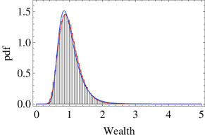
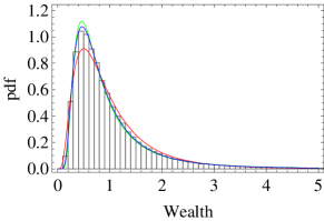
Figure 1: Histogram of “wealth” distribution for regular network with $z=0.01$ at $t=1$ (left) and $t=2500$ (right). Red: LN; Green: IGa; Blue: GIGa. The fitting of LN is good only for very short times. At $t=1$, the p-value of LN is 0.18; of IGa is 0; of GIGa is 0. At $t=2500$, the p-value of LN is 0; of IGa is 0; of GIGa is 0.05. For $t\geq 2$, the p-value of LN is always 0.

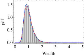
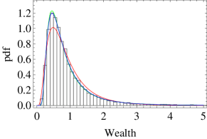
Figure 2: Histogram of “wealth” distribution for random small world network with $p_{SW}=0.003$ at $t=1$ (left) and $t=500$ (right). Red: LN; Green: IGa; Blue: GIGa. The fitting of LN is good only for very short times. At $t=1$, the p-value of LN is 0.51; of IGa is 0; of GIGa is 0. At $t=500$, the p-value of LN is 0; of IGa is 0.006; of GIGa is 0.97. For $t\geq 3$, the p-value of LN is always 0.

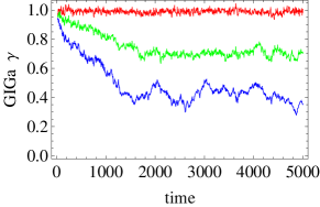
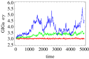
Figure 3: Regular network. First row: $\gamma$ of GIGa (colored), $\alpha\gamma$ of GIGa (colored). Red, green, and blue for $z=0.1,0.01,0.003$ respectively. Second, third, and fourth rows (uncolored) are p-values for $z=0.1,0.01,0.003$ respectively.

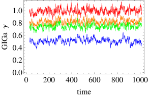
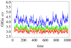
Figure 4: Random small world network. First row: $\gamma$ of GIGa (colored), $\alpha\gamma$ of GIGa (colored). Red, orange, green, and blue for $p_{SW}=0.1,0.003,0.002,0.001$ respectively. Second, third, fourth and fifth rows (uncolored) are p-values for $p_{SW}=0.1,0.003,0.002,0.001$

respectively.

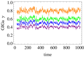
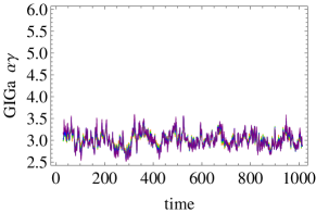
Figure 5: Effective field theory. First row: $\gamma$ of GIGa (colored), $\alpha\gamma$ of GIGa (colored). Orange, green, blue, and purple for $\gamma_{EFT}=0.8,0.6,0.5,0.4$ respectively. Second, third, fourth and fifth rows (uncolored) are p-values for $\gamma_{EFT}=0.8,0.6,0.5,0.4$ respectively.

IV Discussion

We demonstrated that the stationary solution of the partially connected Bouchaud-Mézard network model of the economy predicts the generalized inverse gamma distribution of “wealth.” In the mean-field limit of a fully connected network, we recover the inverse gamma distribution obtained in bouchaud2000 . Interestingly, the generalized inverse gamma also describes well the distribution of human response times ma2012 . We speculate that for some cases where Pareto distribution is observed it could be, in fact, a power-law tail of a (generalized) inverse gamma distribution. For instance, the distribution function of landslide area in turcotte2004 .

We described partially connected networks using an effective field theory and showed that it describes a randomly connected small world network particularly well, including the transitory behavior. Applicability of random versus regular network may depend on the circumstance, given the wide relevance of BM model, ranging from psychology to economics.

An interesting extension of this work would be to study the Watts and Strogatz network model watts1998 , which has both clustering and small-worldness properties. (This model has already been discussed by Souma et al. souma2001 .) The Watts and Strogatz model is more realistic than RanN as any real economic network should reflect both clustering and small-worldness nature.

Appendix A Numerical simulation method

A comprehensive list of numerical simulation methods of SDEs is given in kloeden1992 . In this paper, RanN and EFT are simulated by Milstien’s method, which has one-order accuracy, and RegN is simulated by the order 1.5 strong Taylor scheme. Below we only present Milstien’s method, which can be found in jacobs2010 and kloeden1992 . In Milstien’s method, the SDE

$$dx\overset{I}{=}f(x,t)dt+g(x,t)dB,$$ (16)

is written into the difference equation

$$\Delta x=f\Delta t+g\Delta B+\frac{g}{2}\frac{\partial g}{\partial x}[(\Delta W)^{2}-\Delta t].$$ (17)

For the BM model, $g=\sqrt{2}\sigma w_{i}$, hence

$$\frac{g}{2}\frac{\partial g}{\partial w_{i}}=\sigma^{2}w_{i}$$ (18)

and

$$\Delta x=f\Delta t+g\Delta B+\sigma^{2}w_{i}[(\Delta B)^{2}-\Delta t].$$ (19)

- (1) V.M. Yakovenko and J.B. Rosser Jr. Colloquium: Statistical mechanics of money, wealth, and income. RMP, 81(4):1703, 2009.
- (2) J.P. Bouchaud and M. Mézard. Wealth condensation in a simple model of economy. Physica A, 282(3):536–545, 2000.
- (3) Y. Fujiwara, W. Souma, H. Aoyama, T. Kaizoji, and M. Aoki. Growth and fluctuations of personal income. Physica A, 321(3):598–604, 2003.
- (4) H. Aoyama, Y. Fujiwara, and Y. Ikeda. Econophysics And Companies: Statistical Life And Death In Complex Business Networks. Cambridge Univ Pr, 2010.
- (5) A. Y. Abul-Magd. Wealth distribution in an ancient egyptian society. PRE, 66(5):057104, 2002.
- (6) W. Souma, Y. Fujiwara, and H. Aoyama. Small-world effects in wealth distribution. ArXiv cond-mat/0108482, 2001.
- (7) Aaron Clauset, Cosma Rohilla Shalizi, M. E. J. Newman. Power-law distributions in empirical data. arXiv:0706.1062, 2007.
- (8) K. Jacobs. Stochastic Processes For Physicists: Understanding Noisy Systems. Cambridge Univ Pr, 2010.
- (9) Weibull.com. The Generalized Gamma Distribution and Reliability Analysis http://www.weibull.com/hotwire/issue15/hottopics15.htm .
- (10) J.F. Lawless and JF Lawless. Statistical models and methods for lifetime data. 1982.
- (11) M. Evans, N. Hastings, and B. Peacock. Statistical distributions. 2000.
- (12) D.J. Watts and S.H. Strogatz. Collective dynamics of ‘small-world’ networks. Nature, 393(6684):440–442, 1998.
- (13) Gavin E. Crooks. The Amoroso Distribution arXiv:1005.3724v1, 2010
- (14) Peter E. Kloeden and Eckhard Platen. Numerical Solution of Stochastic Differential Equations. Springer-Verlag, 1992.
- (15) Tao Ma, R. A. Serota and John G. Holden (unpublished)
- (16) Donald L. Turcotte, Bruce D. Malamud Landslides, forest fires, and earthquakes: examples of self-organized critical behavior Physica A, 340:580–589, 2004.