F-Theory and the Mordell-Weil Group
of Elliptically-Fibered Calabi-Yau Threefolds

Abstract:

The Mordell-Weil group of an elliptically fibered Calabi-Yau threefold $X$ contains information about the abelian sector of the six-dimensional theory obtained by compactifying F-theory on $X$. After examining features of the abelian anomaly coefficient matrix and $U(1)$ charge quantization conditions of general F-theory vacua, we study Calabi-Yau threefolds with Mordell-Weil rank-one as a first step towards understanding the features of the Mordell-Weil group of threefolds in more detail. In particular, we generate an interesting class of F-theory models with $U(1)$ gauge symmetry that have matter with both charges $1$ and $2$. The anomaly equations — which relate the Néron-Tate height of a section to intersection numbers between the section and fibral rational curves of the manifold — serve as an important tool in our analysis.

1 Introduction and Summary

The abelian sector of F-theory backgrounds is interesting from at least two different points of view. From the point of view of F-theory phenomenology, understanding how to protect and break various $U(1)$’s in F-theory model building is essential to constructing models with desired properties. Meanwhile, from the point of view of addressing the question of 6D string universality [7], a systematic understanding of what one could get in string theory — especially F-theory — is crucial. Such an understanding of the abelian sector of F-theory has yet to be gained. In this note, we approach abelian gauge symmetry from the latter viewpoint.

The six-dimensional string universality conjecture is the conjecture that all “consistent” six-dimensional supergravity theories with minimal supersymmetry are embeddable in string theory [7]. Much progress has been made on verifying this conjecture by focusing on theories with non-abelian gauge symmetry [8, 9, 10, 11]. Much more, however, needs to be understood upon introducing abelian gauge symmetry to the picture [12].

In particular, it is not well understood what kind of $U(1)$ charges are allowed in F-theory. A simple version of the problem is to ask what kind of charges are allowed for the matter of a six-dimensional F-theory background whose gauge group is given by $\mathcal{G}=U(1)$. We currently do not know the answer even to this seemingly innocent problem. In this note, we take some first steps towards improving the current status.

The abelian sector of six-dimensional F-theory backgrounds — obtained by compactification on an elliptically fibered Calabi-Yau threefold $X$ [13, 14] — contains information about the Mordell-Weil group of the threefold $X$. In particular, the rank of the abelian gauge group is equal to the Mordell-Weil rank [14], while the anomaly coefficient matrix of the abelian gauge fields turns out to be the Néron-Tate height pairing matrix of the Mordell-Weil generators [15]. Therefore, in order to understand the abelian sector of supersymmetric F-theory backgrounds, one must study the Mordell-Weil group of elliptically fibered Calabi-Yau manifolds.

The Mordell-Weil group of an elliptic fibration — which is the group of rational sections of the fibration — is a rather elusive mathematical object to study. We make an initial step in this note to understand the Mordell-Weil group of an elliptically fibered Calabi-Yau threefold from the point of view of F-theory. In particular, we focus on a very simple class of manifolds — namely, Calabi-Yau threefolds fibered over ${\mathbb{{P}}}^{2}$ with no enhanced gauge symmetry and Mordell-Weil rank-one. Compactification of F-theory on such a manifold yields a six-dimensional supergravity theory with no tensor multiplets and gauge group $U(1)$. We concern ourselves with understanding what kind of charges of matter are allowed for such theories.

Strong constraints on the non-abelian sector of six-dimensional F-theory backgrounds are imposed by the Kodaira condition [26, 27, 28, 29, 30]. The Kodaira condition “bounds” the anomaly coefficients associated to each non-abelian gauge group, which in turn restricts the matter representations charged under the non-abelian gauge groups. Similar bounds on the height-pairing matrix of the Mordell-Weil generators, if they exist, would lead to constraints on charges of the abelian sector.

Let us summarize the main results of this note.

1. We explicitly compute the height pairing matrix of a given set of Mordell-Weil generators and discuss their properties for general Calabi-Yau threefolds.

   • In particular, the self-height pairing of the Mordell-Weil generator ${\hat{s}}$ of a Calabi-Yau threefold fibered over ${\mathbb{{P}}}^{2}$ with Mordell-Weil rank-one is parameterized by a single non-negative integer $n$, in the absence of enhanced non-abelian gauge symmetry. A bound on this number $n$ would serve as an analogue of the Kodaira bound for these theories.

2. Using anomalies, we show that when one assumes that the charge of the matter is either $1$ or $2$ there are only nine distinct possible theories each with $n=0,\cdots,8$.

3. We explicitly construct seven of these nine theories, namely theories with $n=0,\cdots,6$.

The structure of this note is as the following. We first review six-dimensional F-theory backgrounds in section 2. We then compute the abelian anomaly coefficients of an F-theory background after reviewing how to extract information of the abelian sector of F-theory models from the geometry in section 3, i.e., we arrive at result (1). In particular, we show how the analysis simplifies in the case of pure abelian theories with no tensor multiplets. In section 4, we show how the charge is restricted in the case of pure abelian models with no tensor multiplets when the anomaly coefficient is given. In particular, we reach result (2) in this section. We construct specific models with Mordell-Weil rank $1$ in more detail in section 5, i.e., we arrive at result (3). We sketch questions and future directions in section 6.

2 Review of Six-Dimensional Supergravity Theories

We review relevant facts about six-dimensional $(1,0)$ supergravity theories and F-theory backgrounds in this section. We also explain why the Kodaira condition restricts the charged matter structure for the non-abelian sector of F-theory models briefly. The presentation of this section is rather condensed. Further details can be found in [12, 15].

Multiplet	Field Content
Gravity	$(g_{\mu\nu},\psi^{+}_{\mu},B^{+}_{\mu\nu})$
Tensor	$(\phi,\chi^{-},B^{-}_{\mu\nu})$
Vector	$(A_{\mu},\lambda^{+})$
Hyper	$(4\varphi,\psi^{-})$

Table 1: Six-dimensional (1,0) supersymmetry multiplets. The signs on the fermions indicate the chirality. The signs on antisymmetric tensors indicate self-duality/anti-self-duality.

The low-energy data of six-dimensional supergravity theories can be parameterized by its massless spectrum $S$, anomaly coefficients $\{b\}$ and a “modulus” $j$. The massless particles come in BPS multiplets of the $(1,0)$ supersymmetry algebra given in table 1. The massless spectrum $S$ is specified by the number of tensor multiplets $T$, the (global) gauge group

$$\mathcal{G}=\prod_{\kappa=1}^{n}\mathcal{G}_{\kappa}\times\prod_{i=1}^{V_{A}}U(1)_{i}$$ (1)

— where $\mathcal{G}_{\kappa}$ are simple non-abelian gauge group factors — and the matter representation of the hypermultiplets. ${V_{A}}$ denotes the number of abelian gauge group factors. There is one gravity multiplet in the theory.

The anomaly coefficients $\{b\}$ are a set of $SO(1,T)$ vectors. To each non-abelian gauge group factor $\mathcal{G}_{\kappa}$, there is an $SO(1,T)$ vector $b_{\kappa}$ associated to it, which we call the “anomaly coefficient of $\mathcal{G}_{\kappa}$.” For the abelian sector, there is an associated ${V_{A}}\times{V_{A}}$ matrix $b_{ij}$ whose components are also $SO(1,T)$ vectors. We call this matrix the “abelian anomaly coefficient matrix.” Abelian vector fields are defined only up to linear transformations. Imposing charge minimality constraints on the abelian gauge symmetry, the abelian gauge fields are defined up to $SL({V_{A}},{\mathbb{{Z}}})$ — it follows that $b_{ij}$ transforms as a bilinear under this $SL({V_{A}},{\mathbb{{Z}}})$. There also exists a gravitational anomaly coefficient $a$ that is needed to cancel the gravitational/mixed anomalies of the theory.

These six-dimensional theories must satisfy generalized Green-Schwarz anomaly cancellation conditions [33, 34, 35, 36, 37, 38]. These anomaly cancellation conditions come from imposing that the eight-dimensional anomaly polynomial — computed by adding the contribution of all the chiral fields of the theory [39, 40, 41] — should factor into the form

$$I_{8}\propto({1\over 2}a{\rm tr}R^{2}+\sum_{\kappa}{2b_{\kappa}\over\lambda_{\kappa}}{\rm tr}F_{\kappa}^{2}+\sum_{i,j}2b_{ij}F_{i}F_{j})^{2}$$ (2)

where the norm is taken with respect to an $SO(1,T)$ metric ${\Omega}_{\alpha\beta}$. $\lambda_{\kappa}$ is the Dynkin index of the fundamental representation of $\mathcal{G}_{\kappa}$. The explicit form of the anomaly equations have been written out, for example, in [10, 12, 15, 42, 43] and we do not reproduce them here.

The anomaly coefficients, along with the modulus $j$ determine important terms in the low-energy effective Lagrangian. The modulus $j$ is a unit $SO(1,T)$ vector parametrizing the vacuum expectation value of the $T$ scalar fields in the tensor multiplets. In particular, they determine the kinetic terms for the gauge fields

$$\propto\sum_{\kappa}({j\cdot b_{\kappa}\over\lambda_{\kappa}}){\rm tr}F_{\kappa}\wedge*F_{\kappa}+\sum_{k,l}({j\cdot b_{kl}})F_{k}\wedge*F_{l}\,,$$ (3)

and the Green-Schwarz term

$$\propto B\cdot({1\over 2}a{\rm tr}R^{2}+\sum_{\kappa}{2b_{\kappa}\over\lambda_{\kappa}}{\rm tr}F_{\kappa}^{2}+\sum_{i,j}2b_{ij}F_{i}F_{j})\,,$$ (4)

where the self-dual and anti-self-dual tensors are organized into an $SO(1,T)$ vector and the inner-product is taken with respect to ${\Omega}_{\alpha\beta}$.

A six-dimensional $(1,0)$ supergravity theory can be obtained by compactifying F-theory on an elliptically fibered Calabi-Yau threefold ${\hat{X}}$ with a section. The anomaly coefficients have a nice interpretation in terms of the geometry of ${\hat{X}}$. In particular, the $SO(1,T)$ lattice on which the anomaly coefficients live is the $H_{2}$ homology lattice of the base ${\cal B}$ of the fibration. The base ${\cal B}$ of the fibration must be a rational surface with $h^{1,1}({\cal B})=T+1$. The anomaly coefficients turn out to be curves — i.e., divisors — on the base which are represented by vectors in the homology lattice $H_{2}({\cal B})$. In particular, the gravitational anomaly coefficient $a$ corresponds to the canonical divisor while the coefficient $b_{\kappa}$ corresponds to the degeneration locus of the fiber that yields the $\mathcal{G}_{\kappa}$ gauge symmetry [9, 10, 13, 14, 44].

The abelian anomaly coefficients can be obtained in the following way. Each abelian gauge field corresponds to a generator of the Mordell-Weil group of the elliptic fibration. The Mordell-Weil group is the group of rational sections of the fibration, and is generated by a finite basis. The basis is defined up to $SL({V_{A}},{\mathbb{{Z}}})$, which is precisely the group of redefinitions on $U(1)$’s preserving charge minimality. Denoting the the basis elements of the Mordell-Weil group $\{{\hat{s}}_{1},\cdots,{\hat{s}}_{V_{A}}\}$, the abelian anomaly coefficients are given by

$$b_{ij}=-\pi(\sigma({\hat{s}}_{i})\cdot\sigma({\hat{s}}_{j}))\,.$$ (5)

Some explanation of notation is due. $\sigma$ is a map from the Mordell-Weil group to $H_{4}({\hat{X}})$ defined by Shioda in [45], which we refer to as the Shioda map. We explain this map in more detail in the subsequent section, but mention here that it is a homomorphism from the Mordell-Weil group to the homology group $H_{4}$. In other words, the group action — or addition — of sections carry over to into addition of the homology class of the corresponding sections under the Shioda map [45, 46]. The dot product is the intersection product in the manifold $X$. $\pi(C)$ is defined as the projection of a curve $C$ to the base ${\cal B}$. At the operational level, if we denote by $B_{\alpha}$ the pullback of the generators $H_{\alpha}$ of the base homology by the projection map, $\pi$ is defined by

$$\pi(C)=(C\cdot B_{\alpha})H^{\alpha}\,.$$ (6)

Here the $\alpha$ indices are vector indices of the base homology lattice. They are raised and lowered by the metric

$${\Omega}_{\alpha\beta}=H_{\alpha}\cdot H_{\beta}\,,$$ (7)

where the intersection product is taken within the base manifold in this equation.

In order for the fibration to be Calabi-Yau, the Kodaira equality

$$-12a=\sum_{\kappa}\nu_{\kappa}b_{\kappa}+Y$$ (8)

must hold for some effective divisor $Y$, where $\nu_{\kappa}$ are coefficients associated to the reducible fiber at $b_{\kappa}$. Numerical values for $\nu_{\kappa}$ can be found in, for example, [13]. The Kodaira equality can also be thought of as a bound

$$-12a\geq\sum_{\kappa}\nu_{\kappa}b_{\kappa}\,,$$ (9)

i.e., it bounds the anomaly coefficients in a given base above by $-12a$. When there are hypermultiplets of representations with large charges under the gauge group $\mathcal{G}_{\kappa}$, the values $b_{\kappa}\cdot b_{\kappa}$, $b_{\kappa}\cdot b_{\lambda}$ and $a\cdot b_{\kappa}$ become large. The Kodaira bound therefore restricts the representations allowed in F-theory models by bounding $b_{\kappa}$. Such restrictions placed by the Kodaira bound have been explicitly demonstrated in the case of $T=0$ models in [11].

Meanwhile, an analogous constraint on the abelian anomaly coefficient has yet to be found. Such a constraint would also restrict the allowed charge of matter in F-theory models. For example, by anomaly cancellation,

$$b_{ii}\cdot b_{ii}={1\over 3}\sum_{q}x_{q}q^{4}$$ (10)

where $x_{q}$ is the number of hypermultiplets with charge $q$ under $U(1)_{i}$. A bound on $b_{ii}$ would restrict the charges hypermultiplets can have, given that there is a unit of quantization of the $U(1)$ charges. We explore such restrictions further in section 4.

3 The Abelian Sector of F-theory Vacua

In this section, we review how to extract data on the abelian sector of F-theory vacua and examine the special case of $T=0$ backgrounds with gauge group $U(1)$ in detail. In section 3.1, we give a general overview of the Mordell-Weil group of an elliptically fibered Calabi-Yau threefold and its relation to the abelian sector of the corresponding six-dimensional F-theory background. We specialize to F-theory backgrounds with $T=0$ and gauge group $U(1)$ in section 3.2.

3.1 The Mordell-Weil Group and the Abelian Sector of F-theory

In this section, we review relevant facts about the Mordell-Weil group of elliptic fibrations and its relation to the abelian sector of F-theory backgrounds. A more thorough description of the process of extracting the physical data of six-dimensional F-theory backgrounds can be found in [15, 47]. More information on elliptic curves and the Mordell-Weil group can be found in standard introductory texts on the subject, such as [48].

Six-dimensional F-theory compactifications are defined for elliptically fibered Calabi-Yau threefolds with a section. Let us denote such a smooth elliptic fibration by ${\hat{X}}$ and its base manifold by ${\cal B}$. Such manifolds have a Weierstrass representation

$$X~{}:\quad y^{2}=x^{3}+fxz^{4}+gz^{6}\,.$$ (11)

$f$ and $g$ are holomorphic sections of the line bundles $-4K$ and $-6K$ respectively, where $K$ is the canonical class of the base manifold. Hence the Calabi-Yau threefold can be thought of as an elliptic curve over a function field. Given an elliptic curve over a field with a choice of a “zero point” there is an abelian group operation — which we denote by “${[+]}$” — on the points of the elliptic curve. This operation is defined in appendix A.

The rational sections of the fibration can be thought of as rational points on the elliptic curve over the function field of the base ${\cal B}$. As elaborated in appendix A, these points form an abelian group under ${[+]}$. This group is called the Mordell-Weil group of the elliptic curve.

The Mordell-Weil theorem states that this group is finitely generated. (Unfortunately, the proof does not provide an algorithm for computing it!) Any finitely generated abelian group can be written in the form

$${\mathbb{{Z}}}\oplus\cdots\oplus{\mathbb{{Z}}}\oplus\mathcal{G}$$ (12)

where $\mathcal{G}$ is the torsion subgroup. Let us denote by $\{{\hat{s}}_{1},\cdots,{\hat{s}}_{V_{A}}\}$ a set of rational sections that generate the non-torsion part of the Mordell-Weil group, i.e., a “basis” of the Mordell-Weil group. As mentioned in the previous section, this basis is defined up to linear redefinitions $SL({V_{A}},{\mathbb{{Z}}})$. ${V_{A}}$ is called the Mordell-Weil rank.

Let us denote the homology classes of the sections $\{{\hat{s}}_{1},\cdots,{\hat{s}}_{V_{A}}\}$ — which are four-cycles within the threefold — by $\{{\hat{S}}_{1},\cdots,{\hat{S}}_{V_{A}}\}$. In fact, we frequently denote a rational section by a hatted lower-case roman letter and its homology class by the corresponding hatted upper-case letter throughout this note. The Shioda-Tate-Wazir theorem [49] states that $\{{\hat{S}}_{1},\cdots,{\hat{S}}_{V_{A}}\}$ along with the zero section $Z$, the vertical divisors $B_{\alpha}$ and the “fibral divisors” $T_{\kappa,I}$ generate the homology group $H_{4}({\hat{X}})$. The fibral divisors of ${\hat{X}}$ are topologically rational curves fibered over codimension-one loci $b_{\kappa}$ of the base.

The structure of the fibral divisors determine the non-abelian gauge group and anomaly coefficients. Each non-abelian gauge group $\mathcal{G}_{\kappa}$ is associated to a curve/divisor $b_{\kappa}$ in the base manifold where the fiber becomes degenerate. The irreducible components of the degenerate fibers are generated by a set of rational curves $\alpha_{\kappa,I}$ that correspond to the simple roots of the Lie algebra $\mathcal{G}_{\kappa}$. Any rational curve that is a fiber component along $b_{\kappa}$ can be written as a linear combination of $\alpha_{\kappa,I}$ — these rational curves correspond to the positive roots of the Lie algebra $\mathcal{G}_{\kappa}$. The fibral divisors $T_{\kappa,I}$ are obtained by fibering these rational curves $\alpha_{\kappa,I}$ over the locus $b_{\kappa}$. The monodromy invariant fiber of $T_{\kappa,I}$, which we denote by $\gamma_{\kappa,I}$ — can consist of multiple rational curves.

Let us digress briefly to describe degenerate fibers of the manifold. The rational curve components of degenerate fibers shrink in the “F-theory limit” and contribute massless vector and hypermultiplets to the six-dimensional spectrum. This is equivalent to saying that these rational curves satisfy

$$c\cdot Z=c\cdot B_{\alpha}=0\,.$$ (13)

We call the fibral rational curves — rational curves that are components of a degenerate fiber — that are fibered over some curve in the base $b_{\kappa}$, “fibered” (fibral) rational curves. Each fibered rational curve contributes two vector multiplets and $2g$ hypermultiplets to the massless spectrum, where $g$ is the genus of the curve the rational curve is fibered over. There can be other fibral rational curves that are isolated at codimension-two loci in the base. We call these “isolated” (fibral) rational curves. Each of these curves contribute a hypermultiplet to the six-dimensional spectrum. For obvious reasons, we use the term “fibral rational curves” and “shrinking rational curves” interchangeably.

Now we are in a position to define the Shioda map $\sigma$. For a rational section ${\hat{s}}$, let ${\hat{S}}\in H_{4}({\hat{X}})$ be its homology class. Then

$$\sigma({\hat{s}})={\hat{S}}-Z-({\hat{S}}\cdot Z\cdot B^{\alpha}-K^{\alpha})B_{\alpha}+\sum_{I,J,\kappa}({\hat{S}}\cdot\alpha_{\kappa,I})(C_{\kappa}^{-1})_{IJ}T_{\kappa,J}\,.$$ (14)

Here $K^{\alpha}$ are the coordinates of the canonical class of the base, while $C_{\kappa}$ is the Cartan matrix of the Lie algebra $\mathcal{G}_{\kappa}$ defined by

$$(C_{\kappa})_{IJ}={2\langle\alpha_{I},\alpha_{J}\rangle\over\langle\alpha_{I},\alpha_{I}\rangle}$$ (15)

where $\alpha_{I}$ are the simple roots of $\mathcal{G}_{\kappa}$. There is a one-to-one correspondence between the abelian vector fields $\{A_{1},\cdots,A_{V_{A}}\}$ and the four-cycles $\{\sigma({\hat{s}}_{1}),\cdots,\sigma({\hat{s}}_{V_{A}})\}$. For convenience we say that $A_{i}$ is “dual to” $\sigma({\hat{s}}_{i})$. The anomaly coefficient matrix is given by

$$b_{ij}=-\pi(\sigma({\hat{s}}_{i})\cdot\sigma({\hat{s}}_{j}))$$ (16)

where $\pi$ is the projection to the $H_{2}({\cal B})$ homology lattice of the base. As we elaborate shortly, this is the generalized Néron-Tate height pairing for elliptically fibered threefolds, and $b_{ij}$ constitutes the height pairing matrix of the elliptic fibration.

Let us briefly review the mathematical significance of the Shioda map. For elliptically fibered Calabi-Yau threefolds, there is a natural inner-product on two elements $S,S^{\prime}$ of $H_{4}({\hat{X}},{\mathbb{{Z}}})\cong H^{2,2}({\hat{X}})$ with values in $H_{2}({\cal B})$ [49]. It is, in fact, given by

$$\begin{split}\langle~{},~{}\rangle~{}:~{}H_{4}({\hat{X}})\times H_{4}({\hat{X}})\quad&\rightarrow\quad H_{2}({\cal B})\\ (S,S^{\prime})\quad&\mapsto\quad-\pi(S\cdot S^{\prime})\end{split}$$ (17)

The Shioda map $\sigma$ is the map from the Mordell-Weil group to the orthogonal complement of the space spanned by the zero section $Z$, the vertical divisors $B_{\alpha}$ and the fibral divisors $T_{\kappa,I}$ under this inner-product. In other words,

$$\langle\sigma({\hat{s}}),C\rangle=0$$ (18)

for any section ${\hat{s}}$ and an element $C$ which is an element of the subspace of $H_{4}({\hat{X}})$ spanned by $Z$, $B_{\alpha}$ and $T_{I,\kappa}$. Following [46], let us denote this subspace by “$T$.” Using the fact that $\sigma({\hat{s}})$ is a projection of the homology class of ${\hat{s}}$ to $H_{4}(X)/T$, it can be shown that $\sigma$ is a homomorphism from the Mordell-Weil group to the homology lattice [45, 46, 49], i.e.,

$$\sigma({\hat{s}}{[+]}{\hat{s}}^{\prime})=\sigma({\hat{s}})+\sigma({\hat{s}}^{\prime})\,,$$ (19)

where the addition on the right-hand-side is the addition defined for the homology group. Then, the inner-product

$$\langle\sigma({\hat{s}}),\sigma({\hat{s}}^{\prime})\rangle=-\pi(\sigma({\hat{s}})\cdot\sigma({\hat{s}}^{\prime}))$$ (20)

is the Néron-Tate height pairing of rational sections of the elliptic fibration.

As mentioned previously, each abelian vector field $A_{i}$ is dual to $\sigma({\hat{s}}_{i})$. Also, each element of the Cartan of the non-abelian gauge group $\mathcal{A}_{\kappa,I}$ is dual to the fibral divisors $T_{\kappa,I}$ in the same sense. A multiplet coming from a fibral rational curve $c$ has charge $S\cdot c$ under the Cartan vector field dual to a four-cycle $S$.

By construction $\sigma({\hat{s}}_{i})\cdot c=0$ for any fibered rational curve $c$, and therefore no vector multiplet is charged under the abelian vector fields $A_{i}$, as desired. Hence only hypermultiplets coming from isolated rational curves are charged under the abelian vector fields. For any isolated rational curve $c$, the hypermultiplet corresponding to it has charge

$$\sigma({\hat{s}}_{i})\cdot c=({\hat{S}}_{i}\cdot c)+\sum_{I,J,\kappa}({\hat{S}}_{i}\cdot\alpha_{\kappa,I})(C_{\kappa}^{-1})_{IJ}(T_{\kappa,J}\cdot c)\,.$$ (21)

under $A_{i}$. Since the intersection numbers $({\hat{S}}_{i}\cdot c)$ and $(T_{\kappa,J}\cdot c)$ are integral, we see that the unit charge of the abelian vector field $A_{i}$ is given by the inverse of the least common multiple of $\{{\rm det}(C_{\kappa})\}$, where $\kappa$ runs over the gauge groups for which $\alpha_{I,\kappa}\cdot{\hat{S}}_{i}\neq 0$ for some root $\alpha_{I,\kappa}$. In particular, when $c\cdot{\hat{S}}_{i}=0$ for all fibered rational curves $c$, the charges of the matter under the abelian vector fields are integral.

Let us end this section by computing the abelian anomaly coefficient matrix and examining its properties. The anomaly coefficient matrix can be written as

$$b_{ij}=-\pi({\hat{S}}_{i}\cdot{\hat{S}}_{j})-K+(n_{i}+n_{j})-(\mathcal{R}^{-1}_{\kappa})_{IJ}({\hat{S}}_{i}\cdot\alpha_{I,\kappa})({\hat{S}}_{j}\cdot\alpha_{J,\kappa})b_{\kappa}\,.$$ (22)

$n_{i}$ is the locus along which section $S_{i}$ intersects the zero section, i.e.,

$$n_{i}\equiv\pi({\hat{S}}_{i}\cdot Z)\,.$$ (23)

$K$ is the canonical class of the base manifold. The matrix $\mathcal{R}_{\kappa}$ is the normalized root matrix of Lie group $\mathcal{G}_{\kappa}$

$$(\mathcal{R}_{\kappa})_{IJ}={2\langle\alpha_{I},\alpha_{J}\rangle\over\langle\alpha,\alpha\rangle_{\text{max}}}$$ (24)

where $\langle\alpha,\alpha\rangle_{\text{max}}$ is the length of the longest root of the Lie group. We have used the following equalities in arriving at (22):

$$Z\cdot Z\cdot B_{\alpha}=K_{\alpha},\quad Z\cdot B_{\alpha}\cdot B_{\beta}={\hat{S}}\cdot B_{\alpha}\cdot B_{\beta}={\Omega}_{\alpha\beta},\quad Z\cdot f={\hat{S}}\cdot f=1\,.$$ (25)

The first of these equations follow from the adjunction formula, and the Calabi-Yau condition — by these two facts, the canonical class of $Z$ is given by the restriction of the divisor class $Z$ to itself, and hence

$$Z\cdot Z\cdot B_{\alpha}=Z|_{Z}\cdot H_{\alpha}=K\cdot H_{\alpha}=K_{\alpha}\,,$$ (26)

since $Z$ is topologically just the base manifold. The intersection products in the second and third terms are taken in the base manifold $Z$.

Such a relation actually holds for any section ${\hat{S}}$, i.e.,

$${\hat{S}}\cdot{\hat{S}}\cdot B_{\alpha}={\hat{S}}|_{\hat{S}}\cdot H_{\alpha}=K\cdot H_{\alpha}=K_{\alpha}\,.$$ (27)

In general, ${\hat{S}}$ is topologically a manifold obtained by blowing up points on the base manifold ${\cal B}$. Its $H_{\alpha}$ components, however, coincide with those of the canonical class of the base manifold. Therefore

$$b_{ii}=-2K+2n_{i}-(\mathcal{R}^{-1}_{\kappa})_{IJ}({\hat{S}}_{i}\cdot\alpha_{I,\kappa})({\hat{S}}_{i}\cdot\alpha_{J,\kappa})b_{\kappa}\,.$$ (28)

$\mathcal{R}_{\kappa}$ is clearly a positive-definite matrix and since $b_{\kappa}$ is effective, it can be further seen that

$$b_{ii}\leq-2K+2n_{i}\,.$$ (29)

3.2 $T=0$ Theories with Gauge Group $U(1)$

In this section, we specialize to F-theory backgrounds with $T=0$ and gauge group $U(1)$ and examine the abelian sector. The abelian charges in this case turn out to be quantized to be integers. Also, the abelian anomaly coefficient is parametrized by a single integer $n$.

Six-dimensional $T=0$ theories are obtained by F-theory compactifications on an elliptically fibered Calabi-Yau manifold over ${\mathbb{{P}}}^{2}$. As $h^{1,1}({\mathbb{{P}}}^{2})=1$, $H^{2}({\cal B})$ is generated by the hyperplane class $H$. There is only one vertical divisor, $B$, obtained by pulling back the hyperplane class with respect to the projection map. As the homology lattice of the base is one-dimensional, the anomaly coefficients of the theory — being vectors in this lattice — are numbers.

If we restrict our attention to theories with gauge group $U(1)$, the situation simplifies further. The $H_{4}({\hat{X}})$ lattice is generated by the zero section $Z$, the vertical divisor $B$, and $S\equiv\sigma({\hat{s}})$ where ${\hat{s}}$ is the generator of the Mordell-Weil group. All the fibral rational curves are isolated. It is clear that the unit charge for the abelian vector field is $1$ by the discussion in the last subsection, as there are no fibral divisors.

The Shioda map simplifies to

$$\sigma({\hat{s}}^{\prime})={\hat{S}}^{\prime}-Z-({\hat{S}}^{\prime}\cdot Z\cdot B+3)B$$ (30)

for any rational section ${\hat{s}}^{\prime}$. ${\hat{S}}^{\prime}$ is the homology class of ${\hat{s}}^{\prime}$. We have used

$$Z\cdot Z\cdot B=Z|_{Z}\cdot B|_{Z}=K\cdot H=-3\,,$$ (31)

which follows from the adjunction formula and the fact that the canonical class of the base is given by $K=-3H$.

The Weierstrass model for this elliptic fibration is given by

$$X~{}:\quad y^{2}=x^{3}+F_{12}xz^{4}+G_{18}z^{6}$$ (32)

where $F_{12}$ and $G_{18}$ are holomorphic sections of $12H$ and $18H$. The Mordell-Weil generator ${\hat{s}}$ must have the form

$${\hat{s}}~{}:~{}[x,y,z]=[f_{2n+6},f_{3n+9},f_{n}],$$ (33)

for mutually relatively prime polynomials $f_{2n+6}$, $f_{3n+9}$ and $f_{n}$. $f_{k}$ are polynomials of degree $k$ with respect to the ${\mathbb{{P}}}^{2}$ coordinates. Then it is clear that the intersection of this section with $Z$ is at $nH$, i.e.,

$${\hat{S}}\cdot Z\cdot B=n\,.$$ (34)

The Shioda map maps the section to

$$S=\sigma({\hat{s}})={\hat{S}}-Z-(n+3)B\,.$$ (35)

The abelian anomaly coefficient matrix has the single component

$$b=-S\cdot S\cdot B=6+2{\hat{S}}\cdot Z\cdot B=2(n+3)\,.$$ (36)

Therefore the anomaly coefficient is determined by a single number $n$, which parametrizes the degree of the curve on which ${\hat{s}}$ intersects the zero-section.

As mentioned earlier, all the fibral curves are isolated. Each isolated rational curve $c$ corresponds to a hypermultiplet of the six-dimensional theory. The charge of the hypermultiplet under the abelian gauge group is given by the intersection number

$$c\cdot\sigma({\hat{s}})=c\cdot{\hat{S}}\,.$$ (37)

As mentioned at various points in this note, understanding the bounds on $b$ is crucial in understanding what kind of charges are allowed in F-theory. For F-theory backgrounds with $T=0$ and gauge group $U(1)$, we have shown that the charges are integral and that $b=2(n+3)$ when the generator of the Mordell-Weil group is of the form

$${\hat{s}}~{}:~{}[x,y,z]=[f_{2n+6},f_{3n+9},f_{n}]\,.$$ (38)

Therefore the interesting question is what the bound on the integer $n$ is. Such a bound would play — in $U(1)$ theories — the role the Kodaira bound plays in restricting non-abelian theories.

We note that given any elliptically fibered Calabi-Yau manifold of Mordell-Weil rank $\geq 1$, there exists a section with arbitrarily large self-height pairing, which can be obtained by adding a given rational section many times. Let us demonstrate this fact. Given any section

$${\hat{s}}^{\prime}~{}:~{}[x,y,z]=[f_{2n+6},f_{3n+9},f_{n}]\,,$$ (39)

and its homology class ${\hat{S}}^{\prime}$, one can show that the homology class ${\hat{S}}^{\prime}_{m}$ of $m{\hat{s}}^{\prime}$ is given by

$${\hat{S}}^{\prime}_{m}=m{\hat{S}}^{\prime}-(m-1)Z-(n+3)m(m-1)B\,.$$ (40)

To show this, one begins with the fact that

$$\sigma(m{\hat{s}}^{\prime})=m\sigma({\hat{s}}^{\prime})=m{\hat{S}}^{\prime}-mZ-m(n+3)B$$ (41)

and hence

$${\hat{S}}^{\prime}_{m}=m{\hat{S}}^{\prime}-zZ-bB\,,$$ (42)

for some $z$ and $b$. Since $m{\hat{s}}^{\prime}$ is also a section, its homology class ${\hat{S}}^{\prime}_{m}$ intersects the fiber class once. Imposing that ${\hat{S}}^{\prime}_{m}\cdot f=1$ for the fiber class $f$, one obtains $z=(m-1)$. Finally imposing the condition that

$${\hat{S}}^{\prime}_{m}\cdot{\hat{S}}^{\prime}_{m}\cdot B=-3\,,$$ (43)

one arrives at (40). Since

$${\hat{S}}^{\prime}_{m}\cdot Z\cdot B=mn+3(m-1)-(n+3)m(m-1)=(n+3)m^{2}-3,$$ (44)

the section $m{\hat{s}}^{\prime}$ is of the form

$$m{\hat{s}}^{\prime}~{}:~{}[x,y,z]=[f_{2(n+3)m^{2}},f_{3(n+3)m^{2}},f_{(n+3)m^{2}-3}]\,,$$ (45)

with self-height pairing

$$-\pi(\sigma(m{\hat{s}}^{\prime})\cdot\sigma(m{\hat{s}}^{\prime}))=2(n+3)m^{2}\,.$$ (46)

The relevant question to ask is what the bound to the height of a Mordell-Weil generator is. We do not know the answer to this question at the present. To address this question, one must first understand how to discern whether a section is a generator or not. We can do this in the case of pure $U(1)$ theories. More precisely put, a sufficient condition for a given section to be a Mordell-Weil generator is that the integral charges of the matter under the dual abelian vector field is mutually relatively prime. In geometric terms, given a section ${\hat{s}}^{\prime}$, the section ${\hat{s}}^{\prime}$ is a generator of the Mordell-Weil group when the set of intersection numbers of its homology class ${\hat{S}}^{\prime}$ (or equivalently $\sigma({\hat{s}}^{\prime})$) with the isolated rational curves of the manifold $c_{1},\cdots,c_{H}$ are mutually relatively prime. This is because if ${\hat{s}}^{\prime}=m{\hat{s}}$ for some ${\hat{s}}$ and $|m|>1$, ${\hat{S}}^{\prime}$ is given by

$${\hat{S}}^{\prime}=m{\hat{S}}-(m-1)Z-(n+3)m(m-1)B$$ (47)

where ${\hat{S}}$ is the homology class of ${\hat{s}}$. Therefore the intersection numbers of ${\hat{S}}^{\prime}$ with the isolated fibral rational curves $c_{1},\cdots,c_{H}$ are given by

$$q_{I}\equiv{\hat{S}}^{\prime}\cdot c_{I}=m({\hat{S}}\cdot c_{I})\,,$$ (48)

and hence $\{q_{I}\}$ have $m$ as a common divisor.

4 Anomaly Coefficients and Charge Constraints

In this section, we see how the anomaly coefficient of a $U(1)$ theory with $T=0$ constrains the charges of the matter. As seen in the previous sections, for F-theory backgrounds with $T=0$ and gauge group $U(1)$, the abelian anomaly coefficient matrix is given by $b=2(n+3)$ with non-negative integer $n$. The charges of matter under the given $U(1)$ represented by the Mordell-Weil generator are quantized to be integers. Hence the mixed/gauge anomaly equations are given by

$$18b=36(n+3) =\sum_{c=1}^{m}c^{2}n_{c}$$ (49)

$$3b^{2}=12(n+3)^{2} =\sum_{c=1}^{m}c^{4}n_{c}$$ (50)

where $n_{c}$ is the number of matter with charge $c$ and $m$ is the maximal charge. The gravitational anomaly bound is given by

$$\sum_{c=1}^{m}n_{c}\leq 274\,.$$ (51)

It is clear from these equations that

$$m^{2}\geq{n\over 3}+1\,,$$ (52)

i.e., that when $n$ is large, there must be some matter with charge at least $\sqrt{(n+3)/3}$. The converse, obviously, does not hold. For example, one could have theories with $n<9$ that have matter with charge $3$. It is possible to show, however, that when $b=6$, the only possible choice of matter content is that there are $108$ hypermultiplets of charge $1$.

It is interesting to classify all the possible theories with only charges $1$ and $2$. The theories are characterized uniquely by $n$. This is because the anomaly equations

$$36(n+3) =n_{1}+4n_{2}$$ (53)

$$12(n+3)^{2} =n_{1}+16n_{2}$$ (54)

are solved by

$$(n_{1},n_{2})=(4(n+3)(9-n),n(n+3))\,.$$ (55)

It is clear that $n\leq 9$ and hence $b\leq 24$. Let us denote these theories by $\mathcal{T}_{n}$.

The $n=9$ ($b=24=2^{2}\cdot 6$) theory $\mathcal{T}_{9}$ has $108$ hypermultiplets of charge $2$ and no hypermultiplets with charge $1$. The correct way to describe this theory is to treat it as a theory with $108$ hypermultiplets of charge $1$ with $b=6$. In other words, this theory is actually equivalent to the $n=0$ theory, if one chooses the correctly normalized basis for the $U(1)$ vector field. We therefore see that the range of values allowed for $n$ is given by $n=0,\cdots,8$ when we allow only for charges $1$ and $2$ in the theory. None of these theories violate the gravitational anomaly bound. We construct the theories $\mathcal{T}_{n}$ for $n=0,\cdots,6$ explicitly in the subsequent section.

5 $U(1)$ Theories with Charges $1$ and $2$

In this section, we construct Calabi-Yau threefolds fibered over ${\mathbb{{P}}}^{2}$ that have gauge group $U(1)$ and matter with charges $1$ and $2$. We are able to construct the examples $\mathcal{T}_{n}$ with $n=0,1,\cdots,6$ presented in the previous section. We have, however, not yet been able to construct the other two models with $n=7$ and $8$.

We first study the rational sections generated by the integral Mordell-Weil section for $\mathcal{T}_{0}$ and understand their properties in section 5.1. In particular, we observe how a section could intersect a rational curve multiple times by examining the behavior of sections obtained by adding the Mordell-Weil generator multiple times.

In section 5.2, we construct the models $\mathcal{T}_{n}$, $n=0,\cdots,6$ and examine their properties. We first discover these models within the context of a general construction of threefolds of Mordell-Weil rank-one, explained in appendix B. We then verify the anomaly coefficients and matter charges of these models using their enhancement to $SU(2)$ models. We conclude with verifying the matter charges by explicitly checking the intersection numbers of the Mordell-Weil generator with the isolated rational curves in the manifold. As expected, there are two classes of isolated rational curves, each contributing charge 1 and 2 hypermultiplets to the six-dimensional spectrum respectively.

5.1 $\mathcal{T}_{0}$

In this section, we study in detail the Calabi-Yau threefold ${\hat{X}}_{0}$ that yields the six-dimensional $T=0$ supergravity theory with gauge group $U(1)$ and $b=6$. We derive the Weierstrass model and work out the resolution that maps the singular model to the smooth manifold. We also identify the Mordell-Weil generator of the fibration and identify the sections obtained by adding the generator multiple times. We end by computing the intersection number between the sections obtained in this way and the isolated rational curves of the manifold.

Recall that the Weierstrass from of a Calabi-Yau threefold fibered over ${\mathbb{{P}}}^{2}$ is given by

$$X_{0}~{}:\quad y^{2}=x^{3}+F_{12}xz^{4}+G_{18}z^{6}$$ (56)

as it is a fibration over ${\mathbb{{P}}}^{2}$. $F_{12}$ and $G_{18}$ are homogeneous polynomials of degrees $12$ and $18$ with respect to the projective coordinates of ${\mathbb{{P}}}^{2}$. As can be seen from section 3.2, the Mordell-Weil generator of an elliptic fibration with $b=6$ must be of the form

$${\hat{s}}~{}:~{}[x,y,z]=[f_{6},f_{9},1]$$ (57)

as $6=2(0+3)$, i.e., the Mordell-Weil generator does not intersect the zero section. As before, the subscripts on the polynomials indicate their degree in the ${\mathbb{{P}}}^{2}$ coordinates.

The form of the section enables us to write the Weierstrass form as

$$X_{0}~{}:\quad(y-f_{9})(y+f_{9})=(x-f_{6})(x^{2}+f_{6}x+f_{12})$$ (58)

in local coordinates in the $z=1$ chart. The discriminant is given by

$$\Delta=f_{9}^{2}(27f_{9}^{2}-54f_{6}f_{12})+(f_{12}+2f_{6}^{2})^{2}(4f_{12}-f_{6}^{2})\,.$$ (59)

The singular points of $X_{0}$ are located at

$$y=0,\qquad x=f_{6},\qquad f_{9}=0,\qquad f_{12}+2f_{6}^{2}=0\,.$$ (60)

There are $12\times 9=108$ points satisfying these conditions lying above the $108$ points in the base satisfying the latter two equations. Indeed, the Weierstrass equation can be rewritten in the useful form

$$y^{2}-f_{9}^{2}=(x+2f_{6})(x-f_{6})^{2}+(f_{12}+2f_{6}^{2})(x-f_{6})\,,$$ (61)

which makes clear that there are conifold singularities at these points.

We can resolve these 108 points by blowing up a codimension-two locus to a single divisor in the ambient space, thereby recovering the smooth manifold ${\hat{X}}_{0}$. This transition can be described by a birational map [14, 59, 60]. In order to explain this birational map, it is useful to represent $X_{0}$ and ${\hat{X}}_{0}$ as hypersurfaces in projective varieties. $X_{0}$ — represented by the equation (58) — can be thought of as a singular degree $18$ hypersurface in ${\mathbb{{P}}}[1,1,1,6,9]$ with projective coordinates $(a,b,c,x,y)$. The $a,b$ and $c$ coordinates are the projective coordinates of the base manifold. We can resolve this manifold into a smooth degree $12$ hypersurface ${\hat{X}}_{0}$ in ${\mathbb{{P}}}[1,1,1,3,6]$. We denote the projective coordinates of this manifold by $(a,b,c,v,w)$. Then, the birational map from $X_{0}$ to ${\hat{X}}_{0}$ is given by

$$v={y+f_{9}\over 2(x-f_{6})},\qquad w={1\over 2}(x+{f_{6}\over 2})-v^{2}\,.$$ (62)

We may rewrite (58) as

$${\hat{X}}_{0}~{}:~{}w^{2}=v^{4}-{3\over 2}f_{6}v^{2}-f_{9}v+({f_{6}^{2}\over 16}-{f_{12}\over 4})$$ (63)

in these coordinates. This is a generic degree 12 hypersurface in ${\mathbb{{P}}}[1,1,1,3,6]$.

Figure 1: The intersection between the section ${\hat{S}}$ and fiber components. ${\hat{S}}$ intersects a generic fiber at a point. There are 108 loci in the base above which the fiber becomes reducible — in fact, an $I_{2}$ fiber. The $I_{2}$ fiber consists of two rational curves $c_{+}$ and $c_{-}$ intersecting at two points. The section ${\hat{S}}$ intersects the $I_{2}$ fibers at a point on the $c_{-}$ component.

It is easy to see that the 108 singularities at (60) are blown up into rational curves. The fibers above the 108 loci given by

$$f_{9}=0,\quad{\hat{f}}_{12}\equiv f_{12}+2f_{6}^{2}=0$$ (64)

in the base, are resolved into $I_{2}$ fibers

$$c^{I}_{\pm}~{}:~{}w=\pm\left(v^{2}-{3\over 4}f_{6}\right)\,.$$ (65)

The index $I=1,\cdots,108$ labels the loci of the reducible fibers. Each $I_{2}$ fiber consists of two rational curves $c^{I}_{+}$ and $c^{I}_{-}$ intersecting at two points. The isolated rational curve obtained by resolving the singularity at each of the points is $c^{I}_{-}$, while the zero section passes through the curve $c^{I}_{+}$. The section (57) intersects the 108 $c^{I}_{-}$ curves at the point “$v=\infty$” once. Figure 1 depicts how ${\hat{S}}$ intersects the fibral curves $c^{I}_{-}$. Hence we have accounted for all the shrinking rational curves — they are given by $c^{I}_{-}$ and

$$c^{I}_{-}\cdot{\hat{S}}=c^{I}_{-}\cdot\sigma({\hat{s}})=1\,.$$ (66)

Therefore the six-dimensional theory has 108 hypermultiplets with unit charge under the $U(1)$ vector field dual to $S$. This correctly reproduces data of the $b=6$ theory.

Now let us examine the sections generated by the section ${\hat{s}}$ in this elliptically fibered manifold. We denote the homology class of the section $m{\hat{s}}$ by ${\hat{S}}_{m}$. Through explicit calculation, we write down the following few sections in mutually relatively prime fiber coordinates $(x,y,z)$ of the Weierstrass representation:

$$\begin{split}-{\hat{s}}~{}:~{}[x,y,z]&=[f_{6},-f_{9},1]\\ {\hat{s}}~{}:~{}[x,y,z]&=[f_{6},f_{9},1]\\ 2{\hat{s}}~{}:~{}[x,y,z]&=\left[{\hat{f}}_{12}^{2}-8f_{6}f_{9}^{2},-{\hat{f}}_{12}^{3}+12f_{6}{\hat{f}}_{12}f_{9}-8f_{9}^{4},2f_{9}\right]\\ 3{\hat{s}}~{}:~{}[x,y,z]&=\left[F_{54},F_{81},{\hat{f}}_{12}^{2}-12f_{6}f_{9}^{2}\right]\\ &\vdots\end{split}$$ (67)

Recall that we have defined ${\hat{f}}_{12}=f_{12}+2f_{6}^{2}$. $F_{54}$ and $F_{81}$ are order $54$ and $81$ polynomials that we have not written out explicitly. It is satisfying to check that the orders of these polynomials are indeed given by

$${\hat{S}}_{m}~{}:~{}[x,y,z]=\left[F_{6m^{2}},F_{9m^{2}},F_{3m^{2}-3}\right]$$ (68)

as predicted by equation (45).

Since ${\hat{S}}\cdot c=\sigma({\hat{s}})\cdot c=1$ for the 108 fibral rational curves in the resolved manifold, it follows that

$${\hat{S}}_{m}\cdot c=\sigma(m{\hat{s}})\cdot c=m\sigma({\hat{s}})\cdot c=m\,.$$ (69)

This implies that a section can have arbitrary intersection numbers with rational curves. Let us verify these intersection numbers for $m=-1$ and $2$ for the rest of this subsection. The example $m=2$ turns out to be useful in analyzing models with $b>6$.

In order to verify the intersection numbers between sections and fibral curves in the resolved manifold ${\hat{X}}_{0}$, it is convenient to view it as a resolution of a determinantal variety:

$$M\begin{pmatrix}V\\ T\end{pmatrix}=\begin{pmatrix}x-f_{6}&y+f_{9}\\ y-f_{9}&(x^{2}+f_{6}x+f_{12})\\ \end{pmatrix}\begin{pmatrix}V\\ T\end{pmatrix}=\begin{pmatrix}0\\ 0\end{pmatrix}$$ (70)

Here, $T$ and $V$ are projective coordinates of a ${\mathbb{{P}}}^{1}$. Away from the $108$ singular loci, (70) is solved by

$$(y-f_{9})(y+f_{9}) =(x-f_{6})(x^{2}+f_{6}x+f_{12})$$ (71)

$$V:T=-(y+f_{9}):(x-f_{6}) =-(x^{2}+f_{6}x+f_{12}):(y-f_{9})$$ (72)

As the matrix $M$ has rank-one at non-singular points of $X_{0}$, a unique point on ${\mathbb{{P}}}^{1}$ is assigned to every non-singular point of $X_{0}$. Meanwhile, at the $108$ singular points (60), the matrix $M$ becomes rank zero — the singular point is replaced by the full ${\mathbb{{P}}}^{1}$ parametrized by $V/T$. In fact, the coordinate $v$ used in the birational map (62) is a coordinate on this ${\mathbb{{P}}}^{1}$:

$$v=-{V\over 2T}\,.$$ (73)

The coordinate $w$ (62) is a linear combination of $v^{2}$ and $x$. For the purpose of computing intersection numbers of fibral curves and sections, it is more convenient to use the local coordinates $v$ and $x$ rather than $v$ and $w$.

The resolved fibral curves $c^{I}_{-}$ sitting above the loci $f_{9}={\hat{f}}_{12}=0$ in the base can be written as

$$c^{I}_{-}~{}:\quad x=f_{6}\,,$$ (74)

with unrestricted $V/T$. The other component $c^{I}_{+}$ of the $I_{2}$ fiber is given by

$$c^{I}_{+}~{}:\quad x=4v^{2}-2f_{6}\,.$$ (75)

5.1.1 $m=-1$

Let us examine the section

$$-{\hat{s}}~{}:~{}[x,y,z]=[f_{6},-f_{9},1]\,.$$ (76)

Plugging in the locus of this section to equation (70) we find that ${\mathbb{{P}}}^{1}$ coordinates are given by

$$\begin{pmatrix}0&0\\ -2f_{9}&{\hat{f}}_{12}\\ \end{pmatrix}\begin{pmatrix}V\\ T\end{pmatrix}=\begin{pmatrix}0\\ 0\end{pmatrix}\,.$$ (77)

Therefore at the loci $f_{9}={\hat{f}}_{12}=0$ in the base, the locus of the section on the fiber becomes

$$x=f_{6}\,,$$ (78)

with unrestricted $V/T$, i.e., it is blown up into $c^{I}_{-}$. This behavior is depicted in figure 2.

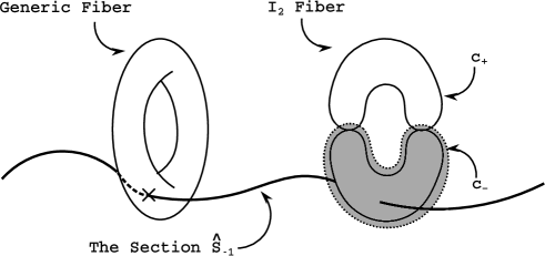
Figure 2: The section ${\hat{S}}_{-1}$. ${\hat{S}}_{-1}$ intersects a generic fiber at a point while is resolved into the $c_{-}$ component at the $I_{2}$ loci.

A quick way to compute the intersection numbers between the homology class ${\hat{S}}_{-1}$ of the section $-{\hat{s}}$ and the fibral curves $c^{I}_{-}$ is the following. Since $c^{I}_{+}$ and $c^{I}_{-}$ intersect at two points,

$${\hat{S}}_{-1}\cdot c^{I}_{+}=2\,,$$ (79)

as ${\hat{S}}_{-1}$ is resolved into $c^{I}_{-}$ at locus $I$. Meanwhile, ${\hat{S}}_{-1}$, being a homology class of the section satisfies

$${\hat{S}}_{-1}\cdot f=1$$ (80)

for the fiber class $f$. Using the fact that

$$f=c^{I}_{-}+c^{I}_{+}$$ (81)

for each $I=1,\cdots,108$, we find that

$${\hat{S}}_{-1}\cdot c^{I}_{-}=-1\,,$$ (82)

which indeed confirms (69).

5.1.2 $m=2$

Let us consider the section given by

$$2{\hat{s}}~{}:~{}[x,y,z]=\left[{\hat{f}}_{12}^{2}-8f_{6}f_{9}^{2},-{\hat{f}}_{12}^{3}+12f_{6}{\hat{f}}_{12}f_{9}-8f_{9}^{4},2f_{9}\right]$$ (83)

in projective coordinates. Again, plugging in the locus of this section

$$x=\left({{\hat{f}}_{12}\over 2f_{9}}\right)^{2}-2f_{6},\quad y=-\left({{\hat{f}}_{12}\over 2f_{9}}\right)^{3}+3f_{6}\left({{\hat{f}}_{12}\over 2f_{9}}\right)^{2}-f_{9}$$ (84)

— in the chart $z=1$ — to equation (70) we find that the matrix $M$ is given by

$$M=\begin{pmatrix}\left({{\hat{f}}_{12}\over 2f_{9}}\right)^{2}-3f_{6}~{}&~{}-\left({{\hat{f}}_{12}\over 2f_{9}}\right)\left\{\left({{\hat{f}}_{12}\over 2f_{9}}\right)^{2}-3f_{6}\right\}\\ -\left({{\hat{f}}_{12}\over 2f_{9}}\right)^{3}+3f_{6}\left({{\hat{f}}_{12}\over 2f_{9}}\right)-2f_{9}~{}&~{}-\left({{\hat{f}}_{12}\over 2f_{9}}\right)\left\{-\left({{\hat{f}}_{12}\over 2f_{9}}\right)^{3}+3f_{6}\left({{\hat{f}}_{12}\over 2f_{9}}\right)-2f_{9}\right\}\\ \end{pmatrix}\,.$$ (85)

Therefore the projective coordinates of the ${\mathbb{{P}}}^{1}$ are given by

$$V:T={\hat{f}}_{12}:2f_{9}$$ (86)

for points of the section above non-degenerate loci on the base.

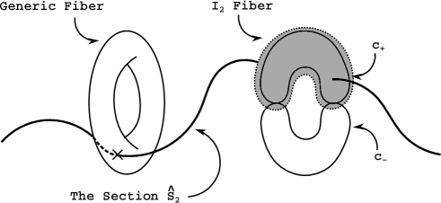
Figure 3: The section ${\hat{S}}_{2}$. ${\hat{S}}_{2}$ intersects a generic fiber at a point while is resolved into the $c_{+}$ component at the $I_{2}$ loci.

At the loci where the fiber becomes degenerate ($f_{9}={\hat{f}}_{12}=0$), the section is not well-defined as all the projective coordinates in (83) become zero. Therefore one must resolve the section at these loci to treat them correctly in the blown-up manifold. This can be done globally by introducing the ${\mathbb{{P}}}^{1}$ coordinates $(P,Q)$ along the section such that

$$f_{9}P-{\hat{f}}_{12}Q=0\quad\Leftrightarrow\quad p={\hat{f}}_{12}/f_{9}\,.$$ (87)

We note that this resolution of the section does not introduce any new divisor in the ambient space. Rather, it attaches curves to the section within the resolved ambient space to produce a “closure” of the section.

As a result, the section $2{\hat{s}}$ is resolved into

$$v=-p,\quad x=4p^{2}-2f_{6}$$ (88)

at the $I_{2}$ loci. This behavior is depicted in figure 3. For each locus $I=1,\cdots,108$, this is precisely the curve $c^{I}_{+}$ by (75). Since $c^{I}_{+}$ intersects the curve $c^{I}_{-}$ at exactly two points, and since the section ${\hat{S}}_{2}$ is resolved into $c^{I}_{+}$ at each $I$,

$${\hat{S}}_{2}\cdot c^{I}_{-}=2$$ (89)

for the fibral curves. This result is consistent with (69).

5.2 $\mathcal{T}_{n}$, $0\leq n\leq 6$

In this section, we study the Calabi-Yau threefolds ${\hat{X}}_{n}$ that yield the theories $\mathcal{T}_{n}$ with $n=0,\cdots,6$. These are six-dimensional $T=0$ supergravity theories with gauge group $U(1)$ and $b=2(n+3)$. Recall that the matter content of $\mathcal{T}_{n}$ is given by $4(n+3)(9-n)$ hypermultiplets with charge $1$ and $n(n+3)$ hypermultiplets with charge $2$. We first derive the Weierstrass models $X_{n}$ using a general construction explained in detail in appendix B. We first check that these manifolds indeed yield $\mathcal{T}_{n}$ indirectly by field theory arguments. We then explicitly verify that the F-theory compactification upon ${\hat{X}}_{n}$ results in $\mathcal{T}_{n}$ by studying the Mordell-Weil generator and its intersection numbers with fibral rational curves.

In appendix B it is shown that a Weierstrass model of an elliptic fibration over field $K$ with Mordell-Weil group of rank one is of the form

$$y^{2}=x^{3}+(c_{1}c_{3}-b^{2}c_{0}-{c_{2}^{2}\over 3})xz^{4}+\left(c_{0}c_{3}^{2}-{1\over 3}c_{1}c_{2}c_{3}+{2\over 27}c_{2}^{3}-{2\over 3}b^{2}c_{0}c_{2}+{b^{2}c_{1}^{2}\over 4}\right)z^{6}$$ (90)

with the Mordell-Weil generator

$$[x,y,z]=[c_{3}^{2}-{2\over 3}b^{2}c_{2},-c_{3}^{3}+b^{2}c_{2}c_{3}-{1\over 2}b^{4}c_{1},b]\,.$$ (91)

Here $c_{i}$ and $b$ are elements of $K$.

There is a straightforward way of utilizing the equation (90) to obtain a class of Weierstrass models of Calabi-Yau threefolds fibered over ${\mathbb{{P}}}^{2}$ with Mordell-Weil rank-one. It is to set

$$c_{3}=f_{3+n},\quad c_{2}=3f_{6},\quad c_{1}=2f_{9-n},\quad c_{0}=f_{12-2n},\quad b=b_{n}$$ (92)

where $f$ and $b$ are polynomials of the base ${\mathbb{{P}}}^{2}$ coordinates whose subscripts denote their degree. The proportionality constants are designated for aesthetic reasons. Under these assignments the Weierstrass form (90) becomes

$$\begin{split}X_{n}~{}:\quad y^{2}&=x^{3}+(2f_{3+n}f_{9-n}-3f_{6}^{2}-b_{n}^{2}f_{12-2n})xz^{4}\\ &+(2f_{6}^{3}-2f_{3+n}f_{6}f_{9-n}+f_{3+n}^{2}f_{12-2n}-2b_{n}^{2}f_{6}f_{12-2n}+{b_{n}^{2}f_{9-n}^{2}})z^{6}\,.\end{split}$$ (93)

The Mordell-Weil generator of the fibration is given by

$${\hat{s}}~{}:~{}[x,y,z]=[f_{3+n}^{2}-2b_{n}^{2}f_{6},-f_{3+n}^{3}+3b_{n}^{2}f_{6}f_{3+n}-b_{n}^{4}f_{9-n},b_{n}]$$ (94)

in mutually relatively prime projective coordinates. Upon compactifying F-theory on these manifolds, one obtains $T=0$ theories with gauge group $U(1)$. From the form of the Mordell-Weil generator, it follows that the anomaly coefficient of the $U(1)$ theory is

$$b=2(n+3)$$ (95)

as explained in section 3.2.

We claim that for each $n$, the low-energy theory obtained by compactifying F-theory on $X_{n}$ is $\mathcal{T}_{n}$. For the rest of this section, we verify this claim by using field theory arguments (section 5.2.1) and by direct computation of intersection numbers in the resolution of $X_{n}$ (section 5.2.2).

We note that the ansatz (93) is valid only for $0\leq n\leq 6$ by the explicit form of the Weierstrass model — since there is polynomial of degree $f_{12-2n}$, $n$ cannot exceed $6$. There is an obvious extension of this ansatz allowing $f_{12-2n}$ to vanish identically if $n>6$, but as we observe in appendix C the Weierstrass model acquires an additional unintended $SU(2)$ gauge factor in the extended ansatz.

5.2.1 Field Theory

A quick way of deriving the low-energy theory of $X_{n}$ is by Higgsing. As commented at the end of appendix B, upon tuning $b_{n}\rightarrow 0$, $X_{n}$ becomes

$$\begin{split}y^{2}=x^{3}+(2f_{3+n}f_{9-n}-3f_{6}^{2})xz^{4}+(2f_{6}^{3}-2f_{3+n}f_{6}f_{9-n}+f_{3+n}^{2}f_{12-2n})z^{6}\,.\end{split}$$ (96)

The discriminant locus of this model is given by

$$f_{3+n}^{2}\left\{36f_{6}^{2}\left(3f_{6}f_{12-2n}\!-\!f_{9-n}^{2}\right)\!+\!f_{3+n}\left(32f_{9-n}^{3}\!-\!108f_{6}f_{9-n}f_{12-n}\!+\!27f_{3+n}f_{12-2n}^{2}\right)\right\}$$ (97)

This theory is an $SU(2)$ theory that has an enhanced gauge group over $f_{3+n}=0$. We have un-Higgsed the $U(1)$ theory to an $SU(2)$ theory by tuning the hypermultiplets by $b_{n}\rightarrow 0$.

Let us examine the properties of the $SU(2)$ model. The anomaly coefficient of the $SU(2)$ group is $(n+3)$, and the $SU(2)$ locus in the base has genus $(n+2)(n+1)/2$. Therefore there are $(n+2)(n+1)/2$ adjoint hypermultiplets in the low-energy spectrum of the $SU(2)$ theory. From the discriminant locus (97) one finds that there are $2(n+3)(9-n)$ fundamental hypermultiplets localized at the loci

$$f_{3+n}=0,\quad 3f_{6}f_{12-2n}-f_{9-n}^{2}=0$$ (98)

in the base, where the $I_{2}$ fiber enhances to an $I_{3}$ fiber. We note that there are not any additional matter localized at

$$f_{3+n}=0,\quad f_{6}=0$$ (99)

as the fiber reduces to a type $III$ fiber at these loci. The mixed/gauge anomaly equations are satisfied for this theory:

$$\mathcal{G}=SU(2)~{}:\quad 2(n+3)(9-n)\times{\tiny\yng(1)}+{(n+2)(n+1)\over 2}\times({\rm Adj}),\qquad b_{SU(2)}=(n+3)\,.$$ (100)

The $U(1)$ theory given by the manifold $X_{n}$ (93) with Mordell-Weil rank-one can be obtained by Higgsing the $SU(2)$ theory in a particular way. There are $J\equiv(n+2)(n+1)/2$ adjoint fields in the $SU(2)$ theory. Turning on these fields ($\Phi_{1},\Phi_{2},\cdots,\Phi_{J}$) to a generic value will completely break the gauge symmetry while turning them on such that

$$\Phi_{1}=c_{1}\sigma_{3},~{}\Phi_{2}=c_{2}\sigma_{3},~{}\cdots,~{}\Phi_{J}=c_{J}\sigma_{3}\,,$$ (101)

breaks the theory to a $U(1)$ theory. The $J=(n+2)(n+1)/2$ parameters $c_{1},\cdots,c_{J}$ are encoded in the $(n+2)(n+1)/2$ coefficients of the polynomial $b_{n}$.

The $U(1)$ theory obtained by Higgsing the adjoint hypermultiplets in this way has $4(n+3)(9-n)$ charge $1$ hypermultiplets coming from the fundamental fields and $n(n+3)$ charge $2$ hypermultiplets coming from the adjoint fields. Its anomaly coefficient is twice of that of the $SU(2)$ theory, as the normalized coroot matrix of $SU(2)$ is $(2)$, i.e.,

$$b=2b_{SU(2)}=2(n+3)\,,$$ (102)

which is consistent with (95). This is precisely the theory $\mathcal{T}_{n}$, as claimed.

5.2.2 Direct Computation

${\mathbb{{C}}}^{*}$	$a$	$b$	$c$	$x$	$y$	$z$
1	$1$	$1$	$1$	$0$	$0$	$-3$
2	$0$	$0$	$0$	$2$	$3$	$1$

Table 2: The toric data of the ambient space of manifold $X_{n}$. $a,b$ and $c$ are the ${\mathbb{{P}}}^{2}$ coordinates, while $x,y$ and $z$ are the fiber coordinates.

Let us verify that $X_{n}$ yields $\mathcal{T}_{n}$ directly from the geometry. We proceed by first resolving $X_{n}$ to a smooth threefold ${\hat{X}}_{n}$. We then work out the resolution of the section (94) under this map and compute its intersection numbers with the fibral rational curves, thereby confirming the charges of the hypermultiplets of the theory.

Let us begin by noting that the Weierstrass model (93),

$$\begin{split}X_{n}~{}:\quad y^{2}&=x^{3}+(2f_{3+n}f_{9-n}-3f_{6}^{2}-b_{n}^{2}f_{12-2n})xz^{4}\\ &+(2f_{6}^{3}-2f_{3+n}f_{6}f_{9-n}+f_{3+n}^{2}f_{12-2n}-2b_{n}^{2}f_{6}f_{12-2n}+{b_{n}^{2}f_{9-n}^{2}})z^{6}\,,\end{split}$$

is a hypersurface of a toric variety whose coordinates and ${\mathbb{{C}}}^{*}$ actions are summarized in table 2 (describing a $\mathbb{P}^{(1,2,3)}$-bundle over $\mathbb{P}^{2}$). The smooth threefold ${\hat{X}}_{n}$ birationally equivalent to $X_{n}$ is given by a hypersurface of a toric variety $T_{n}$ whose data can be summarized by table 3 (describing a bundle over $\mathbb{P}^{2}$ whose fiber is $\operatorname{Bl}_{[0,1,0]}\mathbb{P}^{(1,1,2)}$ — see appendix B).

The birational map between $X_{n}$ and ${\hat{X}}_{n}$ is given by a slight modification of equation (160). Let us examine this map in detail. A useful way of describing the map is to identify ${\mathbb{{C}}}^{*}$ actions of the two toric ambient spaces. We identify ${\mathbb{{C}}}^{*}_{1}$/${\mathbb{{C}}}^{*}_{2}$ of table 2 with ${\mathbb{{C}}}^{*}_{1^{\prime}}$/${\mathbb{{C}}}^{*}_{2^{\prime}}$ of table 3 respectively. Then the birational map (160) can be described in terms of ${\mathbb{{C}}}^{*}_{3^{\prime}}$ invariant coordinates. Defining the ${\mathbb{{C}}}^{*}_{3^{\prime}}$ invariant coordinates of ${\hat{X}}_{n}$ as

$$u:=U,\quad v:=V/T,\quad w:=W/T\,,$$ (103)

the birational map is given by a reparametrized version of (160):

$$\begin{split}x&=f_{3+n}uv+f_{6}u^{2}+b_{n}w\\ y&=b_{n}f_{3+n}uv^{2}+3b_{n}f_{6}u^{2}v+{b_{n}f_{9-n}}u^{3}+f_{3+n}uw+b_{n}^{2}vw\\ z&=u\end{split}$$ (104)

The inverse map is given by

$$\begin{split}v&={b_{n}(y-f_{9-n}b_{n}z^{3})-f_{3+n}(x-f_{6}z^{2})z\over b_{n}^{2}(x+2f_{6}z^{2})-f_{3+n}^{2}z^{2}}\\ w&={-f_{3+n}(y-f_{9-n}b_{n}z^{3})z+b_{n}(x+2f_{6}z^{2})(x-f_{6}z^{2})\over b_{n}^{2}(x+2f_{6}z^{2})-f_{3+n}^{2}z^{2}}\\ u&=z\end{split}$$ (105)

Under this birational map, $X_{n}$ is mapped to

$${\hat{X}}_{n}~{}:\quad TW^{2}-b_{n}WV^{2}=U\left(f_{3+n}V^{3}+3f_{6}TUV^{2}+2f_{9-n}T^{2}U^{2}V+f_{12-2n}T^{3}U^{3}\right)\,,$$ (106)

which is a generic hypersurface in the toric variety $T_{n}$ when $n\leq 6$.

${\mathbb{{C}}}^{*}$	$a$	$b$	$c$	$T$	$U$	$V$	$W$
$1^{\prime}$	$1$	$1$	$1$	$n$	$-3$	$0$	$0$
$2^{\prime}$	$0$	$0$	$0$	$0$	$1$	$1$	$2$
$3^{\prime}$	$0$	$0$	$0$	$1$	$0$	$1$	$1$

Table 3: The toric data of the ambient space $T_{n}$ of manifold ${\hat{X}}_{n}$. $a,b$ and $c$ are the ${\mathbb{{P}}}^{2}$ coordinates. $T,U,V$ and $W$ are the fiber coordinates.

All the fibral rational curves of ${\hat{X}}_{n}$ are isolated, as there are no fibral divisors. These rational curves are components of $I_{2}$ fibers. The fiber degenerates to $I_{2}$ fibers at codimension-two loci above the base in ${\hat{X}}_{n}$. There are two different types of $I_{2}$ loci — charge-two loci and charge-one loci, where isolated rational curves that contribute hypermultiplets of charge-two and one to the six-dimensional spectrum are localized, respectively. There are $n(n+3)$ charge-two loci and $4(n+3)(9-n)$ charge-one loci, as we expect from the preceding discussions.

Let us examine the charge-two loci. From the defining equation (106) it is easy to see that the fiber degenerates at the $n(n+3)$ codimension-two loci in the base

$$b_{n}=0,\quad f_{3+n}=0\,.$$ (107)

At these points, (106) becomes

$$TW^{2}=3f_{6}TU^{2}V^{2}+2f_{9-n}T^{2}U^{3}V+f_{12-2n}T^{3}U^{4}\,.$$ (108)

The two rational curves that consist the $I_{2}$ fiber are

$$\begin{split}\chi^{\iota}_{+}~{}&:\quad T=0\\ \chi^{\iota}_{-}~{}&:\quad W^{2}=3f_{6}U^{2}V^{2}+2f_{9-n}TU^{3}V+f_{12-2n}T^{2}U^{4}\end{split}$$ (109)

at each point indexed by $\iota=1,\cdots,n(n+3)$. We call these loci “charge-two loci,” as the fibral rational curves $\chi_{-}$ sitting above these points contribute hypermultiplets of charge $2$ under the $U(1)$. We can see that the degenerate fiber is indeed an $I_{2}$ fiber as the two curves $\chi^{\iota}_{+}$ and $\chi^{\iota}_{-}$ meet at the two points

$${W\over UV}=\pm\sqrt{3f_{6}}\,.$$ (110)

To verify that $\chi_{-}$ are the fibral curves blown down by the map (104), we can plug in $b_{n}=0,f_{3+n}=0$ to this formula to see that

$$x=f_{6}u^{2},\quad y=0,\quad z=u$$ (111)

when $T\neq 0$. These are exactly the projective coordinates of the singular point of $X_{n}$ at the charge-two locus $b_{n}=0,f_{3+n}=0$, as the Weierstrass model reduces to

$$y^{2} =(x+2f_{6}z^{2})(x-f_{6}z^{2})^{2}$$ (112)

at these points.

Let us verify that the intersection numbers between the Mordell-Weil generator

$${\hat{s}}~{}:~{}[x,y,z]=[f_{3+n}^{2}-2b_{n}^{2}f_{6},-f_{3+n}^{3}+3b_{n}^{2}f_{6}f_{3+n}-b_{n}^{4}f_{9-n},b_{n}]\,,$$ (113)

and the isolated rational curves $\chi^{\iota}_{-}$ at the charge-two loci are indeed given by

$$\sigma({\hat{s}})\cdot\chi^{\iota}_{-}={\hat{S}}\cdot\chi^{\iota}_{-}=2\,.$$ (114)

Plugging in the Weierstrass coordinates of the section (113) into the map (105), we find that the section maps to the point

$$T=0,\quad{W\over UV}=-{f_{3+n}\over b_{n}}$$ (115)

above generic points in the base. The section, however, is not well-defined at the charge-two loci (107). As in section 5.1.2, we resolve these points on the section, i.e., we let

$$b_{n}P-f_{3+n}Q=0\,,$$ (116)

where $(P,Q)$ parametrizes a ${\mathbb{{P}}}^{1}$. By this resolution, the section ${\hat{s}}$ is resolved to the curve $\chi^{\iota}_{+}$ at the charge-two loci. Therefore, the section ${\hat{s}}$ intersects the curves $\chi^{\iota}_{-}$ at two points.

The $I_{2}$ fibers other than the charge-two fibers can be found in the following way. Using the ${\mathbb{{C}}}^{*}_{3^{\prime}}$ invariant coordinates, the equation for ${\hat{X}}_{n}$ can be written in the form

$$(w-{b_{n}\over 2}v^{2})^{2}={1\over 4}b_{n}^{2}v^{4}+f_{3+n}v^{3}+3f_{6}v^{2}+2f_{9-n}v+f_{12-2n}\,,$$ (117)

where we have set $u=1$. The $I_{2}$ loci other than the charge-two loci are the codimension-two points in the base where the right-hand-side of this equation factors into

$$({1\over 2}b_{n}v^{2}+{f_{3+n}\over b_{n}}v+{3b_{n}^{2}f_{6}-f_{3+n}^{2}\over b_{n}^{3}})^{2}\,.$$ (118)

These are the charge-one loci. By equating (117) and (118) we find that the charge-one loci are given by the points that satisfy

$$\begin{split}f_{3+n}^{3}-3f_{6}f_{3+n}b_{n}^{2}+b_{n}^{4}f_{9-n}&=0\\ f_{3+n}^{4}-6f_{6}f_{3+n}^{2}b_{n}^{2}+9f_{6}^{2}b_{n}^{4}-f_{12-2n}b_{n}^{6}&=0\end{split}$$ (119)

that are not charge-two loci. For a generic ${\hat{X}}_{n}$, neither $b_{n}$ nor $f_{3+n}$ vanishes at a charge-one locus.

Near the charge-one loci, the resolution (160) and the section (113) exhibit the same behavior as in $\mathcal{T}_{0}$, which we have extensively studied in section 5.1. To verify this behavior it proves useful to define

$$p_{3}\equiv{f_{3+n}/b_{n}}\,.$$ (120)

The Weierstrass model $X_{n}$ can be written as

$$y^{2}-g_{9}^{2}=(x-g_{6})(x^{2}+g_{6}x+g_{12})$$ (121)

for

$$\begin{split}g_{6}=p_{3}^{2}-2f_{6},\quad g_{9}=-p_{3}^{3}+3f_{6}p_{3}-b_{n}f_{9-n},\\ g_{12}=p_{3}^{4}-4f_{6}p_{3}^{2}+2b_{n}f_{9-n}p_{3}+f_{6}^{2}-b_{n}^{2}f_{12-2n}\,,\end{split}$$ (122)

where we have set $z=1$. The Mordell-Weil generator (113) is given by

$${\hat{s}}~{}:~{}[x,y,z]=[g_{6},g_{9},1]\,.$$ (123)

Also, the birational map (105) can be re-written in the form

$$\begin{split}b_{n}v&={y+g_{9}\over x-g_{6}}-p_{3}\\ b_{n}w&=-p_{3}b_{n}v+(x+{g_{6}\over 2}-{p_{3}^{2}\over 2})\end{split}$$ (124)

The charge-one loci (119) are the loci at which

$$\begin{split}g_{9}&=-p_{3}^{3}+3f_{6}p_{3}-b_{n}f_{9-n}=0\\ \hat{g}_{12}&\equiv g_{12}+2g_{6}^{2}=3p_{3}^{4}-12f_{6}p_{3}^{2}+2b_{n}f_{9-n}p_{3}+9f_{6}^{2}-b_{n}^{2}f_{12-2n}=0\end{split}$$ (125)

From the fact that $b_{n}$, $f_{n+3}$ and $p_{3}$ are all well-defined and non-zero at the charge-one loci, it is clear that the analysis of section 5.1 can be readily applied to understanding these points.

The singular fibers of $X_{n}$ located above these points are resolved into $I_{2}$ fibers that consist of two rational curves:

$$c^{I}_{\pm}~{}:~{}w-{b_{n}\over 2}v^{2}=\pm\left({1\over 2}b_{n}v^{2}+p_{3}v+{p_{3}^{2}-3g_{6}\over 2b_{n}}\right)\,.$$ (126)

We have used $I$ to index the charge-one loci. Using the full set of projective coordinates, these curves can be written as

$$c^{I}_{\pm}~{}:~{}TW-{b_{n}\over 2}V^{2}=\pm\left({1\over 2}b_{n}V^{2}+p_{3}TUV+{p_{3}^{2}-3g_{6}\over 2b_{n}}T^{2}U^{2}\right)\,.$$ (127)

The zero-section,

$$U=0,\quad{TW\over V^{2}}=b_{n}\,,$$ (128)

intersects the curve $c^{I}_{+}$ at a single point, while the Mordell-Weil generator (115),

$$T=0,\quad{W\over UV}=-p_{3}\,,$$ (129)

intersects $c^{I}_{-}$ also at a single point. Therefore the isolated rational curve at the charge-one locus $I$ is $c^{I}_{-}$ and its intersection number with the Mordell-Weil generator is indeed given by

$$\sigma({\hat{s}})\cdot c^{I}_{-}={\hat{S}}\cdot c^{I}_{-}=1\,.$$ (130)

It is clear that ${\hat{s}}$ is a Mordell-Weil generator, as there exist curves of unit intersection number with ${\hat{S}}$.

Let us now show that there are $4(n+3)(9-n)$ charge-one loci. To count the number of charge-one loci, one must count the number of points that satisfy (119), but at which $b_{n}\neq 0$ and $f_{n+3}\neq 0$. To show that there are $4(n+3)(9-n)$ such points, it is enough to show this in the case when

$$b_{n}=\epsilon B_{n}$$ (131)

for $\epsilon$ that is in a small neighborhood of $0$. To do so, let us first rewrite (119) as

$$\begin{split}p_{3}^{3}-3f_{6}p_{3}+b_{n}f_{9-n}&=0\\ p_{3}^{4}-6f_{6}p_{3}^{2}+9f_{6}^{2}-b_{n}^{2}f_{12-2n}&=0\\ \end{split}$$ (132)

and view these equations as polynomial equations with respect to $p_{3}$. These two equations can have a unique common root

$$p_{3}={b_{n}f_{9-n}f_{12-2n}\over 3f_{6}f_{12-2n}-f_{9-n}^{2}}$$ (133)

only when

$$(f_{9-n}^{2}-3f_{6}f_{12-2n})^{2}=b_{n}^{2}f_{12-2n}^{3}\,.$$ (134)

When $|\epsilon|<<1$,

$$f_{n+3}={f_{9-n}(3f_{6}f_{12-2n}-f_{9-n}^{2})\over f_{12-2n}^{2}}=\mathcal{O}(\epsilon)\,.$$ (135)

At small enough $\epsilon$, for each point satisfying the two equations (133) and (134), there exists a nearby point satisfying

$$f_{n+3}=0\,,$$ (136)

along with (134). Therefore when $\epsilon$ lies in a small enough neighborhood of $0$, there are $(n+3)(36-4n)$ charge-one loci. We note when the theory is enhanced to an $SU(2)$ theory by taking $\epsilon\rightarrow 0$, the charge-one loci merge in pairs to the codimension-two points defined by

$$f_{n+3}=0,\quad f_{9-n}^{2}-3f_{6}f_{12-2n}=0\,.$$ (137)

These are precisely the points above which the fundamental hypermultiplets of the enhanced $SU(2)$ sit.

We have shown that there are two types of isolated fibral rational curves in ${\hat{X}}_{n}$ — those localized above charge-two loci and and those localized above charge-one loci in the base. The $n(n+3)$ charge-two rational curves intersect the Mordell-Weil generator ${\hat{S}}$ twice while the $4(n+3)(9-n)$ charge-one rational curves intersect ${\hat{S}}$ once. We have summarized these facts in figure 4.

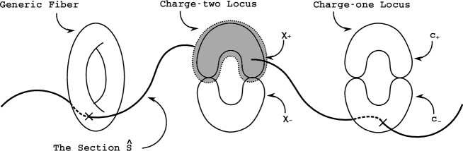
Figure 4: The intersection between the section ${\hat{S}}$ and fiber components in ${\hat{X}}_{n}$. ${\hat{S}}$ intersects a generic fiber at a point. There are $n(n+3)$ charge-two loci and $4(n+3)(9-n)$ charge-one loci in the base above which the fiber degenerates into an $I_{2}$ fiber. The fibral curves $\chi_{-}^{\iota}$ localized above the charge-two loci intersect the section ${\hat{S}}$ twice, while the fibral curves $c_{-}^{I}$ at the charge-one loci intersect ${\hat{S}}$ once.

6 Questions and Future Directions

There are a host of questions regarding the Mordell-Weil group of elliptically fibered Calabi-Yau threefolds that we have not pursued in this note. We conclude by listing some interesting questions — in what we believe is to be the order of increasing difficultly — that could hopefully be addressed in the not-so-distant future.

Models with $n=7,8$
Out of the nine $T=0$, $U(1)$ theories with hypermultiplets of charges $\leq 2$ allowed by anomaly equations, we have only constructed F-theory models for seven. Although we have not been able to construct the two theories — which we have denoted $\mathcal{T}_{7}$ and $\mathcal{T}_{8}$ in section 4 — we expect these theories to be embeddable in F-theory.

This expectation comes from the fact that the $U(1)$ theories $\mathcal{T}_{n}$ can be obtained by Higgsing the adjoint hypermultiplets of an $SU(2)$ theory with $2(n+3)(9-n)$ fundamental hypermultiplets and ${(n+2)(n+1)/2}$ adjoint hypermultiplets. Let us denote the $SU(2)$ theories by $\mathcal{T}_{n}^{\prime}$. The non-abelian theory $\mathcal{T}_{n}^{\prime}$ has anomaly coefficient $b=10$($b=11$) and $88$($97$) neutral hypermultiplets for $n=7$($n=8$) respectively. We are not aware of any obstruction in embedding these un-Higgsed $SU(2)$ theories into F-theory as they satisfy all the anomaly constraints and also the Kodaira constraint, i.e., $b<18$ for both these models. It is on these grounds that we expect $\mathcal{T}_{7,8}^{\prime}$ — and $\mathcal{T}_{7,8}$, which can be obtained from $\mathcal{T}_{7,8}^{\prime}$ by Higgsing — to be embeddable in F-theory.

We have not, however, been able explicitly construct the threefolds that yield $\mathcal{T}_{7,8}^{\prime}$, let alone $\mathcal{T}_{7,8}$. The difficulty in constructing these theories originates from the fact that the ring of polynomials with two variables is not a Euclidean ring. This implies that the ansätz (93), (96) we have used to construct Weierstrass models for $\mathcal{T}_{n}$, $\mathcal{T}_{n}^{\prime}$ do not necessarily generalize to all possible $n$.

It would be interesting to explicitly construct $\mathcal{T}_{7,8}$/$\mathcal{T}_{7,8}^{\prime}$ or prove that they cannot be engineered as F-theory models. It would be intriguing if $\mathcal{T}_{7}^{\prime}$ or $\mathcal{T}_{8}^{\prime}$ defies expectations and is shown to be un-embeddable in F-theory. This would imply that the Kodaira constraint is not a sharp enough criterion for discerning whether a non-abelian theory can be embedded in F-theory or not.

Models with General Charges
A natural question to ask in light of the results of this note is whether there exist models with more general charges. We have seen in section 5.1 that a rational section can intersect fibral rational curves with an arbitrary intersection number. Therefore it is sensible to expect that there exist six-dimensional supergravity theories with more general charges — charges greater than $2$ — that are embeddable in F-theory.

An efficient strategy of finding F-theory backgrounds with hypermultiplets of charge $\geq 3$ might be to first construct $SU(2)$ theories with hypermultiplets in higher-spin representations in addition to adjoints, and then to obtain the $U(1)$ theories by Higgsing its adjoint hypermultiplets. For example, if there exists an $SU(2)$ theory with a hypermultiplet in the representation $J=3/2$ along with an adjoint ($J=1$,) one can obtain a $U(1)$ theory with hypermultiplets of charge $\pm 3$ by Higgsing the adjoint field. It would be interesting to see if one could find all such $SU(2)$ theories at least in the case when $T=0$. There is reason to be optimistic about this goal, given recent developments on the space of $T=0$ theories such as [11, 61].

A question that follows is whether there exist $U(1)$ models in F-theory that cannot be enhanced to $SU(2)$. We are not aware of any reason to believe that such models do not exist. If such models exist, however, engineering them is expected to be an algebraic challenge for reasons that could be deduced from the way we have constructed elliptic fibrations with Mordell-Weil rank-one in appendix B. Let us present the argument restricting to the case when $T=0$ for sake of simplicity.

It is shown in appendix B that the Mordell-Weil generator of a threefold can be written in the form

$${\hat{s}}~{}:\quad[x,y,z]=[c_{3}^{2}-{2\over 3}b^{2}c_{2},-c_{3}^{3}+b^{2}c_{2}c_{3}-{1\over 2}b^{4}c_{1},b]\,.$$ (138)

in Weierstrass coordinates. If there are enough degrees of freedom in $b$ for it to be tuned to $0$, this model can be enhanced to an $SU(2)$ theory, as described at the end of appendix B. This is indeed the case for all the models we have constructed in this note — in fact, $b$ is an arbitrary polynomial of degree $n$, whose coefficients could all be tuned to zero for the manifolds presented in section 5. Therefore, in order for its low-energy $U(1)$ theory to be “un-enhancable,” an elliptically fibered threefold with Mordell-Weil rank-one must be “rigid,” in the sense that its complex structure must be fixed at a certain point. Such loci in the F-theory moduli space are difficult to find.

It would nevertheless be interesting to identify such models and compare them to what is allowed from anomaly constraints. If the string universality conjecture [7] holds, there should be a correspondence between non-trivial solutions of the $U(1)$ anomaly equations (49), (50) and these special un-enhancable points in the F-theory moduli space. Whether such a correspondence indeed exists remains to be seen.

A Generalized Kodaira Constraint
We return to the question that initiated our study of models with Mordell-Weil rank-one — is there a generalized version of the Kodaira constraint for the abelian sector of six-dimensional F-theory models? In the case of $T=0$ F-theory models with gauge group $U(1)$, we have simplified the question. Recall that these models come from compactifying F-theory on elliptically fibered Calabi-Yau threefolds over ${\mathbb{{P}}}^{2}$ with Mordell-Weil rank-one and no fibral divisors. The Néron-Tate height of a rational section of such a manifold is given by a number. The analogue of the Kodaira condition in this case would be a bound on the Néron-Tate height of the generator of the Mordell-Weil group. From arguments presented in the introduction, such a bound should indeed exist — it would be very interesting to find what that bound is.

In the event that such a bound on the height of the Mordell-Weil generator is attained, it would be interesting to see how it is modified in more general situations. For example, this bound might be modified when there is non-abelian gauge symmetry. Also, when the Mordell-Weil rank is larger than one — i.e., when there are multiple $U(1)$’s — such a bound is expected to generalize to a constraint on the height-pairing matrix of the basis of the Mordell-Weil group. We can further generalize to theories with $T>0$ — i.e., when the base of the elliptic fibration is a general rational surface rather than a ${\mathbb{{P}}}^{2}$ [62, 63, 64]. In this case, the height pairing of rational sections become divisors in the base, rather than numbers. Such bounds, if attained, will play a crucial role in gaining a better understanding of the space of six-dimensional F-theory vacua, and ultimately the space of six-dimensional supergravity theories.

Appendix A Addition of Sections

An elliptic curve over a field may be written in Weierstrass form:

$$\begin{split}y^{2}&=x^{3}+fxz^{4}+gz^{6}\end{split}$$ (139)

as a hypersurface of ${\mathbb{{P}}}[2,3,1]$, where $(x,y,z)$ are its projective coordinates.

Let us define the “zero point” of the elliptic curve to be at $(x,y,z)=(1,1,0)$. Working in the affine chart $z=1$, we can now define the addition “${[+]}$” of two points $p=(a,b)$ and $P=(A,B)$ on an elliptic curve over a field. The symbol “${[+]}$” is used for this algebraic addition to distinguish from addition defined in the homology ring. Note that

$$\begin{split}y^{2}&=x^{3}+fx+g\\ &=(x-a)(x^{2}+ax+c)+b^{2}\\ &=(x-A)(x^{2}+Ax+C)+B^{2}\,.\\ \end{split}$$ (140)

The new point $\mathcal{P}=p{[+]}P=(\mathcal{A},\mathcal{B})$ is obtained by demanding that $(\mathcal{A},-\mathcal{B})$ is the third intersection point of the line that goes through the two points $p$ and $P$. It can easily be shown that

$$\mathcal{P}=\left(\left({B-b\over A-a}\right)^{2}-(a+A),-\left({B-b\over A-a}\right)^{3}+(2a+A)\left({B-b\over A-a}\right)-b\right)\,.$$ (141)

One could also find $\mathcal{P}^{\prime}=P{[+]}P=(\mathcal{A}^{\prime},\mathcal{B}^{\prime})$ by demanding that $(\mathcal{A}^{\prime},-\mathcal{B}^{\prime})$ is the other intersection point of the tangent line of the elliptic curve that goes through $P$. $\mathcal{P}^{\prime}$ is given by

$$\mathcal{P}^{\prime}=\left(\left({C+2A^{2}\over 2B}\right)^{2}-2A,-\left({C+2A^{2}\over 2B}\right)^{3}+3A\left({C+2A^{2}\over 2B}\right)-B\right)\,.$$ (142)

It can be shown that the rational points of the elliptic curve form an abelian group under the group action “${[+]}$” — the action is commutative and associative, and the zero point is the identity element of the action. It is also clear that $a{[+]}b$ is a rational point when $a$ and $b$ are rational points.

Appendix B Elliptic Fibrations with Two Sections

In this appendix, we construct the Weierstrass model for elliptic fibrations with two rational sections over a field $K$. We begin by reviewing how to arrive at a Weierstrass model given the condition that there exists one section. We proceed to obtain the Weierstrass model when there are two sections.

Let us first review how to arrive at the Weierstrass model of an elliptic curve $E$ over a field $K$ with a point $P$, or more generally, over a ring $R$ whose fraction field is $K$. We start with the line bundle $L=\mathcal{O}(P)$ and consider sections: $H^{0}(L)$ has a single section, denoted by $z$. $H^{0}(2L)$ has two sections, one of which is $z^{2}$ and the other of which is new, which we denote $x$. $H^{0}(3L)$ has three sections: $z^{3}$, $xz$, and a new one $y$. $H^{0}(4L)$ has four sections: $z^{4}$, $xz^{2}$, $yz$, and $x^{2}$. $H^{0}(5L)$ has five sections: $z^{5}$, $xz^{3}$, $yz^{2}$, $x^{2}z$, and $xy$. $H^{0}(6L)$ should only have six sections, but we know about seven: $z^{6}$, $xz^{4}$, $yz^{3}$, $x^{2}z^{2}$, $xyz$, $x^{3}$, $y^{2}$. Thus, there must be a relation, and one argues — following Deligne [65] — that the coefficients of $x^{3}$ and $y^{2}$ must be units in the ring $R$ and after an appropriate scaling, we get a Weierstrass equation of the form

$$y^{2}+a_{1}xyz+a_{3}yz^{3}=x^{3}+a_{2}x^{2}z^{2}+a_{4}xz^{4}+a_{6}z^{6}\,.$$ (143)

Since the variables $z$, $x$, and $y$ have weights $1$, $2$, and $3$, this can be regarded as a hypersurface in the weighted projective space $\mathbb{P}^{(1,2,3)}$, which as a toric variety is illustrated in the first row of figure 5. The monomials which occur in equation (143) are indicated as a polytope contained in the monomial lattice $M$, and the toric divisors $D_{x}$, $D_{y}$, and $D_{z}$ are indicated as the generators of the polar polytope in the dual lattice $N$.

 

Figure 5: Toric data for ambient spaces of some elliptic curve embeddings. These are among the 16 reflexive toric surfaces [66] (see also [67]).

Typically the Weierstrass equation is studied in the affine chart $z=1$. If the characteristic of $K$ is not 2 or 3 (which is true in our case), we can complete the square in $y$ and then complete the cube in $x$, resulting in an equation with $a_{1}=a_{2}=a_{3}=0$.

Now let us consider the case with two sections. Suppose that we have an elliptic curve over a field $K$ with two points $P$ and $Q$, coming from two sections of the elliptic fibration. We assume that both points are defined over $K$, but do not assume that they are necessarily distinct. This time we use the line bundle $M=\mathcal{O}(P+Q)$ and again study sections. We first study sections and an embedding in the case of an arbitrary line bundle $M$ of degree $2$, and subsequently specialize to the case of $M=\mathcal{O}(P+Q)$.

Since $H^{0}(M)$ has two sections, we let $u$, $v$ be a basis of this space. Now $H^{0}(2M)$ has four sections: $u^{2}$, $uv$, $v^{2}$, and a new one which we denote by $w$. The space $H^{0}(3M)$ has six sections, all of which are known: $u^{3}$, $u^{2}v$, $uv^{2}$, $v^{3}$, $uw$ and $vw$. Finally, $H^{0}(4M)$ should have eight sections, but we know nine: $u^{4}$, $u^{3}v$, $u^{2}v^{2}$, $uv^{3}$, $v^{4}$, $uvw$, $u^{2}w$, $v^{2}w$, and $w^{2}$. Thus, there must be an equation. It is not hard to argue that the coefficient of $w^{2}$ must be a unit (in order that the solution set be a genus one curve) and that by scaling we can set that coefficient equal to 1:

$$w^{2}+b_{0}u^{2}w+b_{1}uvw+b_{2}v^{2}w=c_{0}u^{4}+c_{1}u^{3}v+c_{2}u^{2}v^{2}+c_{3}uv^{3}+c_{4}v^{4}\,.$$ (144)

Since the variables $u$, $v$, and $w$ have weights $1$, $1$, and $2$, we can regard this as defining a hypersurface in the weighted projective space $\mathbb{P}^{(1,1,2)}$, which as a toric variety is illustrated in the second row of figure 5. Again, the monomials in (144) are shown, as well as the toric divisors $D_{u}$, $D_{v}$, and $D_{w}$.

We can specialize the form of the equation further if we assume that $M=\mathcal{O}(P+Q)$. In this case, we choose $u$ to be a section which vanishes precisely at $P$ and $Q$, and let $v$ be an arbitrary second section which vanishes elsewhere. When we set $u=0$ in (144), we get

$$w^{2}+b_{0}v^{2}w=c_{4}v^{4}$$ (145)

and so the two roots of this equation must correspond to $P$ and $Q$. Since $P$ and $Q$ are defined over the ground field $K$, this equation must factor; then, shifting $w$ by an appropriate multiple of $v$ we can assume that one of the factors is $w$, i.e., that $c_{4}=0$. This leaves us with an equation of the form

$$w^{2}+b_{0}u^{2}w+b_{1}uvw+b_{2}v^{2}w=u(c_{0}u^{3}+c_{1}u^{2}v+c_{2}uv^{2}+c_{3}v^{3})\,.$$ (146)

This is again a general hypersurface in a toric variety. The difference between (144) and (146) is that the monomial $v^{4}$ has been eliminated, as illustrated in the third row of figure 5. The corresponding change to the polar polytope corresponds to blowing up $\mathbb{P}^{(1,1,2)}$ at the point $[0,1,0]$, giving a new exceptional divisor which is denoted by $E_{1}$.

Assuming the characteristic of $K$ is not 2, we can further shift $w$ by a multiple of $u$ to also assume that $b_{0}=b_{1}=0$. Let us simplify notation and denote $b_{2}$ simply by $b$. Thus we obtain an equation of the form

$$w^{2}+bv^{2}w=u(c_{0}u^{3}+c_{1}u^{2}v+c_{2}uv^{2}+c_{3}v^{3})\,,$$ (147)

in which the point $P$ has $[u,v,w]=[0,1,0]$ and the point $Q$ has $[u,v,w]=[0,1,-b]$.

Let us find the Weierstrass form of this fibration (147) corresponding to the section $P$. For this purpose, we need to find sections of $H^{0}(kM-kQ)$, that is, sections of $H^{0}(kM)$ which vanish $k$ times along $Q$. The first of these is easy: the section $u$ vanishes along Q, and so in our construction of a Weierstrass model we take

$$z:=u\,.$$ (148)

Now we need sections of $H^{0}(2M)$, that is, linear combinations of $w$ and a quadratic in $v$ and $u$. One such section is $u^{2}$; to find another, we set

$$w=\alpha v^{2}+\beta uv+\gamma u^{2}$$ (149)

and substitute in the equation:

$$\begin{split}&u(c_{0}u^{3}+c_{1}u^{2}v+c_{2}uv^{2}+c_{3}v^{3})\\ &=w(w+bv^{2})=(\alpha v^{2}+\beta uv+\gamma u^{2})((b+\alpha)v^{2}+\beta uv+\gamma u^{2})\,.\end{split}$$ (150)

To get $Q$ at $u=0$ we need $\alpha=-b$. Thus, our equation becomes

$$u(c_{0}u^{3}+c_{1}u^{2}v+c_{2}uv^{2}+c_{3}v^{3})=(-bv^{2}+\beta uv+\gamma u^{2})(\beta uv+\gamma u^{2})\,.$$ (151)

We need a double zero at $u=0$, which requires $c_{3}=-b\beta$. Thus, we should take $\beta=-c_{3}/b$ and hence

$$w=-bv^{2}-(c_{3}/b)uv+\gamma u^{2}\,.$$ (152)

We can omit the $u^{2}$ term since it is another solution.

More generally, we can clear denominators, and take the second element of our Weierstrass form to be

$$x:=b^{2}v^{2}+bw+c_{3}uv\,.$$ (153)

Next, we need sections of $H^{0}(3M)$ vanishing three times at $Q$. Two of these are $u^{3}$ and $u(b^{2}v^{2}+bw+c_{3}uv)$, so we seek a section of the form $vw=\alpha v^{3}+\beta uv^{2}+\gamma u^{2}v$ omitting terms of the form $uw$ and $u^{3}$ since they are taken care of by other sections. In this case, we substitute into the equation as follows:

$$\begin{split}&uv^{2}(c_{0}u^{3}+c_{1}u^{2}v+c_{2}uv^{2}+c_{3}v^{3})\\ &=(vw)(vw+bv^{3})=(\alpha v^{3}+\beta uv^{2}+\gamma u^{2}v)((b+\alpha)v^{3}+\beta uv^{2}+\gamma u^{2}v)\,.\end{split}$$ (154)

As in the previous case, we need $\alpha=-b$ to guarantee that at $u=0$ we are getting $Q$, which leads to an equation

$$uv^{2}(c_{0}u^{3}+c_{1}u^{2}v+c_{2}uv^{2}+c_{3}v^{3})=(-bv^{3}+\beta uv^{2}+\gamma u^{2}v)(\beta uv^{2}+\gamma u^{2}v)\,.$$ (155)

To get a triple zero at $u=0$, we then require

$$\begin{split}c_{2}&=-b\gamma+\beta^{2}\\ c_{3}&=-b\beta\end{split}$$ (156)

which is solved by

$$\begin{split}\alpha&=-b\\ \beta&=-c_{3}/b\\ \gamma&=-c_{2}/b+c_{3}^{2}/b^{3}\,.\end{split}$$ (157)

Thus, to complete our mapping to a Weierstrass model, we mostly clear denominators and use

$$y:=b^{2}vw+b^{3}v^{3}+bc_{3}uv^{2}+(bc_{2}-{c_{3}^{2}\over b})u^{2}v\,.$$ (158)

The Weierstrass equation in these coordinates is given by

$$y^{2}-x^{3}+\frac{2c_{3}}{b}xyz+{c^{2}_{3}-b^{2}c_{2}\over b^{2}}x^{2}z^{2}+bc_{1}yz^{3}+b^{2}c_{0}xz^{4}+c_{0}(b^{2}c_{2}-c^{2}_{3})z^{6}=0\,.$$ (159)

By the reparametrization

$$\begin{split}{\tilde{x}}&=x+{c_{2}\over 3}z^{2}=b^{2}v^{2}+c_{3}uv+{c_{2}\over 3}u^{2}+bw\\ {\tilde{y}}&=y+{c_{3}\over b}xz+{bc_{1}\over 2}z^{3}=b^{3}v^{3}+2bc_{3}uv^{2}+bc_{2}u^{2}v+{bc_{1}\over 2}u^{3}+c_{3}uw+b^{2}vw\\ z&=u\end{split}$$ (160)

we arrive at the standard Weierstrass form:

$${\tilde{y}}^{2}={\tilde{x}}^{3}+(c_{1}c_{3}-b^{2}c_{0}-{c_{2}^{2}\over 3}){\tilde{x}}z^{4}+\left(c_{0}c_{3}^{2}-{1\over 3}c_{1}c_{2}c_{3}+{2\over 27}c_{2}^{3}-{2\over 3}b^{2}c_{0}c_{2}+{b^{2}c_{1}^{2}\over 4}\right)z^{6}\,.$$ (161)

To find the section $Q$ explicitly, we return to sections of $H^{0}(2M)$, this time looking for a section which vanishes three times at $Q$. In our setup above, we have used $w=\alpha v^{2}+\beta uv+\gamma u^{2}$, and found the condition to vanish to order-two at $Q$. Now we need to vanish to order-three, which gives one additional equation:

$$c_{2}=-b\gamma+\beta^{2}\,.$$ (162)

The solution, after normalization, is

$$b^{2}v^{2}+bw+c_{3}uv+(c_{2}-{c^{2}_{3}\over b^{2}})u^{2}=x+(c_{2}-{c^{2}_{3}\over b^{2}})z^{2}\,.$$ (163)

In other words, the $x$-coordinate of $Q$ is $((c_{3}/b)^{2}-c_{2})z^{2}$. Substituting the corresponding ${\tilde{x}}$ value into equation (161), we can solve for ${\tilde{y}}$. The section can in fact be located at

$$[{\tilde{x}},{\tilde{y}},z]=[c_{3}^{2}-{2\over 3}b^{2}c_{2},-c_{3}^{3}+b^{2}c_{2}c_{3}-{1\over 2}b^{4}c_{1},b]\,.$$ (164)

The transition from an extra section to an enhanced $SU(2)$ is obtained when $b$ becomes identically zero, which means that the sections $P$ and $Q$ are exactly the same. It can be seen that the fiber at $c_{3}=0$ has Kodaira type $I_{2}$, i.e., it is an $SU(2)$ fiber.

Appendix C A Degenerate Limit

Suppose we have an elliptic fibration with two sections for which the coefficients $b_{0}$ and $c_{0}$ in (146) vanish identically, or equivalently, after completing the square, the coefficent $c_{0}$ in (147) vanishes identically. In this case, the ambient toric variety changes dramatically, as indicated in the fourth row of figure 5.

First, setting $c_{0}=0$ in (146) corresponds to a second blowup of $\mathbb{P}^{(1,1,2)}$ at $[1,0,0]$, giving an exceptional divisor $E_{2}$. Then, setting $b_{0}=0$ in (146) corresponds to a third blowup with corresponding exceptional divisor $E_{3}$. At this stage, however, the divisors $D_{v}$ and $E_{2}$ have intersection number zero with the canonical divisor of the toric surface, so they are blown down in the anti-canonical model of the toric variety.

More significant than the change in the toric variety, however, is the behavior of the discriminant locus of the Weierstrass equation. The Weierstrass equation for this family is determined by setting $c_{0}=0$ in (161) (since we have already completed the square), yielding

$${\tilde{y}}^{2}={\tilde{x}}^{3}+(c_{1}c_{3}-{c_{2}^{2}\over 3}){\tilde{x}}z^{4}+\left(-{1\over 3}c_{1}c_{2}c_{3}+{2\over 27}c_{2}^{3}+{b^{2}c_{1}^{2}\over 4}\right)z^{6}\,.$$ (165)

It is straightforward to compute the discriminant of (165) and we find:

$$\frac{1}{16}c_{1}^{2}\left(27b^{4}c_{1}^{2}+16b^{2}c_{2}^{3}-72b^{2}c_{1}c_{2}c_{3}-16c_{2}^{2}c_{3}^{2}+64c_{1}c_{3}^{3}\right)\,.$$ (166)

Note that when $c_{1}=0$, the coefficients of ${\tilde{x}}z^{4}$ and $z^{6}$ do not necessarily vanish.

The interpretation of the factor of $c_{1}^{2}$ in this discriminant is as follows. Whenever we have an elliptic fibration with two sections of this form — with the coefficients being sections of appropriate line bundles over the base — the fibration will have fibers of Kodaira type $I_{2}$ along the locus $c_{1}=0$. In particular, in F-theory there will be a locus with enhanced $SU(2)$ gauge symmetry.

The candidate models for $\mathcal{T}_{7}$ and $\mathcal{T}_{8}$ discussed in section 5.2 are precisely of this form — these manifolds were constructed by setting $f_{12-2n}=0$ in the ansatz (93). We now see that those constructions do not have simply a $U(1)$ gauge symmetry, but have an additional $SU(2)$ gauge symmetry, which is not what is desired.

Note that there is one exception to this conclusion, that is, when $c_{1}$ itself is nowhere-vanishing. In the body of the paper, we have considered a situation in which $c_{1}$ is a polynomial of degree $(9-n)$ on $\mathbb{P}^{2}$. If $n=9$, $c_{1}$ does not vanish and indeed the “$\mathcal{T}_{9}$ theory” agrees with the $\mathcal{T}_{0}$ theory but with the “wrong” choice of generating section.

References

- [1] T. W. Grimm, T. Weigand, “On Abelian Gauge Symmetries and Proton Decay in Global F-theory GUTs,” Phys. Rev. D82, 086009 (2010). [arXiv:1006.0226 [hep-th]].
- [2] E. Dudas, E. Palti, “On hypercharge flux and exotics in F-theory GUTs,” JHEP 1009, 013 (2010). [arXiv:1007.1297 [hep-ph]].
- [3] J. Marsano, “Hypercharge Flux, Exotics, and Anomaly Cancellation in F-theory GUTs,” Phys. Rev. Lett. 106, 081601 (2011). [arXiv:1011.2212 [hep-th]].
- [4] M. J. Dolan, J. Marsano, N. Saulina, S. Schafer-Nameki, “F-theory GUTs with U(1) Symmetries: Generalities and Survey,” Phys. Rev. D84, 066008 (2011). [arXiv:1102.0290 [hep-th]].
- [5] J. Marsano, N. Saulina, S. Schafer-Nameki, “On G-flux, M5 instantons, and U(1)s in F-theory,” [arXiv:1107.1718 [hep-th]].
- [6] T. W. Grimm, M. Kerstan, E. Palti, T. Weigand, “Massive Abelian Gauge Symmetries and Fluxes in F-theory,” [arXiv:1107.3842 [hep-th]].
- [7] V. Kumar and W. Taylor, “String Universality in Six Dimensions,” arXiv:0906.0987 [hep-th].
- [8] V. Kumar and W. Taylor, “A Bound on 6D N=1 supergravities,” JHEP 0912, 050 (2009) [arXiv:0910.1586 [hep-th]].
- [9] V. Kumar, D. R. Morrison and W. Taylor, “Mapping 6D N = 1 supergravities to F-theory,” JHEP 1002, 099 (2010) [arXiv:0911.3393 [hep-th]].
- [10] V. Kumar, D. R. Morrison and W. Taylor, “Global aspects of the space of 6D N = 1 supergravities,” JHEP 1011, 118 (2010) [arXiv:1008.1062 [hep-th]].
- [11] V. Kumar, D. S. Park and W. Taylor, “6D supergravity without tensor multiplets,” JHEP 1104, 080 (2011) [arXiv:1011.0726 [hep-th]].
- [12] D. S. Park and W. Taylor, “Constraints on 6D Supergravity Theories with Abelian Gauge Symmetry,” JHEP 1201, 141 (2012) [arXiv:1110.5916 [hep-th]].
- [13] D. R. Morrison and C. Vafa, “Compactifications of F theory on Calabi-Yau threefolds. 1,” Nucl. Phys. B 473, 74 (1996) [hep-th/9602114].
- [14] D. R. Morrison and C. Vafa, “Compactifications of F theory on Calabi-Yau threefolds. 2.,” Nucl. Phys. B 476, 437 (1996) [hep-th/9603161].
- [15] D. S. Park, “Anomaly Equations and Intersection Theory,” JHEP 1201, 093 (2012) [arXiv:1111.2351 [hep-th]].
- [16] M. R. Gaberdiel and B. Zwiebach, “Exceptional groups from open strings,” Nucl. Phys. B 518, 151 (1998) [hep-th/9709013].
- [17] O. DeWolfe and B. Zwiebach, “String junctions for arbitrary Lie algebra representations,” Nucl. Phys. B 541, 509 (1999) [hep-th/9804210].
- [18] M. Fukae, Y. Yamada and S. -K. Yang, “Mordell-Weil lattice via string junctions,” Nucl. Phys. B 572, 71 (2000) [hep-th/9909122].
- [19] Z. Guralnik, “String junctions and nonsimply connected gauge groups,” JHEP 0107, 002 (2001) [hep-th/0102031].
- [20] P. S. Aspinwall and D. R. Morrison, “Nonsimply connected gauge groups and rational points on elliptic curves,” JHEP 9807, 012 (1998) [hep-th/9805206].
- [21] R. Donagi, P. Gao and M. B. Schulz, “Abelian Fibrations, String Junctions, and Flux/Geometry Duality,” JHEP 0904, 119 (2009) [arXiv:0810.5195 [hep-th]].
- [22] K. Hulek and R. Kloosterman, “Calculating the Mordell-Weil rank of elliptic threefolds and the cohomology of singular hypersurfaces,” Ann. Inst. Fourier (Grenoble) 61, no. 3, 1133-1179 (2011) [arXiv:0806.2025v3 [math.AG]].
- [23] J. I. Cogolludo-Agustin and A. Libgober, “Mordell-Weil groups of elliptic threefolds and the Alexander module of plane curves,” [arXiv:1008.2018v2 [math.AG]].
- [24] R. Kloosterman, “Cuspidal plane curves, syzygies and a bound on the MW-rank,” [arXiv:1107.2043v3 [math.AG]].
- [25] J. I. Cogolludo-Agustin and R. Kloosterman, “Mordell-Weil groups and Zariski triples,” [arXiv:1111.5703v1 [math.AG]].
- [26] K. Kodaira, “On Compact Analytic Surfaces II,” Annals of Math. 77, 563-626 (1963).
- [27] Y. Kawamata, “Kodaira dimension of certain algebraic fiber spaces,” J. Fac. Sci. Univ. Tokyo Sec. IA 30, 1-24 (1983).
- [28] T. Fujita, “Zariski decomposition and canonical rings of elliptic threefolds,” J. Math. Soc. Japan 38, 19-37 (1986).
- [29] N. Nakayama, “On Weierstrass models,” Algebraic Geometry and Commutative Algebra vol. II, Kinokuniya, Tokyo, 405-431 (1988).
- [30] A. Grassi, “On minimal models of elliptic threefolds,” Math. Ann. 290, 287-301 (1991).
- [31] A. Grassi, “Log contractions and equidimensional models of elliptic threefolds,” J. Algebraic Geom. 4, 255-276 (1995) [arXiv:alg-geom/9305003].
- [32] M. Gross, “A finiteness theorem for elliptic Calabi-Yau threefolds,” Duke Math. J. 74 271-299 (1994) [arXiv:alg-geom/9305002].
- [33] M. B. Green, J. H. Schwarz, “Anomaly Cancellation in Supersymmetric D=10 Gauge Theory and Superstring Theory,” Phys. Lett. B149, 117-122 (1984).
- [34] M. B. Green, J. H. Schwarz, P. C. West, “Anomaly Free Chiral Theories in Six-Dimensions,” Nucl. Phys. B254, 327-348 (1985).
- [35] A. Sagnotti, “A Note on the Green-Schwarz mechanism in open string theories,” Phys. Lett. B 294, 196 (1992) [arXiv:hep-th/9210127].
- [36] V. Sadov, “Generalized Green-Schwarz mechanism in F theory,” Phys. Lett. B388, 45-50 (1996). [hep-th/9606008].
- [37] F. Riccioni, “Abelian vector multiplets in six-dimensional supergravity,” Phys. Lett. B 474, 79 (2000) [arXiv:hep-th/9910246].
- [38] F. Riccioni, “All couplings of minimal six-dimensional supergravity,” Nucl. Phys. B 605, 245 (2001) [arXiv:hep-th/0101074].
- [39] S. L. Adler, “Axial vector vertex in spinor electrodynamics,” Phys. Rev. 177, 2426 (1969).
- [40] J. S. Bell and R. Jackiw, “A PCAC puzzle: pi0 gamma gamma in the sigma model,” Nuovo Cim. A 60, 47 (1969).
- [41] L. Alvarez-Gaume and E. Witten, “Gravitational Anomalies,” Nucl. Phys. B 234, 269 (1984).
- [42] J. Erler, “Anomaly Cancellation In Six-Dimensions,” J. Math. Phys. 35, 1819 (1994) [arXiv:hep-th/9304104].
- [43] G. Honecker, “Massive U(1)s and heterotic five-branes on K3,” Nucl. Phys. B748, 126-148 (2006) [hep-th/0602101].
- [44] M. Bershadsky, K. A. Intriligator, S. Kachru, D. R. Morrison, V. Sadov, C. Vafa, “Geometric singularities and enhanced gauge symmetries,” Nucl. Phys. B481, 215-252 (1996). [hep-th/9605200].
- [45] T. Shioda, “Mordell-Weil lattices and Galois representation. I,” Proc. Japan Acad. 65A, 268-271 (1989).
- [46] T. Shioda, “On the Mordell-Weil Lattices,” Comment. Math. Univ. St. Pauli 39, 211-240 (1990).
- [47] F. Bonetti and T. W. Grimm, “Six-dimensional (1,0) effective action of F-theory via M-theory on Calabi-Yau threefolds,” JHEP 1205, 019 (2012) [arXiv:1112.1082 [hep-th]].
- [48] J. H. Silverman, “The arithmetic of elliptic curves,” Dordrecht: Springer (2009) xx+513 pp. (Graduate Texts in Mathematics, 106)
- [49] R. Wazir, “Arithmetic on elliptic threefolds,” Compos. Math. 140, 567-580 (2004) math/0112259 [math.NT].
- [50] D. R. Morrison and W. Taylor, “Matter and singularities,” JHEP 1201, 022 (2012) [arXiv:1106.3563 [hep-th]].
- [51] S. Katz, D. R. Morrison, S. Schafer-Nameki and J. Sully, “Tate’s algorithm and F-theory,” JHEP 1108, 094 (2011) [arXiv:1106.3854 [hep-th]].
- [52] M. Esole and S. -T. Yau, “Small resolutions of SU(5)-models in F-theory,” arXiv:1107.0733 [hep-th].
- [53] S. Krause, C. Mayrhofer and T. Weigand, “ flux, chiral matter and singularity resolution in F-theory compactifications,” Nucl. Phys. B 858, 1 (2012) [arXiv:1109.3454 [hep-th]].
- [54] T. W. Grimm and H. Hayashi, “F-theory fluxes, Chirality and Chern-Simons theories,” JHEP 1203, 027 (2012) [arXiv:1111.1232 [hep-th]].
- [55] J. Polchinski, “Monopoles, duality, and string theory,” Int. J. Mod. Phys. A19S1, 145-156 (2004). [hep-th/0304042].
- [56] T. Banks, N. Seiberg, “Symmetries and Strings in Field Theory and Gravity,” Phys. Rev. D83, 084019 (2011). [arXiv:1011.5120 [hep-th]].
- [57] S. Hellerman, E. Sharpe, “Sums over topological sectors and quantization of Fayet-Iliopoulos parameters,” [arXiv:1012.5999 [hep-th]].
- [58] N. Seiberg, W. Taylor, “Charge Lattices and Consistency of 6D Supergravity,” [arXiv:1103.0019 [hep-th]].
- [59] A. Klemm, P. Mayr and C. Vafa, “BPS states of exceptional noncritical strings,” In *La Londe les Maures 1996, Advanced quantum field theory* 177-194 [hep-th/9607139].
- [60] J. Louis, J. Sonnenschein, S. Theisen and S. Yankielowicz, “Nonperturbative properties of heterotic string vacua compactified on K3 x t**2,” Nucl. Phys. B 480, 185 (1996) [hep-th/9606049].
- [61] V. Braun, “Toric Elliptic Fibrations and F-Theory Compactifications,” arXiv:1110.4883 [hep-th].
- [62] D. R. Morrison and W. Taylor, “Classifying bases for 6D F-theory models,” arXiv:1201.1943 [hep-th].
- [63] D. R. Morrison and W. Taylor, “Toric bases for 6D F-theory models,” arXiv:1204.0283 [hep-th].
- [64] W. Taylor, “On the Hodge structure of elliptically fibered Calabi-Yau threefolds,” arXiv:1205.0952 [hep-th].
- [65] P. Deligne, “Courbes elliptiques: formulaire d’après J. Tate,” Modular functions of one variable, IV (Proc. Internat. Summer School, Univ. Antwerp, Antwerp, 1972), Lecture Notes in Math., vol. 476, Springer, Berlin, 1975, pp. 53-73.
- [66] M. Kreuzer and H. Skarke, “On the classification of reflexive polyhedra,” Comm. Math. Phys. 185 495-508 (1997) [arXiv:hep-th/9512204].
- [67] A. Grassi and V. Perduca, “Weierstrass models of elliptic toric K3 hypersurfaces and symplectic cuts,” [arXiv:1201.0930 [math.AG]].
- [68] G. Aldazabal, A. Font, L. E. Ibanez, and A. M. Uranga, “New branches of string compactifications and their F-theory duals,” Nucl. Phys. B 492 119-151 (1997) [arXiv:hep-th/9607121].
- [69] P. Berglund, A. Klemm, P. Mayr, and S. Theisen, “On type IIB vacua with varying coupling constant,” Nucl. Phys. B 558 178-204 (1999) [arXiv:hep-th/9805189].
- [70] P. Aluffi and M. Esole, “New orientifold weak coupling limits in F-theory,” JHEP 1002 020 (2010) [arXiv:0908.1572 [hep-th]].