Turbulent Coronal Heating Mechanisms: Coupling of
Dynamics and Thermodynamics

Abstract

Context. Photospheric motions shuffle the footpoints of the strong axial magnetic field that threads coronal loops giving rise to turbulent nonlinear dynamics characterized by the continuous formation and dissipation of field-aligned current sheets where energy is deposited at small-scales and the heating occurs. Previous studies show that current sheets thickness is orders of magnitude smaller than current state of the art observational resolution ($\sim 700\,km$).

Aims. In order to understand coronal heating and interpret correctly observations it is crucial to study the thermodynamics of such a system where energy is deposited at unresolved small-scales.

Methods. Fully compressible three-dimensional magnetohydrodynamic simulations are carried out to understand the thermodynamics of coronal heating in the magnetically confined solar corona.

Results. We show that temperature is highly structured at scales below observational resolution and nonhomogeneously distributed so that only a fraction of the coronal mass and volume gets heated at each time.

Conclusions. This is a multi-thermal system where hotter and cooler plasma strands are found one next to the other also at sub-resolution scales and exhibit a temporal dynamics.

1 Introduction

Magnetohydrodynamic (MHD) turbulence has long been implicated as a key process in coronal heating (Einaudi et al., 1996) as well as fast and slow solar wind acceleration. Numerical simulations have been crucial in investigating the role of MHD turbulence.

To tackle the turbulence problem correctly with direct numerical simulations, it is necessary to resolve enough spatial scales to obtain an energy containing range, an inertial range, and a dissipation range. Because of storage needs, the more the complexity of the problem is reduced, the more spatial scales are obtainable. Hence most previous research in this area has been restricted to dynamical effects, e.g., reduced MHD (RMHD) (Strauss, 1976) and cold plasma models. This reduces the size of the problem considerably. For example, for RMHD the dynamics of the system are determined by two variables: a stream function and a magnetic potential function (Rappazzo et al., 2007). For the cold plasma model it is customary to evolve three velocity field components and three magnetic field components, neglecting the pressure term (thus not correcting for the solenoidality of the velocity field) so that six variables are used (Dahlburg et al., 2009).

In all these approximations all thermodynamical aspects are lost, i.e., there is no information on the connection between the dynamics of the system, responsible for the heating mechanism, and the temperature and density behavior. In particular energy lost through Ohmic and viscous diffusion is simply lost from the system and the thermodynamic physics involved with thermal conduction and optically thin radiation is neglected.

This lack of information prevents a complete reproduction of the energy cycle: photospheric motions shuffle magnetic field-lines footpoints injecting energy into the Corona and triggering non-linear dynamics that form small-scales, organized in current sheets (Parker, 1972),where energy is then transformed into thermal (and kinetic and perturbed magnetic) energy by means of magnetic reconnection. Heat is then conducted from the high temperature corona back toward the low temperature photosphere where it is lost via optically thin radiation, but at the same time causing chromospheric evaporation.

Thermodynamics are typically studied with 1D hydrodynamic models (Reale, 2010) that study either the equilibrium condition of a heated loop, or the time-dependent evaporative and possible condensation flows. However they introduce an ad hoc heating function to mimic the energy deposition and neglect the cross-field dynamics (including field-lines reconnection). It is therefore crucial to use the computationally more demanding three-dimensional compressible MHD (with eight variables), including an energy equation with thermal conduction and the energy sink provided by optically thin radiation.

RMHD turbulence simulations (Rappazzo et al., 2007, 2008) have shown that in the planes orthogonal to the DC magnetic field the length of current sheets is of the order of the photospheric convective cells scale (i.e., $\sim 1,000\,km$), while their width is much smaller and limited only by numerical resolution. In order to understand the thermodynamics of such system in this letter we carry out simulations that resolve the scales below the convection scale. The boundary conditions used in this paper do not allow evaporative flows to develop along the heated loops, our focus here is on the relationship of turbulent current sheet dissipation and the forming coronal temperature structure.

Our new compressible code HYPERION has allowed us to make a start at examining the fully compressible, three-dimensional Parker coronal heating model. HYPERION is a parallelized Fourier collocation finite difference code with third-order Runge-Kutta time discretization that solves the compressible MHD equations with vertical thermal conduction and radiation included. The results provided by this new compressible code preserve the spatial intermittency of the kinetic and magnetic energies seen in earlier RMHD simulations, but also provide new information about the evolution of the internal energy, i.e., we can now determine how the coronal plasma heats up and radiates energy as a consequence of photospheric convection of magnetic footpoints (Dahlburg et al., 2010).

In Section 2 we describe the governing equations, the boundary and initial conditions, and the numerical method. In Section 3 we detail our numerical results. Section 4 contains a discussion of these results and some ideas about future directions of this research.

2 Formulation of the problem

2.1 Governing equations

We model the solar corona as a compressible, dissipative magnetofluid. The equations which govern such a system, written here in dimensionless form, are:

$${{\partial n}\over{\partial t}}\ = \ -\nabla\cdot(n{\bf v}),$$ (1)

$${{\partial n{\bf v}}\over{\partial t}}\ = \ -\nabla\cdot({n\bf vv})-{\beta}\nabla p+{\bf J}\times{\bf B}+{1\over S_{v}}\nabla\cdot{\bf\zeta},$$ (2)

$${{\partial T}\over{\partial t}}\ = \ -{\bf v}\cdot\nabla T-(\gamma-1)(\nabla\cdot{\bf v})T+\frac{1}{n}\big{\{}\frac{1}{Pr\,S_{v}}\frac{\partial}{\partial z}(T^{\frac{5}{2}}\frac{\partial T}{\partial z})$$ (3)

$$\ +{(\gamma-1)\over\beta}[{1\over S_{v}}\zeta_{ij}e_{ij}+{1\over S}(\nabla\times{\bf B})^{2}-{1\over P_{rad}S_{v}}n^{2}\Lambda(T)$$

$$\ +{\beta\over(\gamma-1)}nC_{N}]\big{\}},$$

$${{\partial{\bf B}}\over{\partial t}}\ = \ \nabla\times{\bf v}\times{\bf B}+\frac{1}{S}\nabla\times\nabla\times{\bf B},$$ (4)

with the solenoidality condition $\nabla\cdot{\bf B}=0$. The system is closed by the equation of state

$$p=nT.$$ (5)

The non-dimensional variables are defined in the following way: $n({\bf x},t)$ is the numerical density, ${\bf v}({\bf x},t)=(u,v,w)$ is the flow velocity, $p({\bf x},t)$ is the thermal pressure, ${\bf B}({\bf x},t)=(B_{x},B_{y},B_{z})$ is the magnetic induction field, ${\bf J}=\nabla\times{\bf B}$ is the electric current density, $T({\bf x},t)$ is the plasma temperature, $\zeta_{ij}=\mu(\partial_{j}v_{i}+\partial_{i}v_{j})-\lambda\nabla\cdot{\bf v}\delta_{ij}$ is the viscous stress tensor, $e_{ij}=(\partial_{j}v_{i}+\partial_{i}v_{j})$ is the strain tensor, and $\gamma$ is the adiabatic ratio. To render the equations dimensionless we have used $n_{0}$, the photospheric numerical density, $V_{A}$, the vertical Alfvén speed at the photospheric boundaries, $L_{0}$, the orthogonal box length (= $L_{x}$ = $L_{y}$) and $T_{0}$, the photospheric temperature. Therefore time ($t$) is measured in units of Alfvén cross time ($\tau_{A}=L_{0}/V_{A}$).

The function $\Lambda(T)$ that describes the temperature dependence of the radiation is taken following Hildner (1974), normalized with its value at the base temperature $T_{0}=10000\,K$. The term $C_{N}$ denotes a Newton thermal term which is enforced at low temperatures to take care of the delicate chromospheric and transition region energy balance (Dorch & Nordlund, 1999). We use $C_{N}=0.1\leavevmode\nobreak\ [T_{i}(z)-T(z)]e^{-2(z+0.5\leavevmode\nobreak\ L_{z})}$ at the lower wall and $C_{N}=0.1\leavevmode\nobreak\ [T_{i}(z)-T(z)]e^{-2(0.5\leavevmode\nobreak\ L_{z}-z)}$ at the upper wall, where $T_{i}(z)$ is the initial temperature profile.

The important dimensionless numbers are: $S_{v}=\rho_{0}V_{A}L_{0}/\mu\equiv$ viscous Lundquist number, $S=\mu_{0}V_{A}L_{0}/\eta\equiv$ Lundquist number, $\beta=\mu_{0}p_{0}/B_{0}^{2}\equiv$ pressure ratio at the wall, $Pr=C_{v}\mu/\kappa T_{0}^{5/2}\equiv$ Prandtl number, and $P_{rad}$, the radiative Prandtl number ${\mu/\tau_{A}^{2}n_{0}^{2}\Lambda(T_{0})}$, determines the strength of the radiation. $C_{v}$ is the specific heat at constant volume. The term ”$\kappa$” denotes the thermal conductivity. The magnetic resistivity $(\eta)$ and shear viscosity $(\mu)$ are assumed to be constant and uniform, and Stokes relationship is assumed so the bulk viscosity $\lambda=(2/3)\mu$.

2.2 Initial and Boundary Conditions

We solve the governing equations in a Cartesian box of dimensions $1\times 1\times L_{z}$, where $L_{z}$ is the loop aspect ratio ($0\leq x,y\leq 1,\ -L_{z}/2\leq z\leq L_{z}/2$), threaded by a DC magnetic field $B_{0}$ in the $z$-direction. The system has periodic boundary conditions in $x$ and $y$, and line-tied boundary conditions at the top and bottom $z$-plates where the vertical flows vanish ($v_{z}=0$) and the forcing velocity in the $x$-$y$ plane is imposed as in previous studies (Hendrix et al., 1996; Einaudi et al., 1996; Einaudi & Velli, 1999) evolving the stream function

$$\psi(x,y,t)=f_{1}\sin^{2}\left(\frac{\pi t}{2t^{*}}\right)+f_{2}\sin^{2}\left(\frac{\pi t}{2t^{*}}+\frac{\pi}{2}\right),$$ (6)

where $f_{i}(x,y)=\sum_{n,m}a_{nm}^{i}sin(k_{n}x+k_{m}y+\zeta_{nm}^{i})$, and $\mathbf{v}=\nabla\psi\times\mathbf{\hat{e}}_{z}$. All wave-numbers with $3\leq(k_{n}^{2}+k_{m}^{2})^{1/2}\leq 4$ are excited, so that the typical length-scale of the eddies is $\sim 1/4$. As the typical convective cell size is $\sim 1,000\,km$ and we use $L_{z}=5$ this implies that our computational box in conventional units spans $4,000^{2}\times 20,000\,km^{3}$. Every $t^{*}$, the coefficients $a_{nm}^{i}$ and the $\zeta_{nm}^{i}$ are randomly changed alternatively for eddies 1 and 2. The magnetic field is expressed as $\mathbf{B}=B_{0}\mathbf{\hat{e}}_{z}+\mathbf{b}$, where $\mathbf{A}$ is the vector potential associated with the fluctuating magnetic field $\mathbf{b}=\nabla\times\mathbf{A}$. At the top and bottom $z$-plates $B_{z}$, n and T are kept constant at their initial values $B_{0}$, $n_{0}$ and $T_{0}$, while the magnetic vector potential is convected by the resulting flows.

In what follows we have assumed the normalizing quantities to be: $n_{0}=10^{17}\,m^{-3}$, $T_{0}=10^{4}\,K$, $B_{0}=10^{-2}$ tesla, and $L_{0}=4\times 10^{6}\,m$. It follows that the values of the various parameters appearing in the equations are: $\beta=1.7\times 10^{-4}$, $v_{A}=6.9\times 10^{5}\,m/s$, $\tau_{A}=5.8\,s$, $S=2.7\times 10^{9}$, $S_{v}=2.09\times 10^{9}$, $Pr=1.52\times 10^{-2}$, $P_{rad}=3.35\times 10^{-6}$, $\kappa\times T_{0}^{5/2}=0.18\,Wm^{-1}K^{-1}$, $\ln\Lambda=10$.

The normalized time scale of the forcing, $t^{*}$, is set to 51.7 to represent the 5 minutes typical photospheric convection time scale. The normalized photospheric velocity is $V_{0}=1.45\times 10^{-3}$, corresponding to $10^{3}\,m/s$.

We impose as initial conditions a temperature profile with a base temperature $T_{0}=10^{4}\,K$ and a top temperature $8\times 10^{5}\,K$ with the following z-dependence for the nondimensional temperature $T_{i}(z)=1+79\cos(\pi z/L_{z})$, while the numerical density is given as $n_{i}(z)=1/T_{i}(z)$. This choice allows us to neglect the gravitational effects since for most of the loop the temperature remains high enough to make the gravitational length-scale bigger than $L_{z}$ at all times.

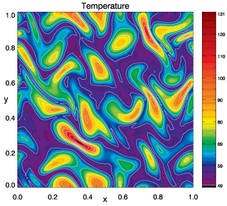
Figure 1: Temperature contours at $t=300$ in the midplane ($z=0)$. Maximum (130) and minimum (49) temperatures correspond to $1.3$ million and $490$ thousand degrees Kelvin in conventional units. Distances are normalized by $L_{0}=4\times 10^{6}\leavevmode\nobreak\ m$.

3 Results

With previous definitions equation (4) can be replaced by the magnetic vector potential equation:

$${\partial{\bf A}\over\partial t}={\bf v}\times(B_{0}\,\mathbf{\hat{e}}_{z}+\nabla\times{\bf A})+{1\over S}\leavevmode\nobreak\ \nabla\times\nabla\times{\bf A}$$ (7)

We solve numerically the equations (1)-(3) and (7) together with equation (5). Space is discretized in $x$ and $y$ with a Fourier collocation scheme (Dahlburg & Picone, 1989) with isotropic truncation dealiasing. Spatial derivatives are calculated in Fourier space, and nonlinear product terms are advanced in configuration space. A second-order central difference technique (Dahlburg, Montgomery & Zang, 1986) is used for the discretization in $z$. A time-step splitting scheme is employed. The code has been parallelized using MPI. A domain decomposition is employed in which the computational box is sliced up into $x$–$y$ planes along the $z$ direction.

We present the results obtained running the code with $S=S_{v}=4\times 10^{4}$ with a resolution of $128^{3}$. In order to keep the efficiency of the radiative and conductive terms in the energy equation as in the real corona, we have rescaled $Pr$ and $P_{rad}$ accordingly with the choice of $S_{v}$, i.e., $Pr=793.39$ and $P_{rad}=0.175$. This choice is due to the result found in the RMHD model (Rappazzo et al., 2008) that turbulent dissipative processes are independent of viscosity and resistivity when an inertial range is well resolved.

The system starts out in a ground state, threaded by a guide magnetic field: the interior of the channel has zero perturbed velocity and magnetic fields. The footpoints of the magnetic field are subjected to convection at the $z$ boundaries with initial number density and temperature profiles assigned as described above. The behavior of the volume averaged quantities, such as kinetic and fluctuating magnetic energies and resistive and viscous dissipation show a temporal behavior similar to the previous RMHD results obtained by Rappazzo et al. (2007, 2008, 2010).

The fluctuating magnetic and kinetic energies ($e_{v}={1\over 2}\langle n{\mathbf{v}}^{2}\rangle$ and $e_{b}={1\over 2}\langle{\mathbf{b}}^{2}\rangle$), as shown in previous RMHD model, and the total internal energy ($U=\langle nT\rangle{\beta/(\gamma-1)}$), not obtainable in the RMHD case exhibit an intermittent behavior. After the system is driven by photospheric motions for more than $100$ Alfvén times a statistically stationary state is attained and all quantities fluctuate around their steady values.

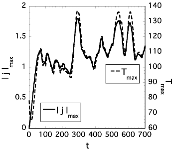
Figure 2: Maximum temperature ($T_{max}$) and maximum electric current $|{\bf j}|_{max}$ as functions of time.

We have verified that the dynamics of this problem are well represented by RMHD. We define the volume-averaged velocity $\theta_{v}$ and magnetic $\theta_{b}$ anisotropy angles as in Shebalin et al. (1983). For isotropic turbulence, $\theta_{v}$ and $\theta_{b}$ would equal $45^{\circ}$. For fully anisotropic turbulence, $\theta_{v}$ and $\theta_{b}$ would equal $90^{\circ}$, implying that their spectra would be normal to $B_{0}\,\mathbf{\hat{e}}_{z}$. We find that, after $t=100$, $\theta_{b}$ is always bigger than $87^{\circ}$, while the velocity field fluctuations are found to be slightly more anisotropic than those in the magnetic field, $88^{\circ}<\theta_{v}<89^{\circ}$, indicating that the turbulence in the present system is highly anisotropic, i.e., the turbulence is strongly confined to planes orthogonal to the guide magnetic field. Moreover we have verified that the dynamics is almost incompressible.

The important new result of this letter refers to the thermodynamical behavior of the system resulting from the self-consistent heating due to the magnetic field-line tangling induced by photospheric motions, once the cooling effects of conduction and radiation are taken into account. The fact that the total internal energy, as mentioned above, fluctuates around a steady value means that the self-consistent heating mechanism due to photospheric motions is efficient enough to sustain a hot corona once the system has reacted to photospheric motion. Such a reaction leads to the formation of small scales where energy can be efficiently dissipated. The small scales, corresponding to the presence of current sheets, are not uniformly distributed in the system, and as a result the temperature is spatially intermittent, as shown in Figure 1, where we show the midplane temperature contours at $t=300$.

Figure 2 shows the time evolution of $T_{max}$ and $|{\bf j}|_{max}$, the maximum temperature and the maximum current density present in the loop at each time respectively. It can be seen that the $T_{max}$ temperature peaks oscillate in time and, after an initial transient, the $T_{max}$ values are well above $T=10^{6}\,K$, higher than the initial peak temperature of $T=8\times 10^{5}\,K$ degrees. An important fact to emphasize is that the peaks in $T_{max}$ roughly coincide with bursts in the maximum electric current. Since currents are organized in sheets elongated along the mean magnetic field and the heating is due to the dissipation of currents we expect the heating not to be homogeneously distributed throughout the loop.

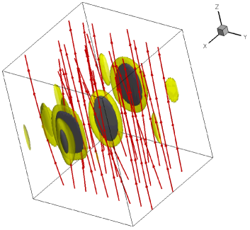
Figure 3: Temperature is organized in quasi-2D pancake-like structures aligned with the magnetic field. The two isosurfaces for $T=10^{6}\,K$ and $T=1.2\times 10^{6}\,K$ at time $t=300$ are shown respectively in yellow and grey (corresponding to $T=100,120$ in nondimensional units). Sample magnetic field-lines are drawn in red. The box has been rescaled to improve visualization.

This expectation is confirmed by Figure 3, where a 3-D snapshot of the isosurfaces of two temperatures ($T=10^{6}$ and $T=1.2\times 10^{6}\,K$) at $t=300$ is presented. The spatial temperature morphology shows that the high temperatures are reached in selected quasi-2D regions elongated along the mean magnetic field where the system dynamics places at each time the current sheets where energy is dissipated. The higher temperatures are found at the center of these structures (up to $1.35\times 10^{6}\,K$ at $t=300$), while farther out the temperature falls off to a background value that in the central z-region averages around $6\times 10^{5}\,K$. Snapshots taken at different times show similar behavior with different high temperatures locations.

4 Conclusions and discussion

In this paper we have presented for the first time the thermodynamic behavior of a system where the conductive and radiative losses are balanced by the heating process due solely to the photospheric motions and the subsequent tangling of magnetic field lines, resolving the scales below convection. While previous compressible simulation (Gudiksen & Nordlund, 2002; Bingert & Peter, 2011) have considered entire active regions resolving at most the convective scale, it is pivotal to resolve smaller scales in order to understand how the plasma is heated and its observational consequences.

A lot of work has been done in the past to show the reaction of a plasma subject to mass flow at its boundaries. It has been shown that the system reacts developing a weak turbulent state, where energy is dissipated in the current sheets resulting from the dynamics induced by the boundary velocity forcing. The results of the present work show that this process leads to a loop where the temperature is spatially highly structured.

A loop is therefore a multi-thermal system, where the temperature peaks around current sheets and exhibits a distribution of temperatures. The characteristics of this distribution (peak, width, background) will vary depending on the parameters of the loop (length, boundary velocity, mean magnetic field).

Temperature and heating are highly nonhomogeneously distributed so that only a fraction of the loop volume exhibits a significant heating at each time. Therefore emission observed in a spectral band origins from the small sub-volume at the corresponding temperature, whose mass is considerably lower that the total loop mass.

Observations currently have a spatial resolution of $\sim 700\,km$ and a temporal resolution of $\sim 30\,s$. These temperature structures are therefore unresolved, and to interpret observations correctly the spatial and temporal intermittency must be taken into account. We intend to present in a following paper how our loop appears once the emission is averaged over the coarser observational resolutions. At those scales the loop might result multithermal or approximately isothermal depending on the loop parameters.

It is very likely that the local thermodynamical equilibrium is lost and that the emission is due to particles accelerated in the current sheets rather than direct transformation of magnetic energy into thermal energy. This is beyond the MHD model.

We have shown that the heating due to photospheric motions is able to balance the losses and that the dynamics induced by the such motions is a multi-scale dynamics where the energy is released in a number of spatial spots which account for the observed emission.

The density stratification in our simulation allows limited evaporation from the z-boundary edges, where density is higher but does not reach typical chromospheric values. In future work we plan to implement characteristic boundary conditions (e.g., Rappazzo et al., 2005) that allow higher density flows through the $z$-boundaries, that can also give rise to condensation and prominences, and study their impact on the thermodynamics.