Exploring criticality in the QCD-like two quark flavour models

Abstract

The critical end-point (CEP) and critical behaviour in its vicinity, has been explored in the two flavour effective chiral models with and without the presence of effective Polyakov loop potential.The tricritical point (TCP) in the massless chiral limit has been located on the phase diagram in the $\mu$ and T plane for the Polyakov loop extended Quark Meson Model (PQM) and pure Quark Meson (QM) model which become effective Quantum-chromodynamics (QCD) like models due to the proper accounting of fermionic vacuum loop contribution in the effective potential.The proximity of the TCP to the QCD critical end-point (CEP) has been quantified in the phase diagram. The critical region around CEP has been obtained in the presence as well as the absence of fermionic vacuum loop contribution in the effective potentials of PQM and QM models. The contours of appropriately normalized constant quark number susceptibility and scalar susceptibility have been plotted around CEP in different model scenarios. These contours determine the shape of critical region and facilitate comparisons in different models such that the influence of fermionic vacuum term and Polyakov loop potential on the critical behavior around CEP can be ascertained in qualitative as well as quantitative terms. Critical exponents resulting from the divergence of quark number susceptibility at the CEP, have been calulated and compared with in different model scenarios. The possible influence of TCP on the critical behavior around CEP, has also been discussed. The temperature variation of $\sigma$ and $\pi$ meson masses at $\mu=0$, $\mu=\mu_{CEP}$ and $\mu>\mu_{CEP}$ has been shown and compared with in different model scenarios and the emerging mass degeneration trend in the $\sigma$ and $\pi$ meson mass variations has been inferred as the chiral symmetry restoration takes place at higher temperatures.

I Introduction

Under the extreme conditions of high temperature and/or density, normal hadronic matter undergoes a phase transition, where the individual hadrons dissolve into their quark and gluon constituents and produce a collective form of matter known as the Quark Gluon Plasma(QGP)Rischke:03 ; Ortmanns:96ea ; Muller ; Svetitsky . Study of the different aspects of this phase transition,is a tough and challenging task because Quantum Chromodynamics(QCD) which is the theory of strong interaction, becomes nonperturbative in the low energy limit. However the QCD vacuum reveals itself through the process of spontaneous chiral symmetry breaking and phenomenon of color confinement.

The QCD Lagrangian is known to have the global $SU_{L+R}(N_{f})\times SU_{L-R}(N_{f})$ symmetry for $N_{f}$ flavours of massless quarks. The formation of a chiral condensate in the low energy hadronic vacuum of QCD, leads to the spontaneous breaking of the axial (A=R-L) part of this symmetry known as the chiral symmetry and one gets $(N_{f}^{2}-1)$ massless Goldstone bosons according to the Goldstone’s theorem. Since quarks are not massless in real life, chiral symmetry of the QCD lagrangian gets explicitly broken and massless modes become pseudo-Goldstone bosons after acquiring mass. Nevertheless, the observed lightness of pions in nature suggests that we have an approximate chiral symmetry for QCD with two falvours of light u and d quarks. In the opposite limit of infinitely heavy quarks, QCD becomes a pure $SU(N_{c})$ gauge theory which remains invariant under the global $Z(N_{c})$ center symmetry of the color gauge group. The Center symmetry which is a symmetry of hadronic vacuum, gets spontaneously broken in the high temperature/density regime of QGP. The expectation value of the Wilson line (Polyakov loop) is related to the free energy of a static color charge. It vanishes in the confining phase as the quark has infinite free energy and becomes finite in the deconfined phase. Hence the Polyakov loop serves as the order parameter of the confinement-deconfinement phase transition Polyakov:78plb . Even though the center symmetry is always broken with the inclusion of dynamical quarks in the system, one can regard the Polyakov loop as an approximate order parameter because it is a good indicator of a rapid crossover in the confinement-deconfinement transition Pisarski:00prd ; Vkt:06 .

Lattice QCD simulations (see e.g. AliKhan:2001ek ; Karsch:02 ; Forcra ; Fodor:03 ; Allton:05 ; Aoki:06 ; Karsch:05 ; Karsch:07ax ; Cheng:06 ; Cheng:08 ; Digal:01 ) give us important information and insights regarding various aspects of the QGP transition, like the restoration of chiral symmetry in QCD, order of the confinement-deconfinement phase transition, richness of the QCD phase structure and phase diagram mapping. Since lattice calculations are technically involved and various issues are not conclusively settled within the lattice community, one resorts to the calculations within the ambit of phenomenological models developed in terms of effective degrees of freedom. These models serve to complement the lattice simulations and give much needed insight about the regions of phase diagram inaccessible to lattice simulations.

Construction and mapping of the phase diagram in the quark chemical potential and temperature plane is the prime challenge before the experimental as well as theoretical QGP community. On the temperature axis, the chiral transition at zero quark chemical potential with almost physical quark masses, has been well established to be a crossover in recent lattice QCD simulationsAoki:06 ; Bazavov . Effective chiral model studiesWilczek predict first order phase transition at lower tempertaures on the chemical potential axis. Thus the existence of a critical end point(CEP) has been suggested in the phase diagram based on model studiesAsaka ; Barducci ; Berges together with the inputs from lattice simulationsForcra ; Fodor:03 ; Allton:05 . The first order transition line starting from the lowest temperarute on the chemical potential axis, terminates at the CEP which is a genuine singularity of the QCD free energy. Here the phase transition turns second order and its criticality belongs to the three dimensional Ising universality class Hatta ; Fujii ; KFuku ; Sour . The precise location of the CEP is highly sensitive to the value of the strange quark mass. Lattice QCD predictions at non zero chemical potential are much more difficult due to the QCD action becoming complex on account of the fermion sign problem Karsch:02 . There is evidence for a CEP at finite $\mu$Forcra ; Fodor:03 from a Taylor expansion of QCD pressure around $\mu=0$, however in another lattice study, finite chemical potential extrapolations provide some limitations and can rule out the existence of a CEP for small $\mu$/T ratiosPhilip . In the chiral limit of zero up and down quark masses, the chiral phase transition is of second order at zero $\mu$ and the static critical behavior is expected to fall in the universality class of the O(4) spin model in three dimensionsWilczek . Thus the existance of CEP for real life two flavor QCD implies that two flavor massless QCD has a tricritical point(TCP) at which the second order O(4) line of critical points ends.

Experimental signatures encoding the singular behavior of thermodynamic quantities in the vicinity of critical point have already been suggestedStephan . These are related to chemical potential and temperature fluctuations in event-by-event fluctuations of various particle multiplicitiesJeon . In the centre of mass energy scans, an increase and then a decrease in the number fluctuations of pions and protons should be observed as one crosses the critical point. If the signals are not washed out due to the expansion of the colliding system, the critical point might be located in the phase diagram by the observation of nonmonotonic behavior of number fluctuations in its vicinityEjiK . Recently ”beam energy scan” program dedicated to the search of critical point has been started at the Relativistic Heavy Ion Collider (RHIC, Brookhaven National Laboratory) experimentsAggar . The Compressed Baryonic Matter (CBM) experiment (GSI-Darmstadt) at the facility for Antiproton and Ion Research (FAIR) and the Nuclotron-Based Ion Collider facility (NICA) at the Joint Institute for Nuclear Research (JINR), will also be looking for the signatures of critical end point. Characteristic signatures of the conjectured CEP for experiments have been discussed in refsBeda ; Vkok ; Luo .

Recently, effective chiral models like the linear sigma models(LSM) Rischke:00 ; Hatsuda ; Chiku ; Herpay:05 ; Herpay:06 ; Herpay:07 ; Fejos ,the quark-meson (QM) models(see e.g.Mocsy:01prc ; Schaefer:09 ; Andersen ; jakobi ; mocsy ; bj ; Schaefer:2006ds ; Kovacs:2006ym ; Bowman:2008kc ; Jakovac:2010uy ; koch ), Nambu-Jona-Lasinio (NJL) type models Costa:08 ; Mocsy:01prc ; Kneur ; kahara ; nickel , were extended to combine the features of confinement-deconfinement transition together with that of chiral symmetry breaking-restoring phase transition. Chiral order parameter and Polyakov loop order parameter got simultaneously coupled to the quark degrees of freedom in these models. Thus Polyakov loop augmented PNJL models Fukushima:04plb ; Ratti:06 ; Ratti:07 ; Ratti:07npa ; Tamal:06 ; Sasaki:07 ; Hell:08 ; Abuki:08 ; Ciminale:07 ; Fu:07 ; Fukushima:08d77 ; Fukushima:08d78 ; Fukushima:09 ; Ratti:07prd ; Costa:09CEP ; mats ; nonlocal ,PLSM models and PQM modelsSchaefer:07 ; Schaefer:08ax ; Schaefer:09wspax ; Schaefer:09ax ; H.mao09 ; gupta ; Marko:2010cd ; Skokov:2010sf ; Herbst:2010rf have facilitated the investigation of the full QCD thermodynamics and phase structure at zero and finite quark chemical potential and it has been shown that bulk thermodynamics of the effective models agrees well with the lattice QCD data. The issue of location of CEP in phase diagramn together with the extent of criticality around it, is also being actively pursued in a variety of effective model studiesHatta ; Fujii Pettini ; Halasz ; Harada ; Brouz ; Nonaka ; Ohtani ; Sousa . The critical region around CEP is not point-like but has a much richer structure. The estimation of the size of critical region is especially important for future experimental seraches of CEP in heavy-ion collision experiments.

In the no-sea mean-field approximations, an ultraviolet divergent part of the fermionic vacuum loop contribution to the grand potential got frequently neglected till recently in the QM/PQM model calculationsMocsy:01prc ; Schaefer:2006ds ; Schaefer:09 ; kahara ; Bowman:2008kc . Due to this, the phase transition on the temperature axis at $\mu=0$ for two flavour QM model becomes first order in the chiral limit of massless quarks and one does not find TCP on the phase diagram. Recently, Skokov et al. in Ref. Skokov:2010sf addressed this issue by incorporating appropriately renormalized fermionic vacuum fluctuations in the thermodynamic potential of the QM model at zero chemical potential which becomes an effective QCD-like model because now it can reproduce the second order chiral phase transition at $\mu=0$ as expected from the universality argumentsWilczek for the two massless flavours of QCD. The fermionic vacuum correction and its influence has also been investigated in earlier worksMizher:2010zb ; Palhares:2008yq ; Fraga:2009pi ; Palhares:2010be . In a recent workVivek:12 , we generalized the proper accounting of renormalized fermionic vacuum fluctuation in the two flavour PQM model to the non-zero chemical potentials and found that the position of CEP shifts to a significantly higher chemical potential in the $\mu$ and T plane of the phase diagram, due to the influence of fermionic vacuum term in our PQMVT (PQM model with vacuum term) model calculations. Very recently, Schaefer et. al.Schaef:12 worked out the size of critical region around CEP in a three flavour (2+1) PQM model where cut off independent renormalization of fermionic vacuum fluctuation has been considered. They calculated critical exponents and higher order non-gaussian moments to identify the fluctuations in particle multiplicities. Since the criticality around CEP is influenced by the presence of strange quark, it is important to have a two flavor calculation in the same model in order to faclitate the comparion with the corresponding size of critical region and nature of criticality obtained in 2+1 flavour QM/PQM model studies.

In this paper, we will calculate the phase diagram in the massless chiral limit and locate the tricritical point (TCP) in the $\mu$ and T plane for the PQMVT and QMVT (QM model with vacuum term) models which have become QCD-like in the presence of fermionic vacuum term and yield the second order transition at $\mu=0$ on the temperature axis. Further, we will be investigating the size and extent of critical region around the CEP in phase diagram calculated in the two flavour QM /PQM models with and without the effect of fermionic vacuum fluctuations in the grand potential. We will be plotting the contours of appropriately normalized constant quark number susceptibility and scalar susceptibility around CEP in different model scenarios. In order to investigate the qualitative as well as quantitative effect of fermionic vacuum term and Polyakov loop potential, on the critical behavior around CEP, we will compare the shape of these contours as obtained in different model calculations. Further, we compute and compare the critical exponents resulting from the divergence of quark number susceptibility at the CEP in different model scenarios. The possible influence of TCP on the critical behavior around CEP, will also be discussed. Finally, we plot the temperature variation of $\sigma$ and $\pi$ meson masses at $\mu=0$, $\mu=\mu_{CEP}$ and $\mu>\mu_{CEP}$ in different model scenarios and compare the emerging mass degeneration trend in the $\sigma$ and $\pi$ meson mass variations as the chiral symmetry gets restored at higher temperatures.

In the presentation of this paper, we recapitulate the formulation of the two quark flavour PQM model in Sec.II. The thermodynamic grand potential and the choice of the Polyakov loop potential has been discussed in subsection II.1. In the subsection II.2,we give a brief description of the appropriate renormalization of fermionic vacuum loop contribution and explain how the new model parameters are obtained in vacuum when renormalized vacuum term is added to the effective potential. The section III explores the proximity of QCD tricritical point to the critical end-point and the detail structure of the phase diagram for the QMVT and PQMVT models where the effect of fermionic vacuum term has been taken care of in the QM and PQM models. The structure of the phase diagram for QM and PQM model and the location of critical end point has also been presented to facilitate the comparison. The subsection III.1 investigates the extent of criticality around CEP where contours of constant baryon number susceptibility ratios and constant scalar susceptibility ratios, have been presented in the $\mu$ and T plane and comparison in all the four models QM,PQM, QMVT and PQMVT,have been made. The critical exponents for the criticality around CEP in all the four models QM,PQM, QMVT and PQMVT, have been discussed in the subsection III.2. Subsection III.3, presents the temperature variation of $\sigma$ and $\pi$ meson masses at $\mu=0$, $\mu=\mu_{CEP}$ and $\mu>\mu_{CEP}$. Here we also present a detail comparison of the emerging mass degeneration trends in the $\sigma$ and $\pi$ meson mass variations in different model scenarios as the chiral symmetry restoration takes place at higher temperatures. In the end Sec. IV presents summary together with the conclusion. The first and second partial derivatives of $\cal U_{\text{log}}$ and $\Omega_{\mathrm{q\bar{q}}}^{\rm T}$ with respect to temperature and chemical potential has been evaluated in appendix A of Ref. Vivek:12 .

II Model Formulation

We will be working in the two flavor quark meson linear sigma model which has been combined with the Polyakov loop potential Schaefer:07 In this model, quarks coming in two flavor are coupled to the $SU_{L}(2)\times SU_{R}(2)$ symmetric four mesonic fields $\sigma$ and $\vec{\pi}$ together with spatially constant temporal gauge field represented by Polyakov loop potential. Polyakov loop field $\Phi(\vec{x})$ is defined as the thermal expectation value of color trace of Wilson loop in temporal direction

$$\Phi=\frac{1}{N_{c}}{\mathrm{Tr}}_{c}L,\qquad\qquad\Phi^{*}=\frac{1}{N_{c}}{\mathrm{Tr}}_{c}L^{\dagger}$$ (1)

where L(x) is a matrix in the fundamental representation of the $SU_{c}(3)$ color gauge group.

$$L(\vec{x})=\mathcal{P}\mathrm{exp}\left[i\int_{0}^{\beta}d\tau A_{0}(\vec{x},\tau)\right]$$ (2)

Here $\mathcal{P}$ is path ordering, $A_{0}$ is the temporal component of Euclidean vector field and $\beta=T^{-1}$ Polyakov:78plb .

The model Lagrangian is written in terms of quarks, mesons, couplings and Polyakov loop potential ${\cal U}\left(\Phi,\Phi^{*},T\right)$.

$${\cal L}_{PQM}={\cal L}_{QM}-{\cal U}\big{(}\Phi,\Phi^{*},T\big{)}$$ (3)

where the Lagrangian in quark meson linear sigma model

$${\cal L}_{QM}=\bar{q_{f}}\,\left[i\gamma^{\mu}D_{\mu}-g(\sigma+i\gamma_{5}\vec{\tau}\cdot\vec{\pi})\right]\,q_{f}+{\cal L}_{m}$$ (4)

The coupling of quarks with the uniform temporal background gauge field is effected by the following replacement $D_{\mu}=\partial_{\mu}-iA_{\mu}$ and $A_{\mu}=\delta_{\mu 0}A_{0}$ (Polyakov gauge), where $A_{\mu}=g_{s}A^{a}_{\mu}\lambda^{a}/2$. $g_{s}$ is the $SU_{c}(3)$ gauge coupling. $\lambda_{a}$ are Gell-Mann matrices in the color space, a runs from $1\cdots 8$. $q_{f}=(u,d)^{T}$ denotes the quarks coming in two flavors and three colors. g is the flavor blind Yukawa coupling that couples the two flavor of quarks with four mesons; one scalar ($\sigma,J^{P}=0^{+}$) and three pseudo scalars ($\vec{\pi},J^{P}=0^{-}$).

The quarks have no intrinsic mass but become massive after spontaneous chiral symmetry breaking because of non vanishing vacuum expectation value of the chiral condensate. The mesonic part of the Lagrangian has the following form

$${\cal L}_{m} = \frac{1}{2}(\partial_{\mu}\sigma)^{2}+\frac{1}{2}(\partial_{\mu}\vec{\pi})^{2}-U(\sigma,\vec{\pi})$$ (5)

The pure mesonic potential is given by the expression

$$U(\sigma,\vec{\pi})=\frac{\lambda}{4}\left(\sigma^{2}+\vec{\pi}^{2}-v^{2}\right)^{2}-h\sigma,$$ (6)

Here $\lambda$ is quartic coupling of the mesonic fields, v is the vacuum expectation value of scalar field when chiral symmetry is explicitly broken and $h$ =$f_{\pi}m_{\pi}^{2}$ .

II.1 Polyakov loop potential and thermodynamic grand potential

The effective potential ${\cal U}\left(\Phi,\Phi^{*},T\right)$ is constructed such that it reproduces thermodynamics of pure glue theory on the lattice for temperatures upto about twice the deconfinement phase transition temperature. In this work, we are using logarithmic form of Polyakov loop effective potential Ratti:07 . The results produced by this potential is known to be fitted well to the lattice results. This potential is given by the following expression

$$\frac{{\cal U_{\text{log}}}\left(\Phi,\Phi^{*},T\right)}{T^{4}} = -\frac{a\left(T\right)}{2}\Phi^{*}\Phi+b(T)\,\mbox{ln}[1-6\Phi^{*}\Phi$$ (7)

$$+4(\Phi^{*3}+\Phi^{3})-3(\Phi^{*}\Phi)^{2}]$$

where the temperature dependent coefficients are as follow

$$a(T)=a_{0}+a_{1}\left(\frac{T_{0}}{T}\right)+a_{2}\left(\frac{T_{0}}{T}\right)^{2}\;\;\;b(T)=b_{3}\left(\frac{T_{0}}{T}\right)^{3}\ .$$

The parameters of Eq.(7) are

$$a_{0}=3.51\ ,\qquad a_{1}=-2.47\ ,$$

$$a_{2}=15.2\ ,\qquad b_{3}=-1.75\$$

The critical temperature for deconfinement phase transition $T_{0}=270$ MeV is fixed for pure gauge Yang Mills theory. In the presence of dynamical quarks $T_{0}$ is directly linked to the mass-scale $\Lambda_{\rm QCD}$, the parameter which has a flavor and chemical potential dependence in full dynamical QCD and $T_{0}\to T_{0}(N_{f},\mu)$ Schaefer:07 ; Herbst:2010rf . For our numerical calculations in this paper, we have taken a fixed $T_{0}=208$ for two flavours of quarks.

In the mean-field approximation, the thermodynamic grand potential for the PQM model is given as Schaefer:07

$$\Omega_{\rm MF}(T,\mu;\sigma,\Phi,\Phi^{*})={\cal U}(T;\Phi,\Phi^{*})+U(\sigma)+\Omega_{q\bar{q}}(T,\mu;\sigma,\Phi,\Phi^{*}).$$ (8)

Here, we have written the vacuum expectation values $\langle\sigma\rangle=\sigma$ and $\langle\vec{\pi}\rangle=0$

The quark/antiquark contribution in the presence of Polyakov loop reads

$$\Omega_{q\bar{q}}(T,\mu;\sigma,\Phi,\Phi^{*})=\Omega_{q\bar{q}}^{\rm vac}+\Omega_{q\bar{q}}^{\rm T}=-2N_{f}\int\frac{d^{3}p}{(2\pi)^{3}}\left\{{N_{c}E_{q}}\theta(\Lambda^{2}-\vec{p}^{\,2})+T\Bigl{[}\ln g_{q}^{+}+\ln g_{q}^{-}\Bigr{]}\right\}$$ (9)

The first term of the Eq. (9) denotes the fermion vacuum contribution, regularized by the ultraviolet cutoff $\Lambda$. In the second term $g_{q}^{+}$ and $g_{q}^{-}$ have been defined after taking trace over color space.

$$g_{q}^{+}=\Big{[}1+3\Phi e^{-E_{q}^{+}/T}+3\Phi^{*}e^{-2E_{q}^{+}/T}+e^{-3E_{q}^{+}/T}\Big{]}\,$$ (10)

$$g_{q}^{-}=\Big{[}1+3\Phi^{*}e^{-E_{q}^{-}/T}+3\Phi e^{-2E_{q}^{-}/T}+e^{-3E_{q}^{-}/T}\Big{]}\,$$ (11)

Here we use the notation E${}_{q}^{\pm}=E_{q}\mp\mu$ and $E_{q}$ is the single particle energy of quark/antiquark.

$$E_{q}=\sqrt{p^{2}+m{{}_{q}}{{}^{2}}}$$ (12)

where the constituent quark mass $m_{q}=g\sigma$ is a function of chiral condensate. In vacuum $\sigma(0,0)=\sigma_{0}=f_{\pi}=93.0MeV$

II.2 The renormalized vacuum term and model parameters

The fermion vacuum loop contribution can be obtained by appropriately renormalizing the first term of Eq. (9) using the dimensional regularization scheme, as done in Ref.Skokov:2010sf . A brief description of essential steps is given below.

Fermion vacuum term is just the one-loop zero temperature effective potential at lowest order  Quiros:1999jp

$$\Omega_{q\bar{q}}^{\rm vac} = -2N_{f}N_{c}\int\frac{d^{3}p}{(2\pi)^{3}}E_{q}$$ (13)

$$= -2N_{f}N_{c}\int\frac{d^{4}p}{(2\pi)^{4}}\ln(p_{0}^{2}+E_{q}^{2})+{\rm K},$$

the infinite constant $K$ is independent of the fermion mass, hence it is dropped.

The dimensional regularization of Eq. (13) near three dimensions, $d=3-2\epsilon$ leads to the potential up to zeroth order in $\epsilon$ as given by

$$\Omega_{q\bar{q}}^{\rm vac}=\frac{N_{c}N_{f}}{16\pi^{2}}m_{q}^{4}\left\{\frac{1}{\epsilon}-\frac{1}{2}\left[-3+2\gamma_{E}+4\ln\left(\frac{m_{q}}{2\sqrt{\pi}M}\right)\right]\right\},$$ (14)

here $M$ denotes the arbitrary renormalization scale.

The addition of a counter term $\delta\mathcal{L}$ in the Lagrangian of the QM or PQM model

$$\delta\mathcal{L}=\frac{N_{c}N_{f}}{16\pi^{2}}g^{4}\sigma^{4}\left\{\frac{1}{\epsilon}-\frac{1}{2}\left[-3+2\gamma_{E}-4\ln\left(2\sqrt{\pi}\right)\right]\right\},$$ (15)

gives the renormalized fermion vacuum loop contribution as

$$\Omega_{q\bar{q}}^{\rm reg}=-\frac{N_{c}N_{f}}{8\pi^{2}}m_{q}^{4}\ln\left(\frac{m_{q}}{M}\right).$$ (16)

Now the first term of Eq. (9) which is vacuum contribution will be replaced by the appropriately renormalized fermion vacuum loop contribution as given in Eq. (16).

The relevant part of the effective potential in Eq. (8) which will fix the value of the parameters $\lambda$ and $v$ in the vacuum at $T=0$ and $\mu=0$ is the purely $\sigma$ dependent mesonic potential $U(\sigma)$ plus the renormalized vacuum term given by Eq. (16).

$$\Omega(\sigma)=\Omega_{q\bar{q}}^{\rm reg}+U(\sigma)=-\frac{N_{c}N_{f}}{8\pi^{2}}g^{4}\sigma^{4}\ln\left(\frac{g\sigma}{M}\right)-\frac{\lambda v^{2}}{2}\sigma^{2}+\frac{\lambda}{4}\sigma^{4}-h\sigma,$$ (17)

The first derivative of $\Omega(\sigma)$ with respect to $\sigma$ at $\sigma=f_{\pi}$ in the vacuum is put to zero

$$\frac{\partial\Omega_{\rm MF}(0,0;\sigma,\Phi,\Phi^{*})}{\partial\sigma}=\frac{\partial\Omega(\sigma)}{\partial\sigma}=0$$ (18)

The second derivative of $\Omega(\sigma)$ with respect to $\sigma$ at $\sigma=f_{\pi}$ in the vacuum gives the mass of $\sigma$

$$m_{\sigma}^{2}=\frac{\partial^{2}\Omega_{\rm MF}(0,0;f_{\pi},\Phi,\Phi^{*})}{\partial\sigma^{2}}=\frac{\partial^{2}\Omega(\sigma)}{\partial\sigma^{2}}$$ (19)

Solving the equations (18) and (19), we obtain

$$\lambda=\lambda_{s}+\frac{N_{c}N_{f}}{8\pi^{2}}g^{4}\left[3+4\ln\left(\frac{gf_{\pi}}{M}\right)\right]$$ (20)

and

$$\lambda v^{2}=(\lambda v^{2})_{s}+\frac{N_{c}N_{f}}{4\pi^{2}}g^{4}\ f_{\pi}^{2}$$ (21)

where $\lambda_{s}$ and $(\lambda v^{2})_{s}$ are the values of the parameters in the pure sigma model

$$\lambda_{s}=\frac{m_{\sigma}^{2}-m_{\pi}^{2}}{2f_{\pi}^{2}}$$ (22)

$$(\lambda v^{2})_{s}=\frac{m_{\sigma}^{2}-3m_{\pi}^{2}}{2}$$ (23)

It is evident from the equations (20) and (21) that the value of the parameters $\lambda$ and $v^{2}$ have a logarithmic dependence on the arbitrary renormalization scale M. However, when we put the value of $\lambda$ and $\lambda v^{2}$ in Eq.(17), the M dependence cancels out neatly after the rearrangement of terms. Finally we obtain

$$\Omega(\sigma)=-\frac{N_{c}N_{f}}{8\pi^{2}}g^{4}\sigma^{4}\ln\left(\frac{\sigma}{f_{\pi}}\right)-\frac{\lambda_{r}v_{r}^{2}}{2}\sigma^{2}+\frac{\lambda_{r}}{4}\sigma^{4}-h\sigma,$$ (24)

Here, we define $\lambda_{r}$ and $\lambda_{r}v_{r}^{2}$ as the values of the parameters after proper accounting of the renormalized fermion vacuum contribution.

$$\lambda_{r}=\lambda_{s}+\frac{3N_{c}N_{f}}{8\pi^{2}}g^{4}$$ (25)

and

$$\lambda_{r}v_{r}^{2}=(\lambda v^{2})_{s}+\frac{N_{c}N_{f}}{4\pi^{2}}g^{4}\ f_{\pi}^{2}$$ (26)

Now the thermodynamic grand potential for the PQM model in the presence of appropriately renormalized fermionic vacuum contribution (PQMVT model) will be written as

$$\Omega_{\rm MF}(T,\mu;\sigma,\Phi,\Phi^{*})={\cal U}(T;\Phi,\Phi^{*})+\Omega(\sigma)+\Omega_{q\bar{q}}^{\rm T}(T,\mu;\sigma,\Phi,\Phi^{*}).$$ (27)

Thus in the PQMVT model, One can get the chiral condensate $\sigma$, and the Polyakov loop expectation values $\Phi$, $\Phi^{*}$ by searching the global minima of the grand potential in Eq.(27) for a given value of temperature T and chemical potential $\mu$

$$\frac{\partial\Omega_{\rm MF}}{\partial\sigma}=\frac{\partial\Omega_{\rm MF}}{\partial\Phi}=\frac{\partial\Omega_{\rm MF}}{\partial\Phi^{*}}=0\ ,$$ (28)

We will take the values $m_{\pi}=138$ MeV, $m_{\sigma}=500$ MeV, and $f_{\pi}=93$ MeV in our numerical computation. The constituent quark mass in vacuum $m_{q}^{0}=310$ MeV fixes the value of Yukawa coupling $g=3.3$.

III The Proximity of the TCP to the CEP and The Phase Structure

The presence of CEP in the $\mu$ and T plane of the phase diagram for the real life two flavor QCD, implies the existence of a tricritical point (TCP) for the corresponding two massless quark flavor QCD because the chiral phase transition on the temperature axis turns second order at zero $\mu$ in the chiral limit. The second order O(4) line of critical points, starting from $\mu$=0 and finite T, ends at the TCP in the $\mu$ and T plane where it happens to meet the first order transition line originating from the chemical potential axis at the lowest temperature. The two flavour QMVT and PQMVT models, where the effect of fermionic vacuum fluctuation has been incorporated in the effective potential of QM and PQM models, are effective QCD-like models. Hence one must find a TCP in the $\mu$ and T plane of the phase diagram computed in the chiral limit of zero pion mass in these models. The present work starts with the computation of phase diagram and the location of the CEP in the $\mu$ and T plane of all the four models QMVT,PQMVT,QM and PQM for the real life explicit chiral symmetry breaking with the experimental value of pion mass. Next, we locate the TCP in our calculation and quantify its proximity to the CEP in the phase diagram. The presence or absence of TCP in the phase diagram of a model calculation and its distance from CEP, influences the nature of critical fluctuations around CEP.

The results for QMVT and PQMVT model calculations with real life pion mass, have been presented in Fig.1 while Fig.1 presents the corresponding results for the QM and PQM model calculations. The locations of the TCP in the $\mu$ and T plane of the phase diagrams computed with zero pion mass in the QMVT and PQMVT models, have also been shown in Fig.1. The TCP does not exist in the phase diagram of QM and PQM models in the chiral limit of zero pion mass because the phase transition, on the temperature axis at $\mu=0$, has been found to be of first order. For calculations with experimental pion mass, solid lines representing the first order chiral phase transition in Fig.1 merge with the dotted lines (blue in color) for the chiral crossover at the CEP (denoted by filled circle). The $\pm 5$ MeV error bars (in a range $\mu=100$ to $\mu=160$ MeV) on the dotted line in the upper part of Fig.1, signify the ambiguity of pseudo-critical temperature determination for the chiral crossover transition in the PQMVT model (seeVivek:12 for details) calculations. The thick solid lines around CEP are the contours of constant ratio ($R_{q}$=2) of quark number susceptibility obtained in a model calculation to the value of quark number susceptibility for a free quark gas. Since quark number susceptibility diverges at the CEP, such contours signify the extent of critical fluctuations around CEP. The CEP in the QMVT model is located at $\mu_{CEP}$=299.35 MeV and $T_{CEP}$=32.24 MeV as shown by the filled circle in the lower part of Fig.1. It shifts to the higher value on the temperature axis at $T_{CEP}$=83.0 MeV and $\mu_{CEP}$=295.217 MeV in PQMVT model due to the influence of Polyakov loop potential.

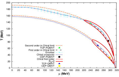
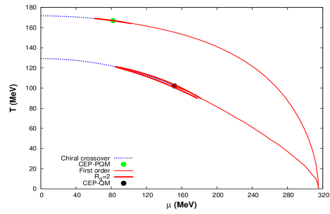
Figure 1: (a) For calculations with experimental pion mass, solid lines representing the first order chiral phase transition merge with the dotted lines (blue in color) for the chiral crossover at the CEP which is denoted by the filled circle. The thick solid lines around CEP are the contours of constant normalized quark number susceptibility $R_{q}$=2. For calculations with zero pion masss, dash lines represent the first order phase transition in the chiral limit of QMVT and PQMVT models while dash dot lines represent the second order transition and the filled triangle is the location of TCP where these two lines merge into each other. Lower part of the Fig. shows the QMVT model results while upper part shows the PQMVT results. (b) Lower part of the Fig. shows the QM model results while upper part shows the PQM results. The line types represent the same thing as in Fig.a for calculations with experimental pion mass.

The filled circle in the lower part of Fig.1 locates the CEP in QM model at $T_{CEP}$=102.09 MeV and $\mu_{CEP}$=151.7 MeV and again in the influence of Polyakov loop potential, the CEP in PQM model shifts considerably towards the temperature axis at $T_{CEP}$=166.88 MeV and $\mu_{CEP}$=81.02 MeV in the upper part of the Fig.1. If we compare the location of CEP in QM and PQM models as shown in Fig.1 to the location of CEP in QMVT and PQMVT models in Fig.1, we find a considerably significant shift of CEP to large chemical potential and small temperature values for QMVT and PQMVT models due to the robust influence of fermionic vacuum term inclusion in the effective potential. Another important thing worth noticing for the PQMVT model phase diagram in the upper part of Fig.1 is the highest value of temperature for the chiral crossover transition occurring on the temperature axis at $\mu=0$. The combined effect of Polyakov loop potential and fermionic vacuum term is responsible for this. If one compares the phase diagram in the lower part of Fig.1 for QM model with the phase diagram in the lower part of Fig.1 for QMVT model, one immediately notices that the the chiral crossover transition at $\mu=0$ occurs at a higher temperature value only due to the influence of fermionic vacuum fluctuation. These results are the extension of our recently reported workVivek:12 and facilitate the details of model comparison for the two quark flavour case. Further these results are also in qualitative agreement with the recent results of Schaefer et. al.Schaef:12 for the 2+1 flavour case.

For calculations with zero pion masss, dash lines represent the first order phase transition in the chiral limit of QMVT and PQMVT models in Fig.1 while dash dot lines represent the second order transition and the filled triangle is the location of TCP where these two lines merge into each other. In the upper part of the Fig.1, the filled triangle locates the presence of tricritical point (TCP) at $T_{t}$=137.09 MeV and $\mu_{t}$=240.14 MeV for PQMVT model calculation. In order to quantify the proximity of TCP to the CEP, we have plotted the constant normalized quark-number susceptibility ($R_{q}$=2) contour around CEP. It is seen on the phase diagram that the range and extension of this contour is quite large in both the directions;chemical potential as well as the temperature. The second cumulant of the net quark number fluctuations on this contour is double to that of the free quark gas value and such enhancements are the signatures of CEP for the heavy-ion collision experiments. The TCP location is quite well inside this contour on the phase diagram. It means that the shape of the critical region and nature of criticality around CEP, gets influenced by the presence of TCP in the corresponding chiral limit. In a recent NJL/PNJL model calculation by Costa et. al.Sousa , the CEP lies closer to the chemical potential axis but the TCP gets located on the periphery of $R_{q}$=2 contour around CEP. In the QMVT model calculation, the tricritical point (TCP) is found at $T_{t}$=69.06 MeV and $\mu_{t}$=263.0 MeV as denoted by filled triangle in the lower part of the Fig.1. Here also the TCP lies quite well inside the $R_{q}$=2 contour on the phase diagram.

III.1 Susceptibility Contours and Criticality

In order to locate the CEP in heavy-ion collision experiments, one requires the quantification of criticality around CEP. The crossover transition is marked by a peak in the quark number susceptibility which becomes sharper and higher as one approaches the CEP in the phase diagram from the crossover side and finally the peak diverges at CEP. Hence the quark number susceptibilities and scalar susceptibilities will be significantly enhanced in a region around the CEP in the $\mu$ and T plane in comparison to their respective values for the free quark gas. Thus the contour regions of properly normalized constant quark number susceptibilities and scalar susceptibilities, can be taken as the measure of criticality around CEP. The ratio of quark-number susceptibility $\chi_{q}$ normalized to the free susceptibility $\chi_{q}^{\text{free}}$ is written as:

$$R_{q}=\frac{\chi_{q}}{\chi_{q}^{\text{free}}}$$ (29)

The expression of quark number susceptibility is obtained as

$$\chi_{q}=-\frac{\partial^{2}\Omega_{\rm MF}}{\partial\mu^{2}}\,$$ (30)

$$\lim_{m_{q}\to 0}\chi_{q}(T,\mu)\!\!\! = \!\!\!\frac{\nu_{q}}{6}\left[T^{2}+\frac{3\mu^{2}}{\pi^{2}}\right]\equiv\chi_{q}^{\rm free}\,$$ (31)

$$\nu_{q}=2N_{c}N_{f}=12$$ (32)

The first and second partial derivatives of $\sigma$, $\Phi$ and $\Phi^{*}$ fields with respect to chemical potential contribute in the double derivatives of $\Omega(\sigma)$, $\cal U_{\text{log}}$ and $\Omega_{\mathrm{q\bar{q}}}^{\rm T}$ with respect to chemical potential as given in the appendix A of Ref.Vivek:12 .

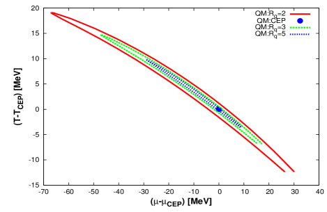
Figure 2: (a) The contours of three different values for the constant ratios $R_{q}=2,3$ and 5 of quark number susceptibility to the quark susceptibility for the free quark gas, are plotted in the PQM model calculations.(b) Similar contours plotted in the QM model calculations.

Contours with three different values for the ratios $R_{q}$, have been plotted in Fig.2 in the $\mu$ and T plane relative to the CEP. If we compare the contours in Fig.2 depicting the PQM model results to the contours in Fig.2 showing the pure QM model results, we conclude that the presence of Polyakov loop potential, compresses the critical region particularly in the T direction similar to findings of Schaefer et. al.Schaef:12 in their three flavour calculation. The compression of critical region in the T direction is much more pronounced in our two quark flavour calculation as can be seen in the spread of $R_{q}=2$ contour on the temperature axis only in a small range of $\pm 2.5$ MeV near $T_{CEP}$. The modification in the $\mu$-direction is quite moderate compared to the effect in the T direction. Since the chiral crossover transition becomes faster and sharper due to the presence Polyakov loop contribution in the effective potential, the critical region in the T direction gets significantly compressed.

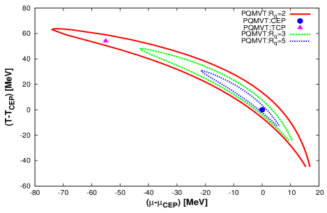
Figure 3: (a) The contours of three different values for the constant ratios $R_{q}=2,3$ and 5 of quark number susceptibility to the quark susceptibility for the free quark gas,are plotted in the PQMVT model calculations.(b) Similar contours as plotted in the QMVT model calculations.

The size of the critical region is significantly influenced by the incorporation of fermionic vacuum fluctuations in the effective potential as shown in Fig.3. In the phase diagram, the size of critical region is increased in a direction perpendicular to the crossover line due to the influence of the fermionic fluctuations. This effect is less pronounced in Fig.3 because of the compression of critical region width due to the presence of Polyakov loop potential contribution in PQMVT model while the QMVT model results of Fig.3 obtained in the absence of Polyakov loop, show a robust increase in the width of the critical region. However, the extent and size of critical region in the PQMVT model in Fig.3 is noticeably larger in both the directions $\mu$ as well as T compared to that of QMVT model results as shown in Fig.3. In the presence of fermionic vacuum term, CEP gets located at larger chemical potentials in QMVT/PQMVT models. Since the quark determinant gets modified mostly at moderate chemical potentials by the presence of Polyakov loop potential and further in its influence, the PQMVT model CEP shifts to a higher critical temperature [cf. also Fig.1] when compared to the CEP in QMVT model, we obtain an enhancement of the critical region in PQMVT model.Further the chiral crossover transition becomes much smoother because the phase transitions in general get washed out in the influence of fluctuations. This leads to a critical region which is broader in perpendicular direction to the extended first-order transition line. The influence of the Polyakov loop potential becomes insignificant for smaller temperatures and larger chemical potentials, hence the size of the critical region for $(\mu-\mu_{CEP})>0$ becomes comparable in both the models QMVT and PQMVT. In Fig.3, filled circles are the position of CEP and the filled triangles, show the location of TCP, we observe that the TCP gets located outside $R_{q}=3$ and quite well inside the $R_{q}=2$ contour.

If we compare our two quark flavour results with the 2+1 flavour calculations in renormalized PQM/QM models in Ref.Schaef:12 , we notice that in the absence of strange quarks, the effect of fermionic vacuum term, leads to an enhanced critical region in both the directions T as well as $\mu$ and the size of contours is larger in our two flavour calculation. We point out that the 2+1 flavour calculation in Ref.Schaef:12 was done with $m_{\sigma}=400$ MeV and $T_{0}=270$ MeV while in our two flavour calculation $m_{\sigma}=500$ MeV and $T_{0}=208$ MeV. In general higher value of $m_{\sigma}$ pushes the CEP to higher chemical potential. In our two quark flavour calculation, the CEP is at ($T_{CEP},\mu_{CEP}$)=(83.0,295.217) MeV and (32.24,299.35) MeV respectively in PQMVT and QMVT model calculations while the CEP in the corresponding the 2+1 flavour model calculation of Ref.Schaef:12 is at ($T_{CEP},\mu_{CEP}$)=(90.0,283.0) MeV and (32,286) MeV.

The zero-momentum projection of the scalar propagator, encodes all fluctuations of the order parameter and it corresponds to the scalar susceptibility $\chi_{\sigma}$. The relation of the scalar susceptibility to the order parameter is obtained asHatta ; Fujii ; Ohtani ; Schaefer:2006ds .

$$\chi_{\sigma}=-\frac{\partial^{2}\Omega_{\rm MF}}{\partial h^{2}}\$$ (33)

The most rapid change of the chiral order parameter, should be coincident with the maximum in the temperature or quark chemical potential variation of $\chi_{\sigma}$. The relation of scalar susceptibility to the sigma mass via $\chi_{\sigma}\sim m_{\sigma}^{-2}$ can be easily verified. The normalized scalar susceptibility is written asSchaefer:2006ds

$$R_{s}(T,\mu)=\frac{\chi_{\sigma}(T,\mu)}{\chi_{\sigma}(0,0)}$$ (34)

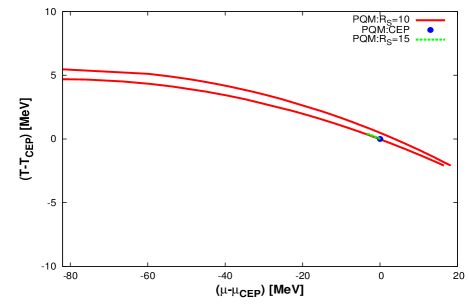
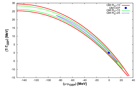
Figure 4: (a) The contours of different values for the constant ratios $R_{S}=10$ and 15 of T and $\mu$ dependent scalar susceptibility to the scalar susceptibility at T=0 and $\mu$=0 MeV, are plotted in the PQM model calculations.(b) Similar contours for the constant ratios $R_{S}=10,15$ and 25 are plotted in the QM model calculations.

In Fig. 4, the contours have been plotted for three values of fixed ratios $R_{s}$ around the CEP in the PQM and QM models. The $R_{s}=10$ contour in Fig. 4 is compressed in the T direction and its extension in $\mu$ direction is also reduced in comparison to the pure QM model contours in Fig. 4. This is due to the quite fast and rapid temperature or chemical potential variation of $\sigma$ meson mass $m_{\sigma}$ on account of faster and sharper change of order parameter for chiral crossover in the presence of Polyakov loop potential in the calculations. We do not find contour for $R_{s}=25$ in Fig. 4 because the minimum value of $\sigma$ meson mass does not fall below 100 MeV, though the value of $m_{\sigma}$ falls very rapidly and sharply from 500 MeV to 128 MeV giving rise to a very thin and small contour region even for $R_{s}=15$. In the QM model calculations, we get all the contour regions for $R_{s}=10,15$ and 25 with well defined size because the $m_{\sigma}$ variation is smoother and slower in comparison to the corresponding PQM model results and further the minimum in the $m_{\sigma}$ variation approaches almost zero value in QM model. The chiral crossover transition on the temperature axis at $\mu=0$ MeV in the QM and PQM models, is quite sharp and fast because it emerges from the background of first order chiral transition at $\mu=0$ MeV in the corresponding chiral limit of zero pion mass and we do not find the existence of TCP in QM/PQM models. As a consequence, we do not find the closure of $R_{s}=10$ contour on the temperature axis at $\mu=0$ MeV.

We obtain quite well defined and closed contour regions for $R_{s}=10,15$ and 25 in Fig. 5 which again become broader in the direction perpendicular to the crossover line due to the presence of fermionic vacuum fluctuations in QMVT and PQMVT model calculations. For scalar susceptibility also, the critical region gets elongated in the phase diagram and $\chi_{\sigma}$ is enhanced in the direction parallel to the first-order transition line. Here also the presence of Polyakov loop potential in the PQMVT model, leads to the compression in the width of critical region around CEP as shown in Fig.5. The fermionic vacuum fluctuations, make the chiral crossover transition very smooth while the Polyakov loop potential makes it sharper and faster and these opposite effects give a typical shape to the quark number susceptibility contours in Fig.3 in the PQMVT model. Similar effects can be seen in the scalar susceptibility contours in Fig.5. In the influence of fermionic vacuum fluctuations only, the $\chi_{\sigma}$ contours in Fig.5 in the pure QMVT model are broader and rounded.

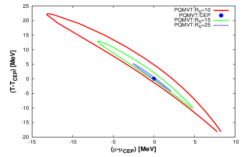
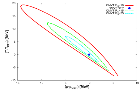
Figure 5: (a) The contours of three different values for the constant ratios $R_{S}=10,15$ and 25 of T and $\mu$ dependent scalar susceptibility to the scalar susceptibility at T=0 and $\mu$=0 MeV,are plotted in the PQMVT model calculations.(b)Similar contours for the constant ratios $R_{S}=10,15$ and 25 are plotted in the QMVT model calculations.

For the detail understanding and analysis of the criticality around the CEP, we will be studying the critical exponents of the susceptibilities at the critical point in the next section.

III.2 Critical Exponents

The crossover transition is marked by a peak in the quark number susceptibility which diverges as one approaches the CEP from the crossover side in the phase diagram. This divergence is governed by a power law within the critical region. The corresponding critical exponents depend on the route through which the singularity (CEP) is approached in the $\mu$ and T plane Griffiths1970 . This path dependence decides the shape of the critical region. In the mean-field approximation, the quark number susceptibility scales with an exponent $\gamma_{q}=1$ for a path asymptotically parallel to the first-order transition line and for any other path which is not parallel to the first-order line,the divergence scales with the exponent $\epsilon=2/3$. This larger critical exponent ($\gamma_{q}>\epsilon$) is one reason for the elongation of the critical region in a direction parallel to the first-order line as already pointed out inHatta ; Schaefer:2006ds .

In order to further investigate the nature of criticality in two flavour calculations, we have numerically evaluated the critical exponents of the quark number susceptibility $\chi_{q}$ in QM,PQM,QMVT and PQMVT models. In these investigations, the critical $\mu_{CEP}$ at fixed critical temperature $T_{CEP}$ is approached from the lower as well as higher $\mu$ sides in a path parallel to the $\mu$-axis in the ($T,\mu$)-plane. The calculation of the critical exponents, has been done with the following linear logarithmic fit formula:

$$\log\chi_{q}=-m\log|\mu-\mu_{CEP}|+c\ ,$$ (35)

The slope m gives the critical exponent $\epsilon$ and the Y axis intercept $c$ is independent of $\mu$.

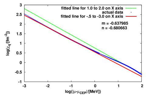
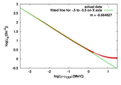
Figure 6: (a) Shows the plot of the logarithm of $\chi_{q}$ as a function of the logarithm of $\mu-\mu_{CEP}$ close to the CEP in QM model when the $\mu_{CEP}$ is approached from the lower $\mu$ side (b) shows the same plot as in Fig.a in QM model when the $\mu_{CEP}$ is approached from the higher $\mu$ side.

Fig. 6 shows the logarithm of $\chi_{q}$ as a function of the logarithm of $\mu-\mu_{CEP}$ close to the CEP in QM model. Scaling is observed over several orders of magnitude. In Fig. 6, the $\mu_{CEP}$ is approached from the lower $\mu$ side and we obtain a critical exponent $\epsilon=m=0.6379\pm 0.0002$ while the critical exponent $\epsilon=m=0.6648\pm 0.0001$ in the result of Fig. 6 when the $\mu_{CEP}$ is approached from the higher $\mu$ side. The scaling starts around around $\log|\mu-\mu_{CEP}|<-.5$ in both the cases. These exponents show good agreement with the mean-field prediction $\epsilon=2/3$. In Fig. 6, the data fitted in a range $1.0<\log|\mu-\mu_{CEP}|<2.0$ also shows a scaling kind of linear behaviour over one order of magnitude with a larger slope $n=.6807\pm.0002$ which changes to $m=.6379\pm.0002$ in the range $-.5<\log|\mu-\mu_{CEP}|<1.0$. When $log|\mu-\mu_{CEP}|\sim 2.0$, we are very close to $\mu=0$ on the temperature axis. The phase transition in the chiral limit at $\mu=0$ in QM model is first order and it becomes crossover for the real life pion mass. In the quark mass (or the pion mass) and T plane at $\mu=0$, the first order transition line should change to crossover line through another second order critical end point as one increases the pion mass from zero to the experimental value. This linear behaviour in a range $1.0<\log|\mu-\mu_{CEP}|<2.0$ with larger slope may be due to the influence of another hidden CEP in the mass and temperature plane at $\mu=0$ in the QM model. The critical exponent values obtained in PQM model calculation have been given in Table.1, we can see that the presence of Polyakov loop potential in QM model, does not influence the value of critical exponents.

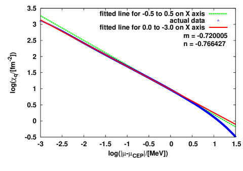
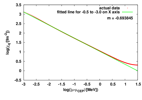
Figure 7: (a) Shows the plot of the logarithm of $\chi_{q}$ as a function of the logarithm of $\mu-\mu_{CEP}$ close to the CEP in QMVT model when the $\mu_{CEP}$ is approached from the lower $\mu$ side (b) shows the same plot as in Fig.a in QMVT model when the $\mu_{CEP}$ is approached from the higher $\mu$ side.

Fig. 7 shows the plot of the logarithm of $\chi_{q}$ with respect to the logarithm of $\mu-\mu_{CEP}$ in the presence of fermionic vacuum fluctuations in QMVT model. In Fig. 7 when the $\mu_{CEP}$ is approached from the lower $\mu$ side, we obtain a larger critical exponent $\epsilon=m=0.720\pm 0.00005$ in comparison to the corresponding result in the QM model. Due to the influence of fermionic vacuum fluctuation, we find the presence of TCP in the chiral limit of QMVT model and it lies quite well within the $R_{q}=2$ contour surrounding the CEP in the phase diagram in Fig. 1. This larger critical exponent may be the consequence of the modification of criticality around CEP due to the presence of TCP in its proximity. The scaling starts earlier when $\log|\mu-\mu_{CEP}|<0.0$ and we observe scaling over several orders of magnitude. This higher value of the critical exponent is close to the critical exponent calculated in Ref.Schaefer:2006ds where the effect of quantum fluctuations in the QM model were incorporated in the Proper-Time Renormalization Group (PTRG) approach. The critical exponents change in the range $-0.5<\log|\mu-\mu_{CEP}|<.5$ in Ref. Schaefer:2006ds , from .77 for the one scaling regime starting after $\log|\mu-\mu_{CEP}|>.5$ to .74 for another scaling regime starting before $\log|\mu-\mu_{CEP}|<-.5$. Though we do not find analogous crossing behavior of the universality classes, the data points in our calculation show a bending trend and when we fit the data in a small range $-0.5<\log|\mu-\mu_{CEP}|<.5$, we find a higher slope $\epsilon=m=0.7664\pm 0.0002$ as shown in the Fig. 7. In our calculation, the critical region of CEP is having a noticeable overlap with the critical region of TCP and this may be the reason of the bending trend in the data. If we approach the CEP from the higher $\mu$ side, we find smaller critical exponent $\epsilon=m=0.6938\pm 0.0002$ in the result of Fig. 7. In this case, the scaling starts around $\log|\mu-\mu_{CEP}|<-.5$ . It is pointed out that these exponents calculated in the presence of fermionic vacuum fluctuations in the QM model are different from the mean-field prediction $\epsilon=2/3$. Similar results are found in Fig. 8 which shows the plot of the logarithm of $\chi_{q}$ with respect to the logarithm of $\mu-\mu_{CEP}$ in the presence of fermionic vacuum fluctuations in PQMVT model. The presence of Polyakov loop compresses the width of critical region in PQMVT model but its effect on critical exponents is negligibly small as can be seen in Fig. 8 and Fig. 8. We point out that the recent calculation in 2+1 flavour model in Ref.Schaef:12 does not report any modification of the mean field critical exponents under the infulence of fermionic vacuum term. The chiral crossover transition occurring at $\mu=0$ on the temperature axis, will be faster and sharper due to the presence of s quarks in their 2+1 quark flavour calculation if we compare the present two quark flavour calculation with that of them.

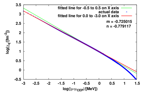
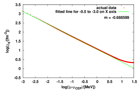
Figure 8: (a) shows the plot of the logarithm of $\chi_{q}$ as a function of the logarithm of $\mu-\mu_{CEP}$ close to the CEP in PQMVT model when the $\mu_{CEP}$ is approached from the lower $\mu$ side (b) shows the same plot as in Fig.a in PQMVT model when the $\mu_{CEP}$ is approached from the higher $\mu$ side.

The critical exponents calculated in all the models are summarized and tabulated in Table 1.

Model	$\mu-\mu_{CEP}<0$	$\mu-\mu_{CEP}>0$
QM	$0.6379\pm 0.0002$	$0.6648\pm 0.0001$
PQM	$0.6309\pm 0.0001$	$0.6668\pm 0.0001$
QMVT	$0.720\pm 0.00005$	$0.6938\pm 0.0002$
PQMVT	$0.725\pm 0.0002$	$0.6886\pm 0.0004$

Table 1: Critical exponents of the quark-number susceptibility in the QM,PQM,QMVT and PQMVT models for two different paths parallel to the chemical potential axis approaching the $\mu_{CEP}$ from the lower $\mu<\mu_{CEP}$ and higher $\mu>\mu_{CEP}$side.

III.3 In medium meson masses

The critical fluctuations are also encoded in the variation of meson masses $m_{\pi}(T,\mu)$ and $m_{\sigma}(T,\mu)$ as one passes through the chiral symmetry restoring phase transition. We will investigate and compare the ’in-medium’ meson mass variations in QM, QMVT and PQM, PQMVT models in order to see the influence of fermionic vacuum fluctuations. The sigma and pion masses are calculated by determining the curvature of grand potential at the global minimum.

$$m_{\pi,i}^{2}(T,\mu)=\frac{\partial^{2}\Omega(T,\mu)}{\partial\pi_{i}\partial\pi_{i}}\bigg{|}_{min}$$ (36)

$$m_{\sigma}^{2}(T,\mu)=\frac{\partial^{2}\Omega(T,\mu)}{\partial\sigma\partial\sigma}\bigg{|}_{min}$$ (37)

The left panel of Fig. 9 shows the temperature variations of meson masses for $\mu=0$, $\mu=\mu_{CEP}$ and $\mu>\mu_{CEP}$ in QM model while the right panel shows the corresponding variations in QMVT model. In the chiral symmetry broken mesonic phase, the sigma mass always decreases with temperature. Sigma mass increases again at high temperatures signaling chiral symmetry restoration and it becomes degenerate with the increasing pion mass which does not vary much below the transition temperature. The degenerate meson masses increase linearly with $T$ after the chiral symmetry restoration transitionSchaefer:2006ds has taken place.

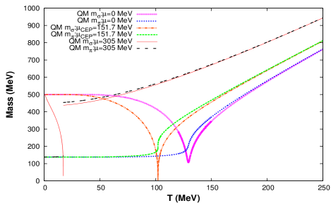
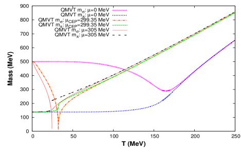
Figure 9: (a) Mass variations in the QM model are shown in this Fig. Two dotted lines in the rightmost part of the Fig. represent the temperature variations of $m_{\sigma}$ and $m_{\pi}$ at $\mu=0$, the dash dotted line in the middle part represents $m_{\sigma}$ while the line with small dash represents $m_{\pi}$ temperature variations at $\mu_{CEP}=151.7$ and the solid line in the leftmost part of the Fig. represents $m_{\sigma}$ while the line with dash represents $m_{\pi}$ temperature variations at $\mu=305$ MeV. (b) Temperature variations of $m_{\sigma}$ and $m_{\pi}$ in the influence of fermionic vacuum fluctuations, have been shown for the QMVT model calculations. Lines represent the same mass variations as in the left panel of the Fig. In QMVT model $\mu_{CEP}=299.35$ MeV.

The temperature variations of $m_{\sigma}$ and $m_{\pi}$ masses at $\mu=0$ in Fig. 9 are significantly modified due to the presence of fermionic vacuum fluctuations in QMVT model. If we compare these variations with the corresponding QM model temperature variations of masses in Fig. 9, we find that the mass degeneration in $m_{\sigma}$ and $m_{\pi}$ at $\mu=0$ in Fig. 9 becomes very smooth and it takes place at a higher temperature. Since the chiral crossover transition on the temperature axis at $\mu=0$ is quite sharp and fast in QM model, the mass degeneration trend in $m_{\sigma}$ and $m_{\pi}$ is also quite sharp and fast in Fig. 9. Fermionic vacuum fluctuations make the chiral crossover at $\mu=0$ very smooth in QMVT model and this gets reflected also in the setting up of a very smooth mass degeneration trend at $\mu=0$ in Fig. 9. Long-wavelength fluctuations of the order parameter, characterize the second-order phase transitions. Since the chiral phase transition turns second order at the CEP, the sigma meson mass must vanish at the CEP because the effective potential completely flattens in the radial direction. Thus the sigma meson mass drops below the pion mass near the CEP. We know that the CEP in QMVT model gets shifted to a significantly higher chemical potential under the influence of fermionic vacuum fluctuation, hence the sigma mass becomes almost zero at $\mu_{CEP}=299.35$ MeV in QMVT model as shown in Fig. 9. The sigma mass goes to zero only at $\mu_{CEP}=151.7$ MeV in Fig. 9 in QM model. The discontinuities in mass evolutions respectively in Fig. 9 and Fig. 9 , signal a first-order phase transition at small temperatures when $\mu>\mu_{CEP}=305$ MeV in both the models QM as well as QMVT.

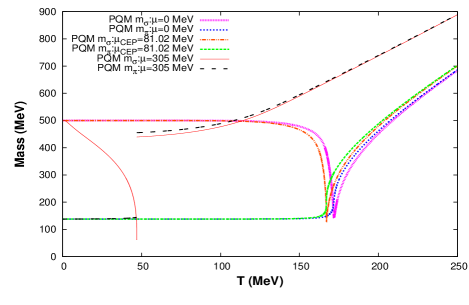
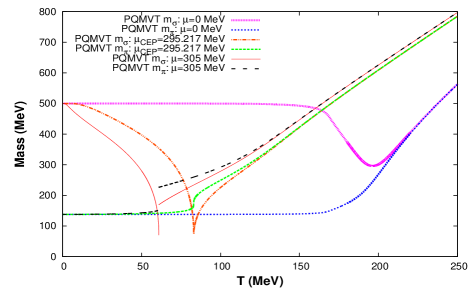
Figure 10: (a) Mass variations in the PQM model are shown in this Fig. Two dotted lines in the rightmost part of the Fig. represent the temperature variations of $m_{\sigma}$ and $m_{\pi}$ at $\mu=0$, the dash dotted line in the middle part represents $m_{\sigma}$ while the line with small dash represents $m_{\pi}$ temperature variations at $\mu_{CEP}=81.02$ MeV and the solid line in the leftmost part of the Fig. represents $m_{\sigma}$ while the line with dash represents $m_{\pi}$ temperature variations at $\mu=305$ MeV. (b) Temperature variations of $m_{\sigma}$ and $m_{\pi}$ in the influence of fermionic vacuum fluctuations, have been shown for the PQMVT model calculations. Lines represent the same mass variations as in the left panel of the Fig. In PQMVT model $\mu_{CEP}=295.217$ MeV.

Finally we will be investigating how the fermionic vacuum term influences the emergence of masss degeneration trend in $m_{\sigma}$ and $m_{\pi}$ as the chiral symmetry restoring transition takes place in the presence of Polyakov loop potential. Fig. 10 presents temperature variations of meson masses at $\mu=0$, $\mu=\mu_{CEP}$ and $\mu>\mu_{CEP}$ in the in PQM model calculations while Fig. 10 shows the corresponding mass variations in PQMVT model. Since the chiral crossover transition on the temperature axis at $\mu=0$ becomes very sharp and rapid in the PQM model due to the influence of Polyakov loop potential, the mass degeneration trend in $m_{\sigma}$ and $m_{\pi}$ at $\mu=0$ also becomes very sharp and fast in Fig. 10. Here in the PQMVT model calculations also as in the case of QMVT model, the mass degeneration in $m_{\sigma}$ and $m_{\pi}$ at $\mu=0$ becomes very smooth in the influence of fermionic vacuum fluctuations as shown in Fig. 10. Further this mass degeneration takes place at a temperature which is highest of the corresponding mass degeneration temperatures in other models. This happens because, the chiral crossover transition at $\mu=0$ occurs at a temperature which is highest in the PQMVT model calculations, due to the combined effect of Polyakov loop potential and fermionic vacuum term. We point out that the sigma meson mass neither vanishes nor becomes very close to zero at CEP as shown in Fig. 10 and Fig. 10 respectively for PQM and PQMVT model temperature variations. In PQM model, $m_{\sigma}$ in its temperature variation reaches the minimum value of 128 MeV as shown by the dash dotted line in Fig. 10 while in PQMVT model the minimum value reached in the temperature variation of $m_{\sigma}$ is 76.0 MeV as evident from the dash dotted line in Fig. 10. It means that the effective potential of PQM and PQMVT model does not completely flattens in the radial direction at the CEP. The Polyakov loop expectation value is a scalar field which mixes up with the chiral order parameter and this effect hampers the flattening of the PQM model effective potential in the radial direction (i.e. the direction of $\sigma$ field) at the CEP. In PQMVT model, this effect seems to be considerably remedied by the presence of the fermionic vacuum term and the minimum value of $m_{\sigma}$ becomes 76.0 MeV in its temperature variation. Here also, the discontinuities in mass evolutions respectively in Fig. 10 and Fig. 10 ,signal a first-order phase transition at small temperatures when $\mu>\mu_{CEP}=305$ MeV in both the models PQM as well as PQMVT.

IV Summary and Conclusion

In the beginning of the present work, we computed the phase diagrams and pin-pointed the CEP positions in the $\mu$ and T plane of all the four two quark flavor models QMVT,PQMVT,QM and PQM for the real life explicit chiral symmetry breaking with the experimental value of pion mass. We obtained the phase diagrams with zero pion mass also for the chiral limit in the QMVT and PQMVT models and located the respective positions of TCP. Since the presence or absence of TCP in the phase diagram and its distance from CEP in a model calculation, influences the nature of critical fluctuations around CEP, we quantified the proximity of TCP to the CEP in the phase diagrams obtained for QMVT and PQMVT model calculations.

The QMVT model CEP is positioned at $\mu_{CEP}$=299.35 MeV and $T_{CEP}$=32.24 MeV and it shifts to higher temperature $T_{CEP}$=83.0 MeV and lower chemical potential $\mu_{CEP}$=295.217 MeV in PQMVT model due to the effect of Polyakov loop. In QM model, the CEP is located at $T_{CEP}$=102.09 MeV and $\mu_{CEP}$=151.7 MeV and again in the influence of Polyakov loop potential, it shows considerable shift towards the temperature axis in PQM model and gets located at $T_{CEP}$=166.88 MeV and $\mu_{CEP}$=81.02 MeV. If we compare the location of CEP in QM and PQM models to the location of CEP in QMVT and PQMVT models, we find a considerably significant shift of CEP to large chemical potential and small temperature values for QMVT and PQMVT models due to the robust influence of fermionic vacuum term presence in the effective potential. In chiral limit of PQMVT model, the tricritical point(TCP) exists at $T_{t}$=137.09 MeV and $\mu_{t}$=240.14 MeV and the TCP in QMVT model is found at $T_{t}$=69.06 MeV and $\mu_{t}$=263.0 MeV. The proximity of TCP to the CEP has been quantified by plotting the constant normalized quark-number susceptibility ($R_{q}$=2) contours around CEP in the phase diagrams of PQMVT and QMVT models. The second cumulant of the net quark number fluctuations on these contours is double to that of the free quark gas value and such enhancements are the signatures of CEP for the heavy-ion collision experiments. The TCP location is quite well inside the $R_{q}$=2 contour on the phase diagram of both the models QMVT as well as PQMVT.

The CEP in phase diagrams is pin-pointed by tracking down the divergence in the quark number susceptibilities and scalar susceptibilities which show significant enhancement in a region around the CEP in the $\mu$ and T plane in comparison to their respective values for the free quark gas. In order to determine the shape of the critical region around CEP, we have plotted different contour regions having different constant values of properly normalized quark number susceptibility ratio ($R_{q}$) and scalar susceptibility ratio ($R_{S}$). The different shapes of these contours as calculated in various models, throw light on the nature of criticality around CEP in those models. We have plotted the contours with three different values of quark number susceptibility ratio $R_{q}=2,3$ and 5, in the $\mu$ and T plane relative to the CEP. If we compare the contours obtained in the PQM model to the contours in pure QM model, we conclude that the presence of Polyakov loop potential, compresses the critical region particularly in the T direction. Since the chiral crossover transition becomes faster and sharper due to the presence of Polyakov loop potential, the critical region in the T direction gets significantly compressed. The analysis of the shape of $R_{q}=2,3$ and 5 contours in the QMVT and PQMVT models, tells us that the size of critical region is increased in a direction perpendicular to the crossover line due to the influence of the fermionic vacuum fluctuations. This effect is less pronounced in PQMVT model because of the compression of critical region width due to the presence of Polyakov loop potential while the QMVT model contours show a robust increase in the width of the critical region in perpendicular direction to the crossover transition line . However, the extent and size of critical region in the PQMVT model is noticeably larger in both the directions $\mu$ as well as T compared to that of QMVT model results. In the presence of fermionic vacuum term, CEP gets located at larger chemical potentials in QMVT/PQMVT models. Since the quark determinant gets modified mostly at moderate chemical potentials by the presence of Polyakov loop potential and further in its influence, the PQMVT model CEP shifts to a higher critical temperature when compared to the CEP in QMVT model, we obtain an enhancement of the critical region in PQMVT model.

We have plotted three contours around the CEP in PQM and QM models also for the normalized scalar susceptibility ratios $R_{s}=10,15$ and 25. The shape of $R_{s}=10$ contour in PQM model is compressed in comparison to the pure QM model contours. The $R_{s}=25$ contour is not obtained in PQM model calculation because the minimum value of $\sigma$ meson mass does not fall below 100 MeV. Since the value of $m_{\sigma}$ falls very rapidly and sharply from 500 MeV to 128 MeV, we obtain a very thin and small contour region even for $R_{s}=15$. We get all the contours regions for $R_{s}=10,15$ and 25 with well defined size in the QM model calculations because the $m_{\sigma}$ variation is smoother and slower in comparison to the corresponding PQM model results and further the minimum in the $m_{\sigma}$ variation approaches almost zero value in QM model. Further we do not find the closure of $R_{s}=10$ contour on the temperature axis at $\mu=0$ MeV in both the models QM as well as PQM. We obtain quite well defined and closed contour regions for $R_{s}=10,15$ and 25 in QMVT and PQMVT model calculations which again become broader in the direction perpendicular to the crossover line due to the presence of fermionic vacuum fluctuations. For scalar susceptibility also, the critical region gets elongated in the phase diagram and $\chi_{\sigma}$ is enhanced in the direction parallel to the first-order transition line. Here also the presence of Polyakov loop potential in the PQMVT model, leads to the compression in the width of critical region around CEP.The fermionic vacuum fluctuations, make the chiral crossover transition very smooth while the Polyakov loop potential makes it sharper and faster and these opposite effects give a typical shape to the quark number susceptibility contours in the PQMVT model. Similar effects can be seen in the scalar susceptibility contours also. In the influence of fermionic vacuum fluctuations only, the $\chi_{\sigma}$ contours in the pure QMVT model are broader and rounded.

In order to further investigate the nature of criticality in two flavour calculations, we have numerically evaluated the critical exponents of the quark number susceptibility $\chi_{q}$ in QM,PQM,QMVT and PQMVT models. In these investigations, the critical $\mu_{CEP}$ at fixed critical temperature $T_{CEP}$ is approached from the lower as well as higher $\mu$ sides in a path parallel to the $\mu$-axis in the ($T,\mu$)-plane. The calculation of the critical exponents has been done using the linear logarithmic fit. If the $\mu_{CEP}$ is approached in QM model from the lower $\mu$ side, we obtain a critical exponent equal to $\epsilon=0.6379\pm 0.0002$ while the critical exponent is $\epsilon=0.6648\pm 0.0001$ when the $\mu_{CEP}$ is approached from the higher $\mu$ side. The scaling starts around around $\log|\mu-\mu_{CEP}|<-.5$ in both the cases. These exponents show good agreement with the mean-field prediction $\epsilon=2/3$. The influence of Polyakov loop potential on the calculated values of critical exponents in PQM model, is negligible and we obtain similar critical exponents as evaluated in QM model.

If the $\mu_{CEP}$ in QMVT model calculation is approached from the lower $\mu$ side, we obtain a critical exponent $\epsilon=m=0.720\pm 0.00005$ which is larger in comparison of the corresponding critical exponent $\epsilon=0.6379\pm 0.0002$ evaluated in the QM model. Due to the influence of fermionic vacuum fluctuation, we find the presence of TCP in the chiral limit of QMVT model and it lies quite well within the $R_{q}=2$ contour surrounding the CEP in the phase diagram. This larger critical exponent may be the consequence of the modification of criticality around CEP due to the presence of TCP in its proximity. The scaling starts earlier when $\log|\mu-\mu_{CEP}|<0.0$ and we observe scaling over several orders of magnitude. We obtain smaller critical exponent $\epsilon=0.6938\pm 0.0001$ when the $\mu_{CEP}$ is approached from the higher $\mu$ side in PQMVT model. It is pointed out that these exponents calculated in the presence of fermionic vacuum fluctuations in the QM model are different from the mean-field prediction $\epsilon=2/3$. The presence of Polyakov loop compresses the width of critical region in PQMVT model but its effect on critical exponents is negligible. The critical exponents obtained in PQM model calculations are also similar to the critical exponents of QM model.

Since the critical fluctuations are encoded in the variation of meson masses $m_{\pi}(T,\mu)$ and $m_{\sigma}(T,\mu)$ as one passes through the chiral symmetry restoring phase transition, we have also investigated and compared the ’in-medium’ meson mass temperature variations for $\mu=0$, $\mu=\mu_{CEP}$ and $\mu>\mu_{CEP}$ in QM, QMVT and PQM, PQMVT model calculations. If we compare the temperature variations of masses at $\mu=0$ in QM and QMVT model calculations, we find that the mass degeneration in $m_{\sigma}$ and $m_{\pi}$ at $\mu=0$ becomes very smooth in QMVT model and it takes place at a higher temperature. Since the sharper and faster chiral crossover transition occurring on the temperature axis at $\mu=0$ in QM model, becomes very smooth in QMVT model under the influence of fermionic vacuum fluctuations, the sharper mass degeneration trend in $m_{\sigma}$ and $m_{\pi}$ in QM model also becomes a very smooth mass degeneration trend in QMVT model. The sigma meson mass must vanish at the CEP since the chiral phase transition turns second order at this point and the effective potential completely flattens in the radial direction. In our QM and QMVT model calculations, we have shown that the sigma meson mass becomes almost zero at $\mu=\mu_{CEP}$. in both the models. It has also been shown that the discontinuities in mass evolutions, signal a first-order phase transition at small temperatures when $\mu>\mu_{CEP}=305$ MeV in both the models QM as well as QMVT.

Finally our investigation gets concluded by the study of the influence of Polyakov loop potential on the emergence of masss degeneration trend in $m_{\sigma}$ and $m_{\pi}$ as the chiral symmetry restoration takes place in the presence of fermionic vacuum fluctuation. Since the chiral crossover transition on the temperature axis at $\mu=0$ becomes very sharp and rapid in the PQM model due to the influence of Polyakov loop potential, the mass degeneration trend in $m_{\sigma}$ and $m_{\pi}$ at$\mu=0$ also becomes very sharp and fast in PQM model. Here in the PQMVT model calculations also as in the case of QMVT model, the mass degeneration in $m_{\sigma}$ and $m_{\pi}$ at $\mu=0$ becomes very smooth in the influence of fermionic vacuum fluctuations. Further this mass degeneration happens at a temperature which is highest of the corresponding mass degeneration temperatures in other models. In the PQMVT model calculations, we obtain highest temperature for chiral crossover transition on the temperature axis at $\mu=0$. The combined effect of Polyakov loop potential and fermionic vacuum term is responsible for this. We point out that the sigma meson mass neither vanishes nor becomes very close to zero at $\mu=\mu_{CEP}$ in PQM and PQMVT model temperature variations. In PQM model, $m_{\sigma}$ in its temperature variation reaches the minimum value of 128.0 MeV while the minimum value reached in the temperature variation of $m_{\sigma}$ in PQMVT model is 76.0 MeV. It means that the effective potential of PQM and PQMVT model does not completely flattens in the radial direction at the CEP. The Polyakov loop expectation value is a scalar field which mixes up with the chiral order parameter and this effect hampers the flattening of the PQM model effective potential in the radial direction (i.e. the direction of $\sigma field)$ at the CEP. In the PQMVT model, this effect seems to be considerably remedied by the presence the fermionic vacuum term and we get minimum in $m_{\sigma}$ temperature variation at 76.0 MeV. We have also shown the discontinuities in mass evolutions which signal a first-order phase transition at small temperatures when $\mu>\mu_{CEP}=305$ MeV in both the models PQM as well as PQMVT.

References

D. H. Rischke, Prog. Part. Nucl. Phys.52, 197 (2004).

H.Meyer-Ortmanns Rev. Mod. Phys. 68, 473 (1996).

B.Muller, Rep. Prog. Phys. 58, 611 (1995).

L.D.McLerran, B.Svetitsky, Phys. Rev. D24, 450 (1981); B.Svetitsky, Phys. Rep. 132, 1 (1986).

A. M. Polyakov, Phys. Lett. B 72, 477 (1978).

R. D. Pisarski, Phys. Rev. D 62 111501(R) (2000).

B. Layek, A. P. Mishra, A. M. Srivastava and V. K. Tiwari, Phys. Rev. D 73 103514 (2006).

A.Ali Khan et al. Phys. Rev. D 64, 074510 (2001).

F. Karsch, Lect. Notes Phys. 583, 209 (2002).

P. de Forcrand and O. Philipsen, Nucl. Phys. B642, 290 (2002).

Z. Fodor and S. D. Katz Phys. Lett. B 534, 87 (2002); Z. Fodor, S. D. Katz, and K. K. Szabo, Phys. Lett. B 568, 73 (2003).

C. R. Allton, S. Ejiri, S. J. Hands, O. Kaczmarek, F. Karsch, E Laermann and C. Schmidt, Phys. Rev. D 68, 014507 (2003); C. R. Allton, M. Doring, S. Ejiri, S. J. Hands, O. Kaczmarek, F. Karsch, E Laermann and K. Redlich, Phys. Rev. D 71, 054508 (2005).

Y. Aoki, Z. Fodor, S. D. Katz and K. K. Szabo, Phys. Lett. B 643, 46 (2006); Y. Aoki et al., J. High Energy Phys.06 (2009) 088

F. Karsch, J. Phys. G 31, S633 (2005).

F. Karsch, e-Print: arXiv:0701.210 [hep-ph].

M. Cheng et al., Phys. Rev. D 74, 054507 (2006).

M. Cheng et al., Phys. Rev. D 77, 014511 (2008).

S. Digal, E. Laermann and H. Satz, Eur. Phys. J. C 18, 583 (2001).

A. Bazavov et al., arXiv:1111.1710; S. Borsanyi et. al., J. High Energy Phys. 09 (2010) 073.

R. D. Pisarski and F. Wilczek Phys. Rev. D 29, 338 (1984).

M. Asakawa and K. Yazaki, Nucl. Phys. A504, 668 (1989).

A. Barducci, R. Casalbuoni, S. De Curtis, R. Gatto and G. Pettini, Phys. Lett. B 231, 463 (1989); A. Barducci, R. Casalbuoni, S. De Curtis, R. Gatto and G. Pettini, Phys. Rev. D 41, 1610 (1990).

J. Berges and K. Rajagopal, Nucl. Phys. B538, 215 (1999).

Y. Hatta and T. Ikeda, Phys. Rev. D 67, 014028 (2003).

H. Fujii, Phys. Rev. D 67, 094018 (2003).

K. Fukushima,arXiv:1008.4322

D. T. Son and M. A. Stephanov, Phys. Rev. D 70, 056001 (2004); Y. Aoki, G. Androdi, Z. Fodor, S. D. Katz and K. K. Szabo, Nature (London) 443,675 (2006); S. Gupta, X. Luo, B. Mohanty, H. G. Ritter and N. Xu Science 332,1525 (2011).

O. Philipsen, arXiv:1111.5370.

M. A. Stephanov, K. Rajagopal and E. V. Shuryak, Phys. Rev. D 60, 114028 (1999); Phys. Rev. Lett.81, 4816 (1998).

S. Jeon and V. Koch, Phys. Rev. Lett.85, 2076 (2000); in Quark Gluon Plasma edited by R. C. Hwa (World Scientific, Singapore,2004),p. 430

S. Ejiri, F. Karsch and K. Redlich, Phys. Lett.B633, 275 (2006).

J. Adams et al. (STAR Collaboration) Nucl. Phys. A757, 102 (2005), M. Aggarwal et al. (STAR Collaboration), Phys. Rev. Lett.105, 022302 (2010).

B. Mohanty, Nucl. Phys. A830, 899c (2009).

V. Koch, arXiv:0810.2520.

X. Luo, B. Mohanty, H. G. Ritter and N. Xu, arXiv:1105.5049.

J. T. Lenaghan, D. H. Rischke and J. Schaffner-Bielich, Phys. Rev D 62, 085008 (2000). J. T. Lenaghan, D. H. Rischke, J. Phys. G 26, 431 (2000).

S. Chiku and T. Hatsuda, Phys. Rev. D 58, 076001 (1998).

S. Chiku Prog. Theor. Phys. 104, 1129 (2000).

T. Herpay, A. Patkós, Zs. Szép and P. Szépfalusy, Phys. Rev. D 71, 125017 (2005).

T. Herpay and Zs. Szép, Phys. Rev. D 74, 025008 (2006).

P. Kovács and Zs. Szép, Phys. Rev. D 75, 025015 (2007).

G. Fejos, A. Patkos, Phys. Rev. D 82, 045011 (2010).

O. Scavenius, A. Mocsy, I. N. Mishustin, D. H. Rischke, Phys. Rev. C 64, 045202 (2001).

B. J. Schaefer and M. Wagner, Phys. Rev. D 79, 014018 (2009).

J. O. Andersen, R. Khan and L. T. Kyllingstad, AIP Conf. Proc. 1343 :504-506 (2011) e-Print: arXiv:1102.2779 [hep-ph]

A. Jakovac, A. Patkos, Z. Szep, and P. Szepfalusy, Phys. Lett. B 582, 179 (2004).

A. Mocsy, I. N. Mishustin, and P. J. Ellis, Phys. Rev. C 70, 015204 (2004).

B.-J. Schaefer and J. Wambach, Nucl. Phys. A 757, 479 (2005).

B.-J. Schaefer and J. Wambach, Phys. Rev. D 75, 085015 (2007).

P. Kovacs and Zs. Szep, Phys. Rev. D 75, 025015 (2007).

E. S. Bowman and J. I. Kapusta, Phys. Rev. C 79, 015202 (2009); J. I. Kapusta, and E. S. Bowman, Nucl. Phys.  A 830, 721C (2009).

A. Jakovac and Zs. Szep, Phys. Rev. D 82, 125038, (2010).

L. Ferroni, V. Koch, and M. B. Pinto, Phys. Rev. C 82, 055205 (2010).

P. Costa, M. C. Ruivo, C. A. de Sousa Phys. Rev. D 77, 096001 (2008).

J.-L Kneur, M. B. Pinto and R.O. Ramos, Phys. Rev. C 81, 065205 (2010).

T. Kahara and K. Tuominen, Phys. Rev. D 78, 034015 (2008); ibid D 80, 114022 (2009). ibid D 82, 114026 (2010).

D. Nickel, Phys.Rev. D 80, 074025 (2009).

S. Rößner, C. Ratti, and W. Weise, Phys. Rev. D 75, 034007 (2007).

C. Ratti, M. A. Thaler and W. Weise, Phys. Rev. D 73, 014019 (2006).

S. Rößner, T. Hell, C. Ratti, and W. Weise, Nucl. Phys. A 814, 118 (2008).

S. K. Ghosh, T. K. Mukherjee, M. G. Mustafa and R. Ray, Phys. Rev. D 73, 114007 (2006).

C. Sasaki, B. Friman and K. Redlich, Phys. Rev D 75, 074013 (2007).

T. Hell, S. Rößner, M. Cristoforetti and W. Weise, Phys. Rev D 79, 014022 (2009).

H. Abuki, R. Anglani, R. Gatto, G. Nardulli and M. Ruggieri, Phys. Rev D 78, 034034 (2008).

M. Ciminale, R. Gatto, N. D. Ippolito, G. Nardulli and M. Ruggieri, Phys. Rev D 77, 054023 (2008).

W.-J. Fu, Z. Zhang and Y.-X. Liu, Phys. Rev D 77, 014006 (2008).

K. Fukushima, Phys. Rev D 77, 114028 (2008).

K. Fukushima, Phys. Rev D 78, 114019 (2008).

K. Fukushima, Phys. Rev D 79, 074015 (2009).

H. Hansen, W. M. Alberico, A. Beraudo, A Molinari, M. Nardi and C. Ratti Phys. Rev. D 75, 065004 (2007).

P. Costa, M. C. Ruivo, C. A. de Sousa, H. Hansen and W. M. Alberico Phys. Rev. D 79, 116003 (2009).

K. Kashiwa, H. Kouno, and M. Matsuzaki, and M. Yahiro Phys. Lett. B 662, 26 (2008).

A. E. Radzhabov, D. Blaschke, M. Buballa, and M. K. Volkov, e-Print: arXiv:1012.0664 [hep-ph].

K. Fukushima, Phys. Lett. B 591, 277 (2004).

B. J. Schaefer, J. M. Pawlowski and J. Wambach, Phys. Rev. D 76, 074023 (2007).

B. J. Schaefer and M. Wagner, arXiv:0812.2855 [hep-ph].

B. J. Schaefer, M. Wagner and J. Wambach, e-Print: arXiv:0909.0289 [hep-ph]

B. J. Schaefer, M. Wagner and J. Wambach, Phys. Rev. D 81, 074013 (2010). e-Print: arXiv:0910.5628 [hep-ph]

H. Mao, J. Jin and M. Huang, J. Phys. G 37, 035001 (2010).

U. S. Gupta and V. K.Tiwari, Phys. Rev. D 81, 054019 (2010).

G. Marko and Zs. Szep, Phys. Rev.D 82, 065021 (2010).

V. Skokov, B. Friman, E. Nakano, K. Redlich, and B.-J. Schaefer, Phys. Rev. D 82, 034029 (2010).

T. K. Herbst, J. M. Pawlowski, and B.-J. Schaefer. Phys. Lett. B 696, 58 (2011).

A. Barducci, R. Casalbuoni, G. Pettini and R. Gatto, Phys. Rev. D 49, 426 (1994).

M. A. Halasz, A. D. Jackson, R. E. Shrock, M. A. Stephanov and J. J. M. Verbaarschot, Phys. Rev. D 58, 096007 (1998).

M. Harada, and A. Shibata, Phys. Rev. D 59, 014010 (1998).

N. Brouzakis and N. Tetradis Nucl. Phys.A 742, 144 (2004).

C. Nonaka and M. Asakawa, Phys. Rev. C 71, 044904 (2005).

H. Fujii and M. Ohtani, Phys. Rev. D 70, 014016 (2004).

P. Costa, C.A. de Sousa, M.C. Ruivo and H. Hansen, Europhys. Lett. 86, 31001 (2009).

A. J. Mizher, M. N. Chernodub and E. S. Fraga, Phys. Rev. D 82, 105016 (2010).

L. F. Palhares and E. S. Fraga, Phys. Rev.  D 78, 025013 (2008) [arXiv:0803.0262 [hep-ph]].

E. S. Fraga, L. F. Palhares and M. B. Pinto, Phys. Rev.  D 79, 065026 (2009) [arXiv:0902.1498 [hep-ph]].

L. F. Palhares and E. S. Fraga, Phys. Rev.  D 82, 125018 (2010) [arXiv:1006.2357 [hep-ph]].

U. S. Gupta and V. K.Tiwari, Phys. Rev. D 85, 014010 (2012).

B.-J. Schaefer and M. Wagner, Phys. Rev. D 85, 034027 (2012).

M. Quiros, arXiv:hep-ph/9901312.

R. B. Griffiths and J. Wheeler, Phys. Rev. A, 1047 (1970).