The Swift X–ray Telescope Cluster Survey: data reduction and cluster catalog for the GRB fields

Abstract

Aims. We present a new sample of X–ray selected galaxy groups and clusters serendipitously observed with the X–ray Telescope (XRT) on board of the Swift satellite. Using the XRT archive as of April 2010, we searched for extended sources among 336 GRB fields with galactic latitude $|b|>$20^∘. Our selection algorithm provides us with a flux-limited sample of 72 X–ray groups and clusters with a well defined selection function and an expected negligible contamination. The sky coverage of the survey goes from the total 40 deg² to 1 deg² at a flux limit of $10^{-14}$ erg s^-1 cm^-2 ($0.5-2$ keV). This paper provides a description of the XRT data processing, the statistical calibration of the survey, and the catalog of detected cluster candidates.

Methods. All the X–ray sources are detected in the Swift-XRT soft ($0.5-2$ keV) images with the algorithm wavdetect. A size parameter defined as the half power radius (HPR) measured inside a box of 45$\times$45 arcsec, is assigned to each source. We select extended sources by applying a threshold on the HPR. Thanks to extensive simulations, we are able to calibrate the threshold value, which depends on the measured net counts inside the box and on the image background, in order to identify all the sources with a probability $\simeq 99$% of being extended. The net counts associated to each extended source are then computed by simple aperture photometry.

Results. We compute the logN–logS of our sample, finding very good agreement with previous deep cluster surveys. We did not find any correlation between the cluster and the GRB positions. A cross correlation with published X–ray catalogs shows that only 9 sources were already detected, none of them as extended. Therefore, $\sim 90$% of our sources are new X–ray detections. We also cross correlated our sources with optical catalogs, finding 20 previously identified clusters. Overall, about $\sim 65$% of our sources are new detections, both as X–ray sources and as clusters of galaxies.

Conclusions. The XRT follow–up observation of GRBs is providing an excellent serendipitous survey for groups and clusters of galaxies, mainly thanks to the low background of XRT and its constant angular resolution across the field of view. A significant fraction of the sample ($\sim 33$%) has spectroscopic or photometric redshift thanks to a cross-correlation with public optical surveys.

1 Introduction

X–ray observations of clusters of galaxies over a significant range of redshifts have been used to investigate the chemical and thermodynamical evolution of the X–ray emitting Intra Cluster Medium (ICM, see Ettori et al. 2004; Balestra et al. 2007; Maughan et al. 2008; Anderson et al. 2009), and to const—rain the cosmological parameters and the spectrum of the primordial density fluctuations (Rosati et al. 2002a; Schuecker 2005; Voit 2005; Borgani 2008; Vikhlinin et al. 2009; Mantz et al. 2010; Allen et al. 2011). In this respect, X–ray surveys of clusters of galaxies represent a key tool for cosmology and the physics of large scale structure. The need of assembling larger and larger X–ray selected cluster samples with well defined completeness criteria is one of the critical issues of present-day cosmology. In order to build statistically complete cluster catalogs, a wide and deep coverage of the X–ray sky is mandatory.

To date, there is a remarkable lack of recent wide area X–ray surveys suitable to this scope. Most of the existing cluster surveys are based on source samples selected by ROSAT, and confirmed through optical imaging and spectroscopic observations. The most recent constraints on cosmological parameters from X–ray clusters are based on the Chandra follow–up of 400 deg² ROSAT serendipitous survey and of the All-Sky Survey (Vikhlinin et al. 2009; Mantz et al. 2010). Renewed interest in the field of cosmological tests with clusters has been recently provided by Sunyaev-Zel’dovich (SZ) surveys from the South Pole Telescope Survey (Reichardt et al. 2012) and the Atacama Cosmology Project (Sehgal et al. 2011). At present, only modest improvements have been obtained with respect to constraints from WMAP7 plus baryonic acoustic oscillations plus Type Ia supernova. The future of SZ cluster surveys is very promising, but at present an X–ray follow–up of SZ clusters is still needed, either for narrowing down the uncertainties on the cluster mass, or to firmly evaluate purity and completeness of the sample. For example, a large effort is being invested in the X–ray follow–up with Chandra (PI B. Benson) of SZ selected clusters from the South Pole Telescope Survey. This follow–up will provide the X–ray data for 80 massive clusters spread over 2000 deg² in the redshift range 0.4$<z<$1.2.

Table 1: Flux limited X–ray Cluster Surveys

Name	Flux limit	solid angle	Number of sources	Reference
	cgs ($0.5-2$ keV)	deg2
SEXCLAS	$0.6\times 10^{-14}$ (min)	2.1	19	Kolokotronis et al. (2006)
DCS	$0.6\times 10^{-14}$ (min)	5.55	36	Boschin (2002)
ChaMP	$1.0\times 10^{-14}$ (min)	13.0	49	Barkhause et al. (2006)
SXCS	$1.0\times 10^{-14}$ (min)	40.0	72	This work
XDCP	$1.0\times 10^{-14}$ (average)	76.0	22 ($z>0.9$)	Fassbender et al. (2011)
XCLASS	$2\times 10^{-14}$ (min)	90.0	347	Clerc et al. (2012)
Peterson09	$\sim 0.3\times 10^{-14}$ (min)	163.4	462	Peterson et al. (2009)
XCS	$>300$ net cts	410.0	993	Lloyd-Davies et al. (2011)
SXDF	$0.2\times 10^{-14}$ (min)	1.3	57	Finoguenov et al. (2010)
COSMOS	$0.2\times 10^{-14}$ (min)	2.1	72	Finoguenov et al. (2007)
XMM-BCS	$0.6\times 10^{-14}$ (min)	6.0	46	Suhada et al. (2012)
XMM-LSS	$\sim 10^{-14}$ (min)	11.0	66	Adami et al. (2011)

New X–ray surveys of clusters of galaxies in the Chandra and XMM–Newton era are based on the compilation of serendipitous medium and deep–exposure extragalactic pointings not associated to previously known X–ray clusters. Among these, one of the first survey was assembled by Boschin (2002), who found 36 clusters (among them 28 new detections) in 5.55 deg² of surveyed area. Eventually, the Chandra Multiwavelength Project (ChaMP) Serendipitous Galaxy Cluster Survey (Barkhouse et al. 2006) identified about 50 cluster and group candidates from 130 archival Chandra pointings covering 13 deg². Of the 50 clusters, about 16 are expected to have redshift $z>$0.5.

More effort is devoted to the XMM-Newton archival data, also motivated by the larger solid angle and the nominal larger sensitivity. The XMM–Newton Distant Cluster Project (XDCP, Fassbender et al. 2011) take advantage of an optical and IR follow–up of extended source candidate in XMM images, to identify high–$z$ clusters. So far, the XDCP survey has yielded 22 spectroscopically confirmed clusters in the redshift range 0.9$<z\lower 2.15277pt\hbox{$\;\buildrel<\over{\sim}\;$}$1.6. A key step in XDCP is the identification of high–$z$ candidates based on optical and NIR photometric technique,as well as extensive spectroscopic work. In this respect, it currently provides the largest sample of confirmed galaxy clusters at $z>$0.8, and the purity of the sample is extremely high. Another small survey (2.1 deg²) conducted using XMM archival data is SEXCLAS (Kolokotronis et al. 2006), which include 19 serendipitous detections down to $6\times 10^{-15}$ erg s^-1 cm^-2.

The largest project based on the entire XMM archive is the XMM Clusters Survey (XCS, Romer et al. 2001; Lloyd-Davies et al. 2011), with about 1000 cluster candidates over a solid angle of 410 deg² (the largest based on current X–ray facilities). Recently, about 500 clusters have been optically identified out of $\sim 1000$ candidates (Mehrtens et al. 2012). Another survey based on the XMM archive is XCLASS, which is limited to brighter sources and aims at constraining cosmological parameters on the basis of the X–ray information only (Clerc et al. 2012). Finally, a survey combining 41.2 deg² of XMM and Chandra overlapping archival data, plus 122.2 deg² of Chandra only, has been presented in Peterson et al. (2009), for a total of 462 new serendipitous sources. Clearly, there is a significant overlap among the cluster samples derived from serendipitous XMM/Chandra surveys.

In addition, there are also ongoing dedicated, contiguous surveys. The cluster survey in the Subaru-XMM Deep Field (SXDF) reaches a depth of $2\times 10^{-15}$ erg s^-1 cm^-2 over 1.3 deg² with 57 X–ray clusters identified with the red-sequence technique (Finoguenov et al. 2010). Similar depth has been reached in the COSMOS field over 2 deg², for a total of 72 clusters (Finoguenov et al. 2007). The XMM-Newton-Blanco Cosmology Survey project (XMM-BCS, Šuhada et al. 2012) is a multiwavelength X–ray, optical and mid-infrared cluster survey covered also by the South Pole Telescope and the Atacama Cosmology Telescope with the aim of studying the cluster population in a 14 deg² field. The analysis of the first 6 deg² provided a sample of 46 clusters. Finally, the largest contiguous survey is the XMM Large Scale Structure Survey (XMM-LSS, Pierre et al. 2007) which is covering a region of 11 deg² with the aim of tracing the large scale structure of the Universe out to a redshift of $z\sim$1. At present, a first data release from an area of 6 deg² consists in 66 spectroscopically confirmed clusters with 0.05$<z<$1.5 (Adami et al. 2011).

One of the most important goal of these surveys is to find massive clusters at high $z$. Clearly, tracing the most massive, gravitationally bound structures in the Universe up to the highest possible redshift is of paramount importance for structure formation and for cosmology. While the redshift limit for X–ray selected clusters is $z\sim 1.57$ (in XDCP), extended X–ray emission has been detected in optical and IR selected clusters at $z=1.75$ (Stanford et al. 2012), $z=2.07$ (Gobat et al. 2011), with an extreme candidate at $z\sim 2.2$ (see Andreon & Huertas-Company 2011).

The present situation is summarized in Table 1. This picture is not expected to change significantly in the next years, with a modest increase in the source statistics and in the quality of the X–ray data. In particular, the study of distant ($z\geq 1$) clusters relies almost exclusively on time-expensive follow–up with Chandra. In the case of Chandra, the process of assembling a wide and deep survey is slow due to the small field of view (FOV) and the low collecting area. In the case of XMM-Newton the collecting area is significantly higher, but the identification of extended sources, in particular at medium and high redshift, is more difficult due to the larger size of the Point Spread Function (PSF, whose half energy width is 15” at the aimpoint) and its degradation as a function of the off–axis angle. This is not an issue for nearby or medium redshift clusters and groups, but it becomes a problem at $z>1$, where the optical and IR data play a dominat role in cluster identifications. In addition, the relatively high and unstable background may hamper the proper characterization of low surface brightness sources. In conclusion, while their design is optimized to obtain detailed images of isolated sources to explore the deep X–ray sky, a substantially different mission strategy is required for surveys.

In this work we present a new X–ray cluster survey using the rich archive of the X–ray Telescope (XRT) onboard of the Swift satellite (Burrows et al. 2005) which has never been used for the detection of extended sources. Despite its low collecting area (about one fifth of that of Chandra at 1 keV, see Figure 1), XRT has two characteristics which are optimal for X–ray cluster surveys: a low background and an almost constant PSF across the FOV (Moretti et al. 2007). Moreover, almost all the Swift/XRT pointings can be used to build a serendipitous survey. In fact, the operation mode of the XRT observations considered in this work, consists of a prompt follow–up of fields centered on Gamma Ray Bursts (GRB) detected by Swift. As we will show in § 6, the GRBs do not show any correlation with our extended sources. Therefore, despite its small size, the XRT can be successfully used to build an unbiased cluster survey.

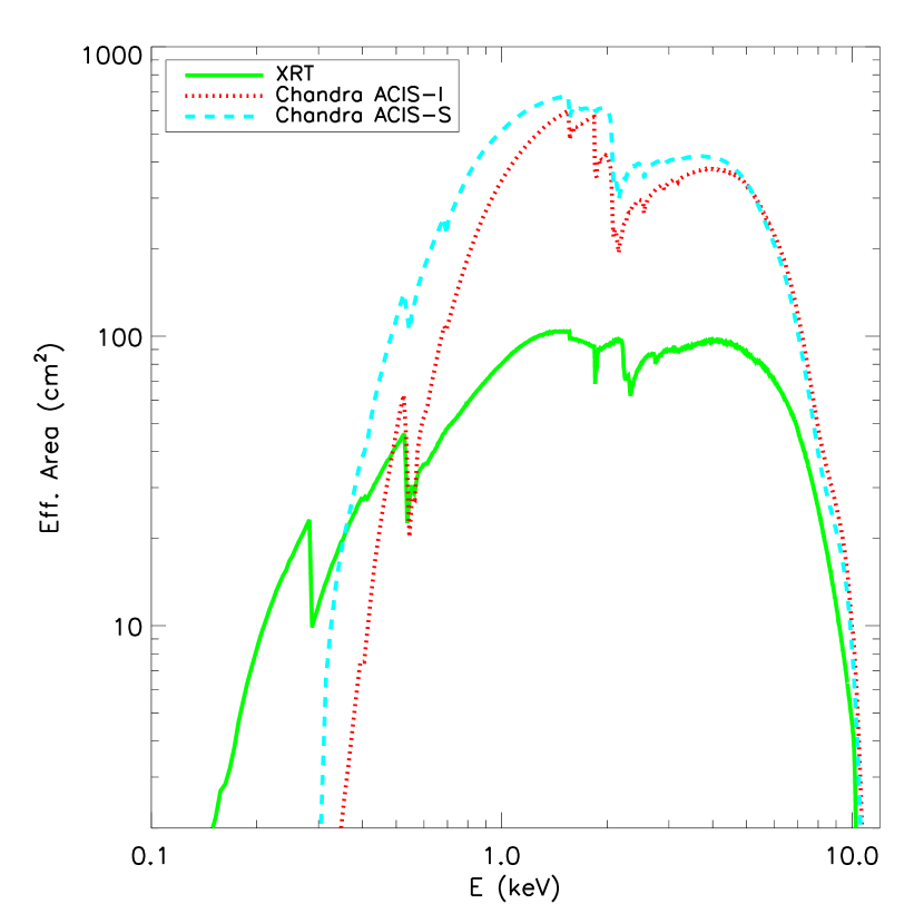
Figure 1: Effective area of XRT (green solid line) as a function of the energy compared with that of the Chandra satellite (red dotted and cyan dashed lines for Chandra ACIS-S and ACIS-I, respectively).

The catalog of extended sources presented in this paper constitutes the Swift X–ray Cluster Survey (SXCS) and it is based on the 336 GRB fields with galaxtic latitude $|b|>$20^∘ present in the XRT archive as of April 2010. The sources are identified thanks to a very simple but effective algorithm to select extended X–ray sources in the XRT soft band images. In this paper we adopt a conservative detection threshold which guarantees very low contamination and a well defined completeness function. This catalog is complementary to the catalog of point sources identified in the GRB fields of XRT by Puccetti et al. (2011), which focus on the study of the AGN population.

The paper is organized as follows. In § 2 we provide a description of the principal characteristics of the XRT. In § 3 we describe the field selection and the data reduction. In § 4 we describe the detection algorithm and the selection of the extended source candidates. In § 5 we describe how we performed extended source photometry. In § 6 we present the final list of groups and clusters in our sample, compute the sky coverage and the LogN–LogS, and check for possible selection bias. In § 7 we correlate our catalog with existing databases to identify previously known sources and collect the spectroscopic or photometric redshifts of member galaxies available in the literature. In § 8 we discuss our results in the context of current and future X–ray surveys. Finally, in § 9 we summarize our conclusions.

2 XRT characteristics

The XRT is part of the scientific payload of the Swift satellite (Gehrels et al. 2004), a mission dedicated to the study of gamma-ray bursts (GRBs) and their afterglows operating since January 2005. GRBs are detected and localized by the Burst Alert Telescope (BAT, Barthelmy et al. 2005), in the 15-300 keV energy band and followed–up at X–ray energies (0.3–10 keV) by the X–ray Telescope. The XRT (Burrows et al. 2005) is an X–ray CCD imaging spectrometer which utilizes the third flight mirror module originally developed for the JET-X program (Citterio et al. 1994). The mirror module focuses X–rays (0.2–10 keV) onto a XMM-Newton/EPICMOS CCD detector consisting of $600\times 600$ pixels, with a nominal plate scale of 2.36 arcseconds per pixel, which provides an effective FOV of the system of $\sim 24$ arcmin. The PSF, similar to XMM-Newton, is characterized by an half energy width (HEW) of $\sim 18$ arcsec at 1.5 keV Moretti et al. (2007). The PSF dependence on the off-axis angle is very weak. This is due to the fact that the CCD is intentionally slightly offset along the optical axis from the best on-axis focus in order to have a uniform PSF over a large fraction of the FOV, with a negligible dependence on the photon energy. To show the remarkably flat behaviour of the PSF, we show in Figure 2 the measured Half Power Radius (HPR) within a box of $45\times 45$ arcsec as a function of the off-axis angle for all the sources detected in the XRT fields used in this work. The PSF can be analytically described by a King function with slope $\beta\sim 1.45$ and core radius $r_{c}\sim 5.3$ arcsec (Moretti et al. 2007).

Figure 2: Measured HPR within a box of $45\times 45$ arcsec as a function of the off-axis angle for all the sources detected in the XRT fields used in this work.

One of the most relevant aspect for our purposes is the low level and the high reproducibility of the background not associated to astronomical sources (NXB). Due to the low orbit and short focal length, the NXB is the lowest among the currently operating X–ray telescopes (see Hall et al. 2007). As a reference, the NXB of XRT calculated per solid angle and normalized by the effective area is a factor $\sim 7$ lower than Chandra in the 0.5-7.0 keV energy band (Moretti et al. 2012 in preparation).

3 Fields selection and data reduction

We consider the entire Swift/XRT archive from February 2005 to April 2010, including 502 fields in the corresponding GRB positions, distributed in the sky as shown in Figure 3. We select the fields with Galactic latitude $|b|>$20^∘, to avoid crowded fields and strong Galactic absorption. This selection provides us with 336 fields which we use to search for extended sources.

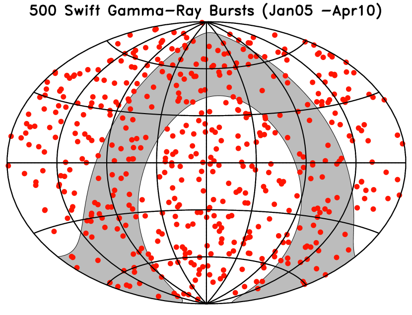
Figure 3: Distribution on the sky (Aitoff projection) of the GRB fields in the XRT archive as of April 2010 (red dots). The fields selected in our survey are those outside the Galactic plane (shaded area).

In this paper we use photon counting mode data with the standard grade selection (grade 0-12) reduced by means of the xrtpipeline task of the current release of the HEADAS software (version v6.8) with the most updated calibration at the time of writing (CALDB version 20111031, Nov 2011). More detail on the standard data reduction can be found in the instrument user guide. Then, we proceed with a customized data reduction, aimed at optimizing our data to the detection of extended sources. First we exclude the external CCD columns (corresponding to the detector coordinates Detx $<$ 90 and Detx $>$ 510) which are affected by the presence of out-of-time-events from corner calibration sources (see Moretti et al. 2009, for a detailed map of the CCD and a discussion on the XRT background). The corrected FOV, after removal of the external CCD columns, is 16.5$\arcmin\leavevmode\nobreak\ \times\leavevmode\nobreak\$18.9$\arcmin$ (0.087 deg²) for each pointing. Different observations of the same object and corresponding exposure maps are merged by means of the the extractor and farith tasks of the HEADAS software, respectively.

In order to further reduce the background, we investigate the background light curves in the soft image of each field. At the beginning of each observation, corresponding to the maximum emission from the GRB, the background on the entire image is significantly larger than the typical, quiescent value. Actually it was previosly known (Moretti et al. 2009) that for very high fluences, about 5% of the GRB X–ray emission is scattered across the image.

We effectively tested that by removing all the data taken before the epoch $T_{0}+0.1\times t_{exp}$, where $T_{0}$ is the epoch of the beginning of the observation, and $t_{exp}$ is the total effective exposure time, the average background on a typical image can be reduced by $\sim 5$%. This empiric rule is motivated by the fact that the total exposure time of a typical GRB follow–up observation is set by the GRB emission itself, therefore brighter GRBs will have larger observation length and therefore larger time intervals removed. In addition, note that the time interval $0.1\times t_{exp}$ does not correspond to 10% of the exposure time, since this is distributed over several orbits, each one with an observability time of 1500 s over a total orbit period of 5400 s. Figure 4 shows an example of a typical light curve, where the time interval that has been removed is shown in grey. The removal of the data up to the time $T_{0}+0.1\times t_{exp}$ corresponds typically to the first two or three orbits. On average, the time interval $0.1\times t_{exp}$ corresponds to 2-3% of the effective exposure time, since this is distributed over several days with 10-20 ks observed every day. We also note that removing the first orbits has the effect of reducing the non–homogeneity of the background caused by the GRB emission, which would have affected the detection of extended sources. In Figure 5 we show the distribution of the effective exposure times of the XRT fields after this correction.

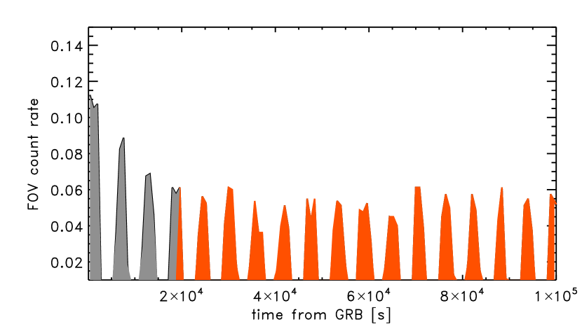
Figure 4: Light curve of the background of the field of GRB051008 plotted as a function of the time elapsed from the GRB trigger. The saw-tooth appearance is due to the orbits of Swift (one orbit lasts 90 minutes). The removed time interval below the epoch $T_{0}+0.1\times t_{exp}$ is shown in grey.

Figure 5: Distribution of the exposure times in ks for the 336 selected GRB fields.

4 Selection of extended-source candidates

4.1 Initial source detection

The identification of the X–ray sources is performed with the standard algorithm wavdetect within the CIAO software used successfully on Chandra and XMM-Newton images (Lloyd-Davies et al. 2011). We run the algorithm on the images obtained in the soft ($0.5-2$ keV) band using a set of six wavelet scales corresponding to 2, 4, 8, 16 and 32 image pixels. We use a mild selection threshold corresponding to the wavdetect threshold parameter $10^{-6}$. Despite not guaranteeing a high completeness nor high purity, this choice is motivated by the fact that the selection of extended sources will be based on the growth curve method, and that only relatively high S/N sources will be selected as we will show in Section 4.5. Therefore the wavdetect threshold parameter has no effects on our final cluster candidates list.

The soft band is optimal to identify extended ICM emission, since in this band XRT has the highest effective area and the lowest instrumental background. In this way we maximise our sensitivity in the detection of extended source powered by thermal bremsstrahlung, whose soft band emission has a small K-correction up to $z\sim 1$, at least for hot clusters (kT$>$3 keV). We also considered modifications to the standard soft band in order to find the energy range optimal for cluster detection, similarly to what has been done for Chandra and XMM–Newton (Scharf 2002). We explored the use of a narrower energy band in order to reduce the effect of the Galactic background, which rapidly grows below 1 keV. We found that a narrower energy band would have a minor positive effect on the detection of clusters, while negatively affecting the detection of low temperature groups whose emission is below 2 keV. We also explored the use of a larger upper energy value, but the poor photons statistics for thermal spectra at high energies and the rapidly increasing hard background nullify any advantage for values above 2 keV. Since the small, positive effects we found in changing the energy band are also significantly dependent on the temperature of the ICM, we decide to maintain the standard $0.5-2$ keV band.

Incidentally, we notice that, given the sensitivity at high energies of the XRT, it is possible in principle to use also the hard band (2-7 keV) to disentangle thermal emission from power-law emission typical of Active Galactic Nuclei (AGN), on the basis of the source hardness ratio. The hardness ratio is defined as HR=(H-S)/(H+S), where H and S are the hard band and soft band counts respectively, corrected for vignetting. In Figure 6 we show the hardness ratio as a function of redshift expected for groups and clusters at different temperatures, compared to the hardness ratio of AGN with different intrinsic absorption N_H. Values for clusters and AGN are taken using Xspec v12.6.0 assuming in the first case an absorbed thermal model with a mean Galactic absorption of $N_{H}=3\times 10^{20}$ cm^-2, and in the second case assuming an absorbed power law with an intrinsic redshifted absorption. We find that only nearby, strongly absorbed AGN have hardness ratio values clearly different from those of the ICM. We conclude that the hard band does not provide a relevant information for the detection of groups and clusters. Therefore we will use only the soft band in this work. The full band will be used for the spectral analysis of the brightest sources in a companion paper (Moretti et al. in preparation).

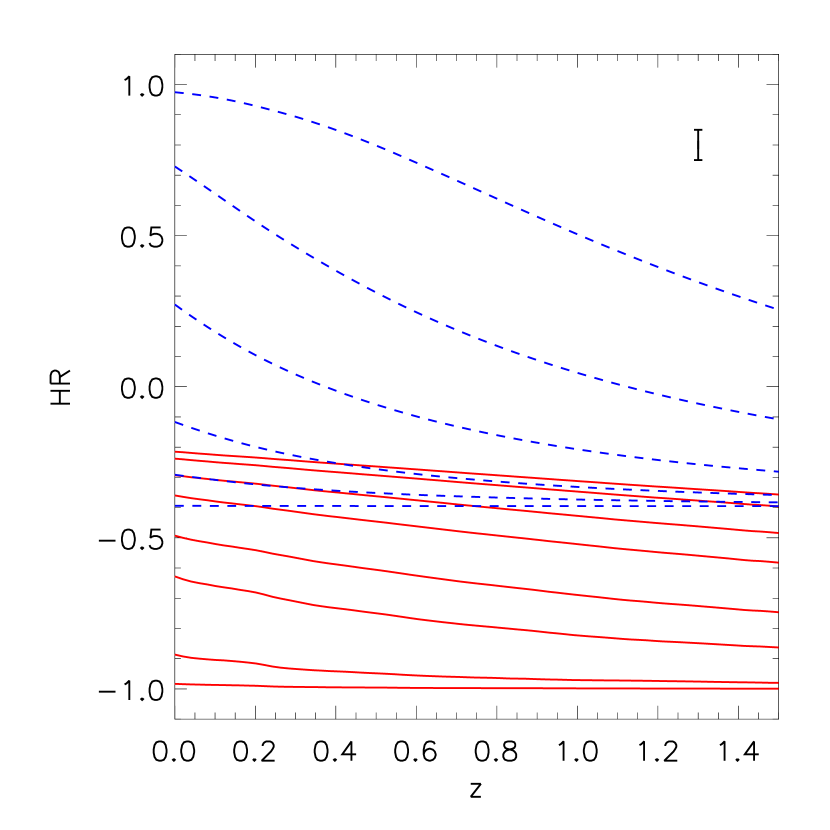
Figure 6: Hardness ratios modeled for XRT as a function of redshift for groups and clusters with several temperatures (red continuous lines, $kT$ respectively equal to 0.5, 1.0, 2.0, 3.0, 5.0, 7.0, 10.0 and 12.0 keV from the bottom to the top) and for AGN with different intrinsic absorption (blue dashed lines, N_H respectively equal to 0.01, 0.1, 0.3, 1.0, 3.0 and 10.0$\times$10²² cm^-2 from the bottom to the top). In the top right, we show the typical error bar on HR for a source with 200 total net counts.

Since the algorithm wavdetect has never been tested thoroughly on XRT images, we cannot immediately associate an expected contamination level to the threshold value of $10^{-6}$. In any case, at this stage we are mostly interested in collecting all the possible extended-source candidates, while the contamination level will be estimated during our selection process. This step leads us to identify a total of $\sim 10^{4}$ sources in the 336 GRB fields. This number is somewhat lower than that expected on the basis of the Swift serendipitous survey (SwiftFT, see Puccetti et al. 2011) which was based on a $\sim 20$% smaller field selection. The lowest number of net photons in our total source list is as low as 5. Despite the low background, Poisson fluctuations may appear as spurious sources at such a low signal. However, we do not apply any filter to this parent list, since much more stringent thresholds will be applied when selecting extended sources, as described in the next subsection.

4.2 Source extent determination

For each source we consider a 60$\times$60 pixels box centered around the source. In each of these boxes, we mask the other sources whose emission can overlap with the central one, by removing a PSF image. The PSF is accurately fitted with a King profile normalized to each source photometry assuming a core radius of $r_{c}=5.3$ arcsec and a $\beta=1.45$. These values are valid at energies $\sim 1.5$ keV and have been recomputed in–flight by fitting the many high S/N sources observed by XRT, therefore updating the values in Moretti et al. (2005) and Moretti et al. (2007). This gives us a sub–image cleaned from point-like sources, with the considered source at its center. In order to account for defects due to missing columns or removed pixels in the CCD, we divide this image by the corresponding soft exposure map. Then, we compute the growth curve of the source within a box of 45$\times$45 arcsec. This region corresponds to 2.5 times the HEW (which is 18 arcsec) and includes 80% of the flux of a point source. From the growth curve within this region, we measure the HPR, effectively defined as the 50% encircled energy radius within a box of $45\times 45$ arcsec. Note that the HPR is smaller than the HEW, since it refers to only 80% of the total flux. The choice of a restricted regions is motivated by the need of sampling the growth curve with a good signal-to-noise ratio (S/N) for the majority of the sources in the initial list. This choice does not affect by any means the final total flux, which will be computed according to a different procedure as shown in the next subsections, and it is used only to classify extended versus unresolved sources.

4.3 Point source simulation, and determination of threshold parameters

Extensive simulations spanning all the parameter range found in the survey (in particular source fluxes and background levels) have been used to estimate the expected distribution of the HPR for point sources. The input flux distribution for unresolved sources is consistent with the number counts obtained by Puccetti et al. (2011) and with the deeper CDFS counts (Rosati et al. 2002b), while the fluxes for clusters are distributed according with the number counts obtained in the ROSAT Deep Cluster Survey Rosati et al. (2002a).

The distribution of the measured HPR in the simulations as a function of the source counts within the 45$\times$45 arcsec box is shown in Figure 7. The simulations (including only point sources) are used to define the threshold values HPR_th above which a source is inconsistent with being unresolved at the 99% level (see red line in Figure 7). This criterion is extremely simple and it does not depend on the off–axis angle $\theta$, thanks to the flat PSF. However, HPR_th is a function of the source counts measured within the 45$\times$45 arcsec box, in particular it increases significantly below 60 counts. Above this value, HPR_th ranges between 3 and 4 image pixels (equal to 7.1-9.4 arcsec for a pixel size of 2.36 arcsec). Instead of using a single HPR_th based on the entire simulation, we compute HPR_th for a set of different background values, finding a significant dependence which will be taken into account in the source selection. By directly applying this criterion, we expect to have a number of spurious sources equal to 1% of the total source number. We remark that the counts within the 45$\times$45 arcsec box can be much lower than the total net counts, particularly for extended sources.

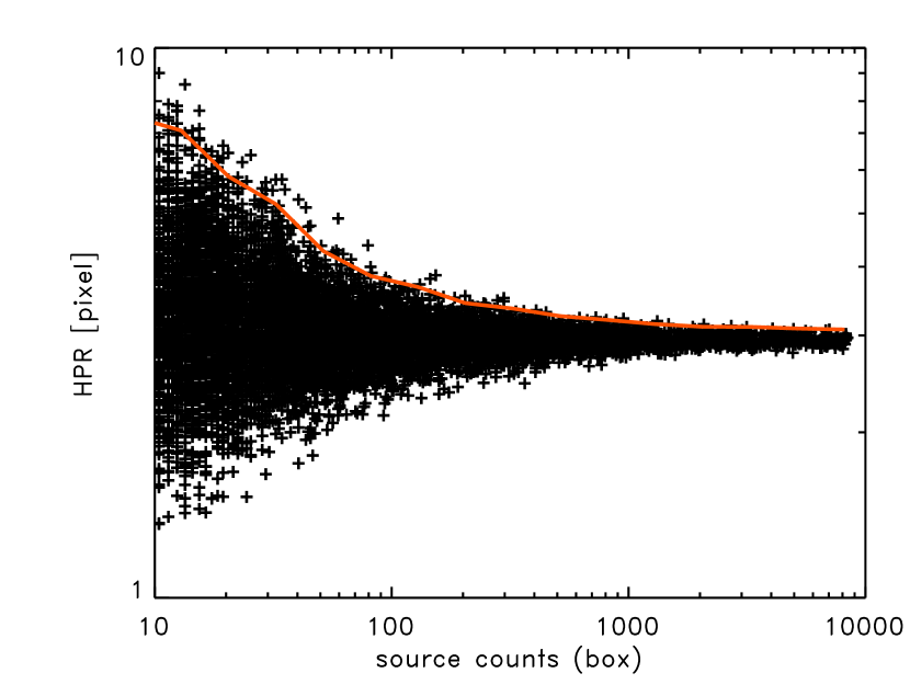
Figure 7: Distribution of the measured HPR within a 45$\times$45 arcsec box for simulated unresolved sources as a function of the soft counts within the box. The same range of exposure times and backgrounds present in the real data has been adopted in the simulations. The continuous line shows the 99% confidence level envelope of the source distribution.

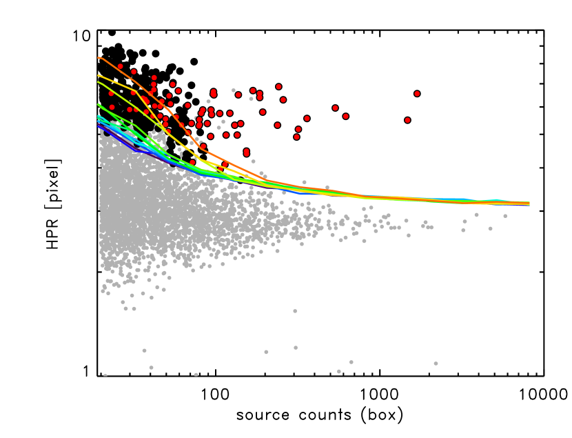
Figure 8: Distribution of the measured HPR within a box of $45\times 45$ arcsec for all the sources detected in the XRT fields as a function of the soft counts measured within the HPR. All possible extended source candidates are marked with black big dots, while red big dots indicate sources with $>$100 soft net counts from the aperture photometry in the extraction radius (see Section 5) and are therefore included in the cluster candidate list. The continuous lines show the typical 99% confidence level envelope for different exposures, from 1 ks (orange line) to 1 Ms (blue line).

This procedure is applied to all sources detected with wavdetect. Figure 8 shows the distribution of the HPR of the detected point sources (grey dots) versus the source counts measured inside the HPR, with the extended source candidates marked as black and red big dots. Note that extended source candidates are selected on the basis of a HPR_th value which depends also on the background (tied to the exposure of the image). The HPR_th for different exposures are shown in Figure 8 as solid lines ranging from 1 ks (orange line) to 1 Ms (blue line). The number of extended source candidates grows rapidly when the number of detected counts within the box decreases towards low values. The inclusion of all the candidates in our survey clearly would imply a large number of spurious sources, given the large total number of sources ($\sim 10^{4}$). We finally apply the threshold on the total number of counts to be $>100$ in the extraction radius (defined as the circular region where the source surface brightness is larger than the background level). The red big dots indicate the candidate extended sources matching all our selection thresholds.

The sharp threshold on the soft net counts allows us to compute directly a sky coverage as a function of the source flux within the extraction region (see Section 6). Clearly, the sky coverage information would be sufficient to compute the logN-logS only in absence of any morphology bias. Actually, we do miss a fraction of extended sources, mostly due to the wide range of intrinsic morphologies. The completeness of our survey is then estimated as described in the next subsection.

4.4 Completeness and contamination level

To properly characterize the quality of our sample we need to assess the completeness, defined as the fraction of extended sources actually selected as extended by our procedure as a function of their soft net counts. In order to estimate the completeness, we realize another set of simulations with a different strategy. We simulated a few thousand extended sources, spanning a wide range of fluxes consistent with the number counts measured in the ROSAT Deep Cluster Survey (Rosati et al. 1998).

Our extended sources are modelled starting from ten real cluster images originally obtained with the Chandra satellite (therefore with a resolution much higher that that of XRT), cloned at a typical redshift and resampled at the XRT resolution. This cloning procedure, already used to investigate the evolution of cool core clusters at high redshift (see Santos et al. 2008, 2010) allows us to measure our completeness for a realistic range of surface brightness profiles, representing the local population of groups and clusters of galaxies: temperatures go from 2 keV to 8 keV, the redshift of the clusters are all below 0.2, and half of the clusters have a cool core. Clearly, the limited set of group/cluster templates, and the assumption of no evolution in the surface brightness properties with redshift, may introduce some difference with respect to the actual cluster population. The impact of the intrinsic morphologies on the source selection is properly taken into account as long as the morphologies of the simulated sources are representative of the real sources. This is admittedly a limitation of the present approach. Still, this procedure is the most accurate with the present knowledge. The simulated clusters are positioned randomly on real XRT images and the fluxes are converted into count rate using the response function of the instrument, including vignetting effects. We run our detection procedure on the simulated images, and compute the completeness as the recovered source fraction (i.e., the fraction of sources detected and characterized as extended with our criterion) as a function of the input counts. As shown in Figure 9, we reach a completeness level $\sim$70% for sources above our threshold of $\sim$100 net counts within the extraction regions. This level increases to $\sim$90% for sources with $\sim$200 net counts, and reach a completeness level of $>$95% for sources with $\sim$300 net counts. We will use this information to correct the logN-logS of our sample in § 6. We remark that this completeness function is by no means general: it depends, in fact, on the intrinsic properties of the survey, on the exposure time distribution, and on the source selection and classification method. We are actually aiming at increasing the completeness down to a threshold of $\sim$50 net counts, while maintaining a low contamination level, thanks to a different detection algorithm based on Voronoi tessellation (Liu et al. in preparation).

Finally, our simulations allow us to estimate also the contamination level. This is obtained directly by averaging the number of spurious sources surviving our selection criteria in all our survey realizations. The average expected number of spurious sources in the SXCS survey turns out to be $\sim 5$. The contamination is due to Poisson noise in the measured parameters (HPR, photometry) and to blending. We neglect any spatial correlation which, however, is expected to give a negligible enhancement to the contamination level.

4.5 Final sample selection

Our algorithm identified 87 candidate extended sources with $\geq$100 soft net counts. We proceeded to a careful visual inspection of these candidates, including a look through the optical images taken from the DSS and from the SDSS when available. This visual inspection allows us to remove 3 sources which are identified with stars. In addition, 3 sources are removed since they are identified with nearby large galaxies. Note that all these sources are correctly identified as extended by our algorithm.

We also remove 6 sources since they are easily recognized as blended by visual inspection. This effect was included in the simulations which predicted a number of spurious sources equal to 5. We argue that our visual inspection actually remove most of the spurious detections. The visual inspection is made possible thanks to the limited size of our sample. For larger samples, a more efficient, self-consistent detection algorithm would be needed in order to keep the contamination level under control down to lower fluxes, without recurring to time-consuming visual inspections.

Another 3 sources are found to be very close to the edge of the XRT images, where the gradient of the exposure map significantly affects the photometry. We remove them since their photometry would necessarily rely on a substantial extrapolation of their properties. The final sample includes 72 extended sources. Figure 10 shows a typical example of a GRB field imaged by XRT. In this case (GRB050505) three extended sources, highlighted by green circles, have been selected by our algorithm.

Figure 9: Completeness level, expressed as the ratio of recovered extended sources on the number of simulated extended sources as a function of the input soft counts.

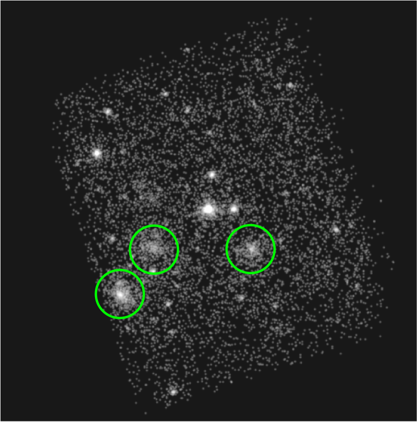
Figure 10: XRT smoothed image of the GRB050505 field in the soft ($0.5-2.0$ keV) band; the exposure time is $\sim$170 ks, and the image size is $\sim$24$\times$24 arcmin. The three clusters in the fields are highlighted by the green cicles. The bright source at the center is the GRB.

5 Extended sources photometry

The measured net counts from each source are computed by aperture photometry up to an extraction radius R_ext, after removing the emission associated to point sources included in this region. R_ext is defined as the radius where the surface brightness profile of the source reaches the background level. The total net counts are finally obtained by accounting for the missed flux beyond $R_{ext}$. In order to measure the lost signal, we fit the surface brightness SB of every extended source with a King profile modeled as SB$\propto(1+(r/r_{c})^{2})^{3\beta-1/2}$ (Cavaliere & Fusco-Femiano 1978) leaving both $r_{c}$ and $\beta$ free to vary. Then, we extend the surface brightness profile up to $2\times R_{ext}$. The typical ratio of the total estimated flux to that actually measured within $R_{ext}$ is $c_{f}=1.05-1.10$. Extrapolating the profile to larger radii has a modest effect on the final results. We also checked that the errors on the $r_{c}$ and $\beta$ parameters affect the correction factor $c_{f}$ only at a 10% level, and therefore constitute a negligible uncertainty for the final source flux.

The net count rate measured for each source is obtained dividing the net counts by the exposure time, after correcting for vignetting effects in the soft ($0.5-2$ keV) band. The average vignetting correction in the extraction region is estimated by the ratio of the photon-weighted average value of the soft exposure map within R_ext to the value of the soft exposure map at the aimpoint. From the corrected net count rate, the energy flux is computed simply by multiplying it by the energy conversion factor (ECF) computed at the aimpoint for a suitable spectral model.

The ECF for thermal X–ray emission from the ICM is computed assuming a mekal model within XSPEC. Since we do not know a priori the temperature of our sources, we explore a range of temperatures from 1 to 12 keV, and a redshift range from 0 to 1.5. The corresponding ECF values in the soft band are shown in Figure 11 for a typical Fe abundance of 0.3 $Z_{\odot}$ in units of Anders & Grevesse (1989). We note that the ECFs vary less than 2% for kT$>$3 keV at any redshift. The largest changes are found for lower temperatures, up to a maximum of 8% for kT$=$1 keV. However, given the average $L-T$ relation measured locally, and considering that it is approximately constant with redshift (Reichert et al. 2011; Branchesi et al. 2007; Maughan et al. 2006; Ettori et al. 2004; Mushotzky & Scharf 1997), we can derive a minimum temperature detectable at a given redshift for our flux limit. If we set $F_{lim}\sim 10^{-14}$ erg s^-1 cm^-2, we find that clusters and groups with kT$<$2 keV can be observed only for $z<$0.5. This allows us to conclude that the maximum variation is below 4%, and that this number is little affected by the actual ICM metallicity. Therefore we assume an average ECF of $2.35\times 10^{-11}$ erg s^-1 cm^-2/ (cts s^-1) with a maximum systematic uncertainty of $0.1\times 10^{-11}$ erg s^-1 cm^-2/ (cts s^-1).

The ECFs, however, have a more significant dependence on the Galactic absorption. This can be estimated thanks to the Galactic N_H values measured in the radio survey in the Leiden/Argentine/Bonn survey (Kalberla et al. 2005). As shown by the histogram in Figure 12, the distribution of Galactic N_H for our sources implies changes up to the order of 30%. Therefore we use for each detected source the ECF appropriate to the corresponding field. We note that self shielding of molecular Hydrogen from ambient UV radiation is expected to occur for $N_{H}>5\times 10^{20}$ cm^-2 (Arabadjis & Bregman 1999), and this molecular gas absorbs also X–rays. Therefore for this $N_{H}$ values X–ray fluxes are slightly underestimated. We do not correct for this effect (see also Lloyd-Davies et al. 2011).

To summarize, the total unabsorbed, soft fluxes, including the correction up to 2 $R_{ext}$, are measured as:

$$S_{0.5-2keV}=ECF(N_{H})\times c_{f}\times C_{rate}$$ (1)

where $ECF(N_{H})$ is the energy conversion factor which accounts for the Galactic absorption (see Figure 12), $c_{f}$ is the correction factor for the flux between $2\times R_{ext}$ and $R_{ext}$, and $C_{rate}$ is the soft band count rate mesured within $R_{ext}$ and corrected for vignetting effects.

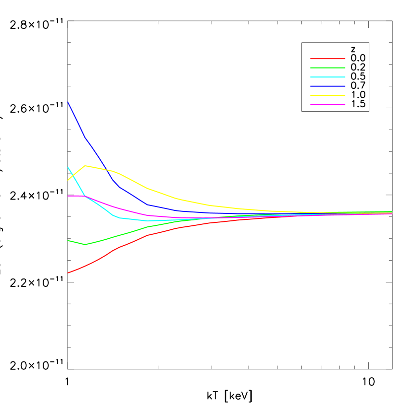
Figure 11: Energy Conversion Factor (ECF) as a function of the ICM temperature for different redshifts. Here we assumed no Galactic absorption.

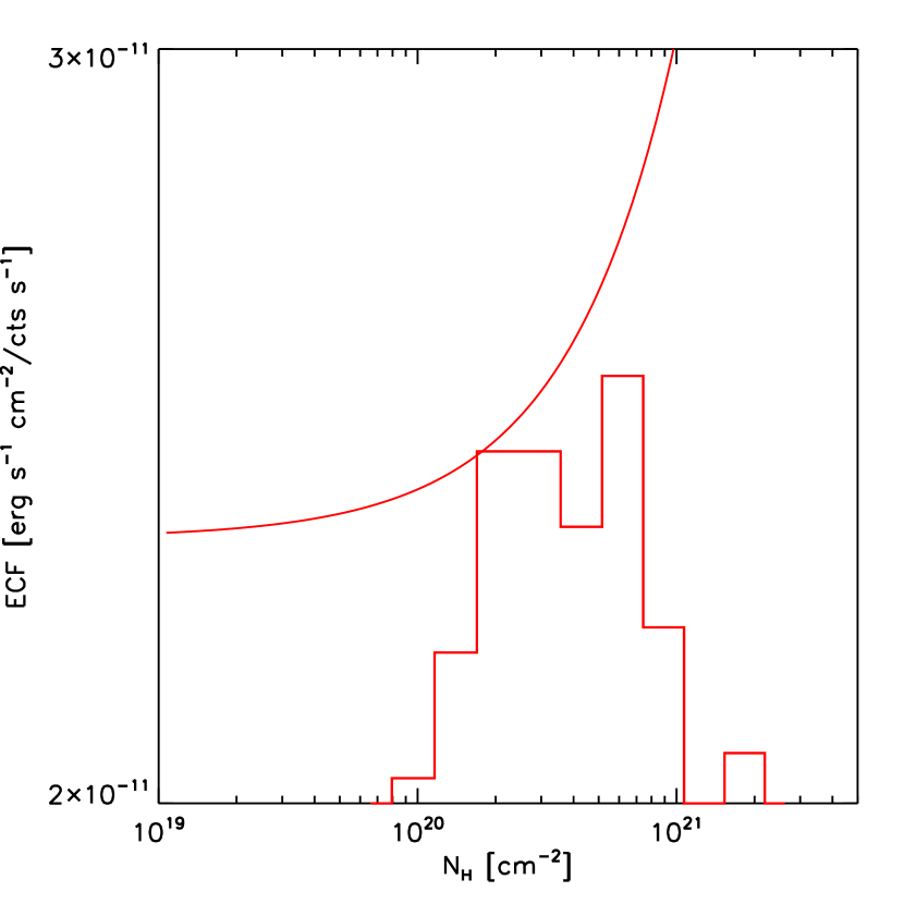
Figure 12: Energy Conversion Factor (ECF) as a function of the Galactic N_H for a typical cluster (kT$=$5 keV, $z=$0.4). The histogram shows the distribution of Galactic N_H in our cluster sample.

6 Cluster catalog and Number Counts

Aperture photometry within $R_{ext}$ and total energy flux are shown in Table LABEL:table2 for all the sources of our sample. The net counts error is obtained from the Poissonian error on the numbers of net photons. We remark that, as explained in detail in the previous section, the photometry of our extended sources refers to the extraction radius R_ext defined as the radius where the fitted surface brightness falls below the measured local background, while the total energy flux include the correction factor $c_{f}$ for the flux lost beyond R_ext.

In order to compute the number counts for our cluster sample, we need to derive the sky coverage of our survey. The sky coverage is determined by the sharp limit in the total net photons. For each field we compute a flux-limit map obtained as $ECF(N_{H})\times 100/Expmap(t)$, where $Expmap(t)$ is the exposure map in units of effective time, therefore including the effect of vignetting. Then, the solid angle covered by the survey above a given flux is obtained by measuring the total solid angle where the flux-limit is lower than a given flux. In Figure 13 we show the resulting sky coverage $\Omega(S)$ and compare it with the sky coverage of the 400 Square Degree ROSAT PSPC Galaxy Cluster Survey by Burenin et al. (2007) and with the sky coverage of the ROSAT Deep Cluster Survey (RDCS) by Rosati et al. (1998). Unfortunately, sky coverage curves for other on-going XMM/Chandra surveys have not been published. The cumulative number counts for sources brighter than a given flux S is therefore given by

$$N(>S)=\Sigma_{c_{f}\times S_{i}>S}C_{i}^{-1}/\Omega(S_{i})$$ (2)

where $S$ is the total flux, $S_{i}$ is the soft flux within $R_{ext}$ of the $i^{th}$ source, $c_{f}$ is the correction factor for the flux outside $R_{ext}$ and $\Omega(S_{i})$ is the solid angle corresponding to $S_{i}$. Finally, $C_{i}$ is the completeness factor plotted in Figure 9 which depends on the net detected photons of the $i^{th}$ source. In this way, each source is weighted with a factor inversely proportional to the survey completeness which depends only on source photometry.

An alternative procedure to correct for completeness is obtained by randomly extracting the missing sources and computing their average effect. The procedure consists in dividing the sources in 3 bins of net photons (100-150, 150-200, 200-300). Then, in each bin we randomly add a number of sources drawn from a Poissonian distribution centered on the expected number of missed sources according to Figure 9. Finally we assign a random exposure and energy conversion factor among those in the survey to each mock source, and compute its energy flux. Finally the logN-logS is recomputed for each Monte Carlo realization. The average logN-logS obtained with this procedure with $10^{4}$ realizations is in very good agreement with that obtained with equation 2, therefore confirming that our treatment of the completeness is robust.

Our logN-logS is shown in Figure 14 with its 68% confidence limits (shaded red region). The confidence limits are computed with Monte Carlo realizations. We re-extract the flux of each source times assuming its Poissonian uncertainties on the net detected counts, including the systematic uncertanty on the ECFs, obtaining $10^{4}$ realizations of the logN-logS. Then, at each flux, we compute the 68% confidence interval around the mean value.

Our results are consistent with the logN-logS measured with the ROSAT Deep Cluster Survey (RDCS, Rosati et al. 1998), shown in Figure 14 as the cyan region, down to fluxes $\sim 10^{-14}$ erg s^-1 cm^-2. We are also consistent with the the logN-logS measured in the 400 deg² survey (Burenin et al. 2007) and in the COSMOS field (Finoguenov et al. 2007), shown as the dash-dotted and dotted lines respectively.

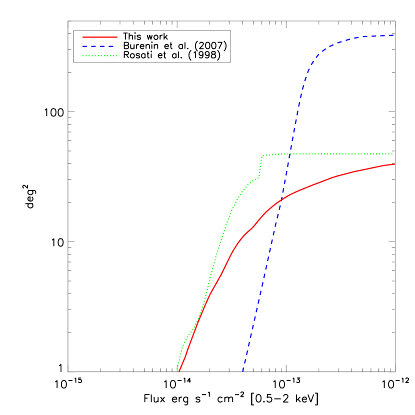
Figure 13: Solid angle $\Omega$ covered by our survey as a function of the soft flux. As a comparison, we show also the sky coverage of the 400 Square Degree Survey (Burenin et al. 2007, blue dashed line) and the sky coverage of the RDCS (Rosati et al. 1998, green dotted line).

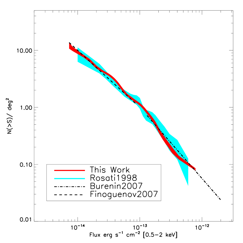
Figure 14: Cumulative number counts, corrected for completeness, with 1 $\sigma$ confidence level for SXCS (red area), compared to the logN–logS derived from the ROSAT Deep Cluster Survey (cyan area), Rosati et al. (1998). Dot-dashed and dashed lines show the fit to the 400d (Burenin et al. 2007) and to the COSMOS (Finoguenov et al. 2007) number counts, respectively.

Figure 15: Positions of our sources with respect to the GRB position (set to 0,0).

The good agreement with previous results confirm the proper characterization of our sample. Nevertheless, we also perform a test against a possible correlation between the GRB position and the position of our sources, since the detection of an enhanced density of clusters and groups toward the position of GRB would bias our survey. In Figure 15 we plot the positions of the sources in our sample with respect to the GRB positions (set to 0,0). We do not find any hint of an increasing surface density of extended sources towards the GRB position. We also tested for such a possible bias by measuring the logN-logS for the sources whose distance is, respectively, below 400 arcseconds from the GRB and between 400 and 800 arcseconds from the GRB. The two logN-logS agree with each other within the uncertainties, showing that there is no correlation between GRB and clusters (see also Berger et al. 2007). We can safely assume that our field selection is unbiased with respect to X–ray clusters.

In order to check whether we properly treated the effect of the Galactic absorption, we split the survey into two segments according to the Galactic absorption, above and below $N_{H}=3\times 10^{20}$ cm^-2. We find that the logN-logS computed in the two cases are in very good agreement, and therefore we conclude that our flux measurements do not appear to suffer any bias from Galactic absorption.

To summarize, the sources included in the SXCS catalog represent a sample of group and cluster candidates with a negligible contamination, a well defined selection function and a robustly estimated completeness, spanning two orders of magnitude in flux, and reaching the flux limit of $\sim 10^{-14}$ erg s^-1 cm^-2.

7 Cross-correlation with X–ray and optical catalogs.

We checked for counterparts both in previous X–ray surveys and in optical cluster surveys, assuming a search radius of 1 arcmin from our X–ray centroid. The results are shown in Table 3. We find 9 X–ray counterparts to our sources in ROSAT, ASCA and Chandra catalogs, none of them characterized as extended and none of them with a published redshift. We also find a total of 20 previously known, optically identified clusters. Among them, 6 are found in the Wen+Han+Liu cluster sample (WHL, Wen et al. 2009), which is an optical catalog of galaxy clusters obtained from an adaptive–matched filter finder applied to Sloan Digital Sky Survey DR6. We find 4 clusters in the Szabo et al. (2011) catalog (AMF) based on a similar method in the SDSS DR6.

We also report one cluster from the Gaussian Mixture Brightest Cluster Galaxy (GMBCG, Hao et al. 2010) based on SDSS DR7, which is an extension of the maxBCG cluster catalog (Koester et al. 2007) to redshift beyond 0.3 and on a slightly larger sky area ($\sim 8000$ deg²), and one cluster in the MaxBCG catalog itself.

Finally, we find 3 clusters in the Abell catalog (Abell et al. 1989), two cluster in the Northern Sky optical Cluster Survey (NSCS, Gal et al. 2003; Lopes et al. 2004), and one cluster in each of the following catalogs: the Zwicky Cluster Catalog (CGCG, Zwicky et al. 1963), the Sloan Digital Sky Survey C4 Cluster Catalog (SDSS-C4-DR3, based on DR3, Miller et al. 2005; von der Linden et al. 2007), the Edinburgh-Durham Southern Galaxy Catalogue (EDCC, Lumsden et al. 1992). Three out of twenty clusters also have an X–ray counterpart.

To increase the number of available redshifts, we also search for galaxies with published redshift not associated to previously known clusters, within a search radius of 7 arcsec from the X–ray centroid of our sources. In Table 3 we report 11 galaxies with redshift, within a search radius of 7 arcsec, as a complement to the redshift of the cluster counterpart. The redshift of the central galaxy candidate is always consistent with the photometric redshift of the optical cluster counterpart when present. In the 4 cases where no optical cluster counterpart is found, we tentatively assign the galaxy redshift to our X–ray source. We note that both cluster and central galaxy counterparts have been found by adopting a simple matching criterion. A more refined analysis of the optical data covering our survey is under way (Tundo et al. in preparation).

To summarize, we have 24 optical redshifts (spectroscopic or photometric) published in the literature and associated to our cluster candidates. Overall, 46 sources in our catalog are new detections, both as X–ray sources and as clusters of galaxies. Finally, we remark that a total of 32 SXCS sources fall in SDSS fields. Thanks to the SDSS depth, we expect to increase the identification of our cluster candidates. In particular we expect to be able to identify at least the brightest cluster galaxy up to $z\leq 1$ for those cluster candidates which are not already included in the SDSS catalogs. This will also provide an estimate of the photometric redshift of the host cluster. Figure 16 shows a selection of SDSS r-band images of SXCS fields, with X–ray contours overlaid in green.

We stress that we can also attempt a measure of the source redshift through the X–ray spectral analysis for a significant fraction of the sample. The requirements for a successfull identification of the redshifted $K_{\alpha}$ Fe line, shown in Yu et al. (2011) for Chandra, do not apply to most of the SXCS sources. However the lower background and the flatter effective area of XRT may allow X–ray redshift measurements in a lower S/N regime. A preliminary result indicates that the X–ray redshift $z_{X}$ of about 30% of the SXCS sources can be successfully measured. This is an important aspect since the measure of $z_{X}$ will complement the photometric and spectroscopic redshifts obtained with optical follow–up with the aim of using the cluster sample for cosmological tests. We will present the spectral analysis in a companion paper (Moretti et al. in preparation).

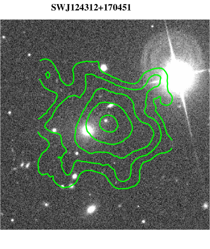
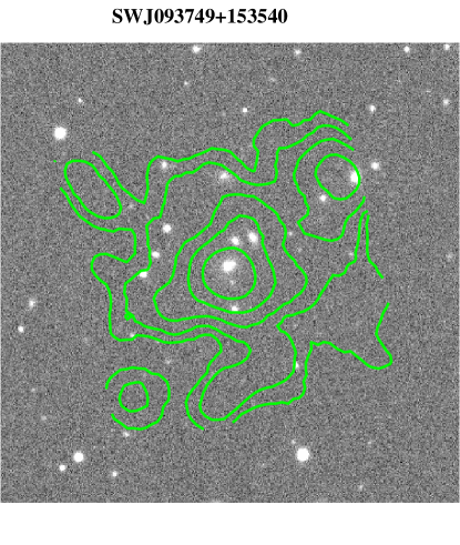
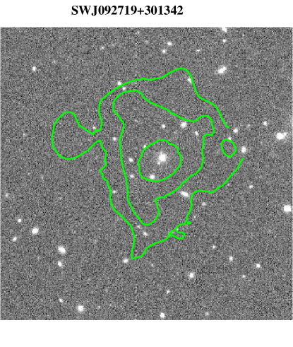
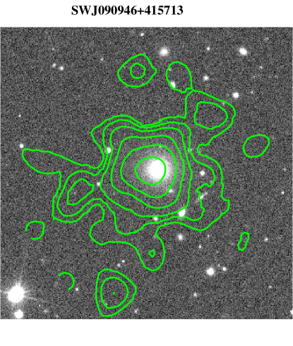
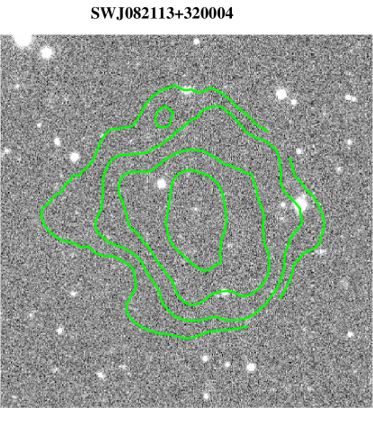
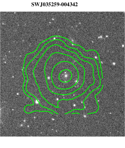
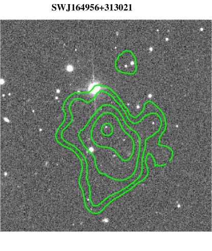
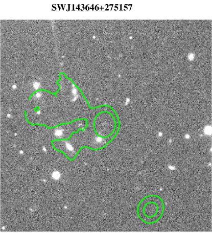
Figure 16: Selection of SXCS cluster candidates imaged by the Sloan Digital Sky Survey (SDSS) with X–ray contours overlaid in green. The image size is 3$\times$3 arcmin. The X–ray contours are computed on XRT images in the $0.5-2$ keV energy band with the Chandra Ciao software, and the contours are drawn at respectively 9, 15, 30, 50, 90, 160 and 300 $\sigma$, where $\sigma$ is given by the local background level.

8 Future prospects

SXCS data have different properties from Chandra and XMM–Newton data as described in § 2 and § 3, and therefore SXCS extended sources have a different selection function. For these reasons the SXCS is a valuable touchstone to the cluster catalogs obtained from XMM-Newton and Chandra. The full SXCS survey (Liu et al. in preparation) is expected to cover a larger solid angle especially at bright fluxes, and to be at least a factor of two deeper. The exploitation of the Chandra and XMM archives is still far from being concluded, and we expect to see the number of high–$z$ clusters ($z>1$) to double in the next years, and in particular to see the increase of the sample of clusters at $z>1.5$ which are being found only recently. However, a major breakthrough in the field of cluster surveys can be achieved only with a survey dedicated mission.

The planned eROSITA satellite (Predehl et al. 2010; Cappelluti et al. 2010) and the proposed WFXT mission (Rosati et al. 2010; Murray et al. 2010) can provide a large number of new detections and X–ray spectra for a large number of them. The eROSITA mission is expected fo fly in the near future, and it will finally provide an all-sky survey almost two orders of magnitude deeper than the last one performed by the ROSAT satellite (Voges et al. 1999), filling a gap of almost 20 years. Unfortunately, eROSITA will be confusion limited in the flux regime where the majority of the high–$z$ clusters are expected. In addition, the low hard–band sensitivity (the effective area decreases an order of magnitude from 1 keV to 4 keV) hampers a measure of the temperature for hot clusters, limiting cosmological studies.

The WFXT is the only X–ray mission optimized for efficient wide-area surveys, with a design which yields good angular resolution and a constant image quality across a large (1 deg²) field of view (see Rosati et al. 2010). These aspects, coupled with a large effective area, will provide not only a survey more than one order of magnitude deeper than eROSITA, but a direct measurement of global temperatures, density profiles and redshifts for a significant fraction of the cluster sample, thus allowing cosmological studies independently of optical and spectroscopic follow–up (Borgani et al. 2010). Simulations based on the original WFXT design (Tozzi et al. 2010) show that such a mission is able to match in depth, survey volume and angular resolution surveys at other wavelengths which are planned for the next decade.

9 Conclusions

We present a new sample of X–ray selected groups and clusters of galaxies obtained with the X–ray Telescope (XRT) on board of the Swift satellite. We search for extended sources among 336 GRB fields imaged with XRT with galactic latitude $|b|>$20^∘ (available in the archive as of April 2010). We identify extended sources with a simple criterion based on the measurement of the HPR within a box of $45\times 45$ arcsec of the source image. We apply a sharp threshold of 100 net soft counts within the extraction radius $R_{ext}$ to select reliable extended sources. Extensive simulations showed that our method, despite being very simple, provide us with an X–ray sample with an expected high completeness and a low contamination, also thanks to a careful a posteriori visual inspection.

Our final group and cluster catalog consists of 72 X–ray sources. The sky coverage of the survey goes from the total 40 deg² to 1 deg² at a flux limit of about $10^{-14}$ erg s^-1 cm^-2. The corresponding logN–logS is in very good agreement with previous deep surveys.

We directly verified that there is no correlation between the position of the clusters and that of the GRBs. In other words, selecting our cluster sample from XRT GRB fields does not result in any spatial bias with respect to the GRB positions.

A cross correlation with X–ray catalogs shows that only 9 SXCS sources were previously identified in the X–ray band, none of them classified as extended. A search in optical databases (mostly based on SDSS data) allows us to find the counterparts of 20 clusters. In addition, 4 galaxies with redshift have been found to be within 7 arcsec from the X–ray centroid, and therefore they are considered as possible identification of the central galaxy of the group/cluster candidate. Overall, only 20 sources are confirmed as clusters using data from the literature, while 30 sources have some counterpart in the NASA Extragalactic Database, and, finally, 42 sources are newly identified.

We estimate that about one third of the sample is detected with a S/N high enough to allow the measure of the redshift from the X–ray spectral analysis (see Yu et al. 2011), as we will show in a companion paper (Moretti et al. in preparation). Thanks to the quality of our X–ray data, and thanks to the synergy with other surveys, specifically the SDSS, we are able to provide a X–ray cluster sample with a well established completeness function down to a flux limit comparable to that of the deepest cluster surveys based on ROSAT data (RDCS, see Rosati et al. 1998), and with a comparable statistics. In addition, we expect to detect a few clusters with redshift $z\geq$1. Overall, the SXCS is expected to give a significant contribution in the field of X–ray clusters surveys also thanks to its peculiar properties of a low background and a constant PSF. These properties are two key requirements for future wide–area, X–ray surveys, as foreseen by proposed future missions aiming at bringing the X–ray sky to the same depth and richness of the optical and IR sky in the next decade. A deeper, extended release of the SXCS based on a new detection algorithm tailored to XRT images is currently undergoing (Liu et al. in preparation). Catalog and data products of SXCS, constantly updated, are made avalilable to the public through the website http://adlibitum.oats.inaf.it/sxcs.

2

Table 2: SXCS sources.

Name	ra	dec	Exptime	NH	Rext	Soft Cts	Soft SNR	Soft Flux
	deg		[s]	$10^{20}$ cm-2	arcsec			10-14erg s-1 cm2
SWJ000345-530149	0.93793	-53.03028	301809	1.60	18	191$\pm$ 17	10.8	1.6$\pm$ 0.2
SWJ000315-525510	0.81655	-52.91970	303488	1.60	44	1487$\pm$ 46	31.9	12.0$\pm$ 1.3
SWJ000324-525350	0.85004	-52.89743	289366	1.60	52	1847$\pm$ 52	35.2	15.7$\pm$ 1.9
SWJ002437-580353	6.15751	-58.06475	74764	1.22	43	315$\pm$ 20	15.5	10.3$\pm$ 1.2
SWJ003316+193922	8.31936	19.65637	44186	4.14	41	126$\pm$ 13	9.4	7.5$\pm$ 1.1
SWJ005500-385226	13.75198	-38.87410	40951	3.32	36	104$\pm$ 12	8.3	6.6$\pm$ 1.0
SWJ011432-482824	18.63735	-48.47342	38003	1.95	47	158$\pm$ 15	10.5	10.3$\pm$ 1.4
SWJ012210-130422	20.54544	-13.07302	62075	2.35	28	101$\pm$ 12	8.3	4.1$\pm$ 0.7
SWJ012302+375615	20.76171	37.93769	75637	6.03	31	120$\pm$ 12	9.3	4.4$\pm$ 0.7
SWJ015753+165933	29.47116	16.99270	77327	4.85	27	104$\pm$ 11	8.8	3.6$\pm$ 0.6
SWJ020744+002055	31.93682	0.34872	83492	2.34	24	119$\pm$ 12	9.7	3.6$\pm$ 0.5
SWJ021705-501409	34.27108	-50.23602	131772	1.80	44	749$\pm$ 30	24.4	14.0$\pm$ 1.6
SWJ021747-500322	34.44821	-50.05631	122374	1.80	29	207$\pm$ 16	12.3	4.2$\pm$ 0.6
SWJ022344+382311	35.93546	38.38647	150608	4.40	13	102$\pm$ 11	9.2	1.8$\pm$ 0.3
SWJ022546-185553	36.44202	-18.93140	403267	2.81	37	813$\pm$ 33	24.3	5.1$\pm$ 0.6
SWJ023224-712020	38.10299	-71.33891	316584	5.79	19	212$\pm$ 17	11.9	1.8$\pm$ 0.2
SWJ023302-711634	38.26142	-71.27616	323540	5.79	43	1284$\pm$ 42	30.2	10.8$\pm$ 1.2
SWJ023924-250504	39.85054	-25.08445	118554	2.23	38	323$\pm$ 21	15.3	6.8$\pm$ 0.9
SWJ024010-251121	40.04202	-25.18923	242137	2.23	19	115$\pm$ 13	8.5	1.2$\pm$ 0.2
SWJ035259-004342	58.24825	-0.72847	107623	11.30	44	1461$\pm$ 40	36.3	42.2$\pm$ 4.4
SWJ035310+213335	58.29573	21.55977	83256	11.30	32	137$\pm$ 14	9.8	5.1$\pm$ 0.8
SWJ044144-111536	70.43740	-11.26022	68676	4.61	36	311$\pm$ 19	15.7	12.0$\pm$ 1.5
SWJ062155-622834	95.48190	-62.47626	1039776	4.49	13	286$\pm$ 20	13.8	0.7$\pm$ 0.1
SWJ082113+320004	125.30467	32.00130	117078	3.35	35	597$\pm$ 27	22.0	13.1$\pm$ 1.4
SWJ083340+331102	128.41815	33.18397	32951	4.07	39	142$\pm$ 13	10.7	11.3$\pm$ 1.6
SWJ084749+133141	131.95442	13.52810	77386	3.18	54	3824$\pm$ 63	60.6	126.4$\pm$ 12.9
SWJ085524+110201	133.85220	11.03384	85418	3.54	33	204$\pm$ 16	12.4	6.2$\pm$ 0.8
SWJ090946+415713	137.44232	41.95386	12328	1.23	46	133$\pm$ 12	10.9	26.3$\pm$ 3.6
SWJ092619-090546	141.57982	-9.09634	46474	3.78	51	251$\pm$ 18	13.8	14.1$\pm$ 1.9
SWJ092729+301048	141.87399	30.18001	96630	1.72	34	692$\pm$ 28	24.4	17.7$\pm$ 1.9
SWJ092650+301345	141.70862	30.22919	157970	1.72	23	254$\pm$ 18	13.7	4.0$\pm$ 0.5
SWJ092719+301342	141.83119	30.22845	152365	1.72	28	312$\pm$ 20	14.9	5.0$\pm$ 0.6
SWJ093045+165931	142.68851	16.99206	100039	3.59	39	160$\pm$ 16	9.9	4.1$\pm$ 0.6
SWJ093749+153540	144.45514	15.59446	84892	3.20	21	107$\pm$ 11	9.1	3.2$\pm$ 0.5
SWJ094816-131644	147.07079	-13.27913	165422	4.01	29	279$\pm$ 19	14.4	4.4$\pm$ 0.5
SWJ101341+430655	153.42323	43.11535	135197	1.39	23	170$\pm$ 14	11.4	3.1$\pm$ 0.4
SWJ105946+534809	164.94243	53.80263	18571	0.84	54	177$\pm$ 14	12.2	23.0$\pm$ 3.0
SWJ115811+452906	179.54733	45.48522	107984	1.27	33	183$\pm$ 16	11.4	4.1$\pm$ 0.6
SWJ123620+285905	189.08401	28.98488	34342	1.55	38	140$\pm$ 14	9.7	10.0$\pm$ 1.5
SWJ124312+170451	190.80287	17.08105	87595	1.70	21	127$\pm$ 12	10.1	3.6$\pm$ 0.5
SWJ131300+080259	198.25122	8.04983	70650	2.10	29	209$\pm$ 16	12.5	7.4$\pm$ 1.0
SWJ131522+164145	198.84331	16.69597	15244	1.69	48	169$\pm$ 14	11.8	27.4$\pm$ 3.6
SWJ133055+420017	202.73051	42.00475	160751	0.96	47	755$\pm$ 31	24.2	11.3$\pm$ 1.2
SWJ133051+420647	202.71504	42.11332	159507	0.96	26	133$\pm$ 14	9.4	2.0$\pm$ 0.3
SWJ140637+274349	211.65532	27.73030	72908	1.65	47	935$\pm$ 32	28.8	31.5$\pm$ 3.4
SWJ140639+273546	211.66479	27.59635	66926	1.65	47	457$\pm$ 23	19.2	16.8$\pm$ 2.0
SWJ140728+274917	211.86679	27.82161	63067	1.65	54	324$\pm$ 21	15.0	12.7$\pm$ 1.7
SWJ143646+275157	219.19327	27.86590	209771	1.86	19	134$\pm$ 14	9.3	1.6$\pm$ 0.2
SWJ151324+305738	228.35167	30.96066	344786	1.79	14	116$\pm$ 13	8.8	0.8$\pm$ 0.1
SWJ155742+353023	239.42760	35.50648	141816	2.05	54	11320$\pm$ 107	105.2	198.3$\pm$ 20.8
SWJ164956+313021	252.48631	31.50598	102390	2.45	21	157$\pm$ 13	11.5	3.9$\pm$ 0.5
SWJ173721+461834	264.33838	46.30944	132394	2.28	37	475$\pm$ 24	19.1	9.0$\pm$ 1.1
SWJ173932+272055	264.88513	27.34871	134973	3.91	28	290$\pm$ 19	15.0	5.6$\pm$ 0.7
SWJ175640+332928	269.16901	33.49131	34848	3.56	32	138$\pm$ 12	10.7	10.2$\pm$ 1.5
SWJ181053+581527	272.72318	58.25763	10240	3.16	54	119$\pm$ 11	10.0	29.8$\pm$ 4.4
SWJ194004+782419	295.01709	78.40552	91021	5.78	37	158$\pm$ 15	10.2	4.8$\pm$ 0.7
SWJ203723-440141	309.34961	-44.02815	62280	2.98	35	110$\pm$ 13	8.2	4.5$\pm$ 0.7
SWJ215507+164725	328.78226	16.79029	316256	5.66	16	144$\pm$ 14	9.6	1.2$\pm$ 0.2
SWJ215354+165348	328.47513	16.89677	57331	5.66	48	337$\pm$ 21	15.6	16.0$\pm$ 2.0
SWJ222600-571248	336.50238	-57.21351	29306	1.83	54	398$\pm$ 21	18.2	33.6$\pm$ 4.9
SWJ222443-022031	336.18286	-2.34217	206336	4.26	22	154$\pm$ 15	10.2	2.0$\pm$ 0.3
SWJ222516-020827	336.31879	-2.14101	162526	4.26	25	156$\pm$ 15	10.3	2.5$\pm$ 0.4
SWJ222437-022230	336.15738	-2.37527	118954	4.26	29	170$\pm$ 15	10.9	3.8$\pm$ 0.5
SWJ222917-110106	337.32349	-11.01850	179677	4.09	20	216$\pm$ 16	13.1	3.2$\pm$ 0.4
SWJ222953+194354	337.47308	19.73191	134665	4.41	52	679$\pm$ 30	22.3	13.3$\pm$ 1.6
SWJ224207+233354	340.53061	23.56503	48472	4.77	39	237$\pm$ 17	13.8	13.1$\pm$ 1.7
SWJ230754-681505	346.97769	-68.25166	82185	2.75	23	147$\pm$ 13	10.6	4.5$\pm$ 0.6
SWJ230650-680401	346.71140	-68.06695	82160	2.75	54	596$\pm$ 28	20.7	18.4$\pm$ 2.3
SWJ232248+054809	350.70193	5.80263	200154	5.04	39	1549$\pm$ 42	36.1	20.8$\pm$ 2.2
SWJ232345-313048	350.93924	-31.51346	99340	1.16	34	338$\pm$ 20	16.4	8.3$\pm$ 1.0
SWJ233518-662139	353.82767	-66.36105	111461	2.82	30	226$\pm$ 17	13.0	5.1$\pm$ 0.7
SWJ233617-313626	354.07169	-31.60723	43325	1.22	54	1400$\pm$ 39	35.1	78.5$\pm$ 9.1

Table 2: continued.

3

Table 3: List of counterparts of SXCS sources.

Name	Cluster	Distance (’)	redshift	Galaxy	Distance (’)	redshift	X–ray	Distance (’)
SWJ005500-385226	EDCC	0.952	-	LCRS	0.066	0.164127	-	-
SWJ021747-500322	-	-	-	-	-	-	1AXG	0.571
SWJ023924-250504	-	-	-	2DFGRS	0.109	0.1737	-	-
SWJ035259-004342	WHL	0.102	0.3251 (ph)	SDSS	0.09	0.334925	-	-
SWJ084749+133141	WHL	0.065	0.363 (ph)	SDSS	0.061	0.348628	-	-
SWJ090946+415713	WHL	0.128	0.14855 (ph)	-	-	-	-	-
SWJ092729+301048	WHL	0.072	0.365 (ph)	SDSS	0.073	0.293 (ph)	1AXG	0.35
SWJ092719+301342	WHL	0.223	0.29975 (ph)	-	-	-	-	-
SWJ093045+165931	-	-	-	2MASX	0.053	0.177278	-	-
SWJ093749+153540	AMF	0.0363	0.2939 (ph)	-	-	-	-	-
SWJ094816-131644	-	-	-	-	-	-	CXO	0.107
SWJ101341+430655	-	-	-	SDSS	0.043	0.448860	-	-
SWJ105946+534809	SDSS-C4-DR3	0.065	0.072 (ph)	MCG	0.066	0.071136	-	-
SWJ115811+452906	AMF	0.558	0.4051 (ph)	-	-	-	-	-
SWJ123620+285905	AMF	0.272	0.2305 (ph)	2MASX	0.053	0.228573	-	-
SWJ124312+170451	NSCS	0.73	0.1424 (ph)	-	-	-	-	-
SWJ131300+080259	WHL	0.076	0.5598 (ph)	-	-	-	-	-
SWJ131522+164145	-	-	-	-	-	-	1WGA	0.558
SWJ133055+420017	-	-	-	2MASX	0.068	0.061154	-	-
SWJ140637+274349	-	-	-	-	-	-	1WGA	1.083
SWJ140639+273546	GMBCG	0.211	0.243 (ph)	-	-	-	-	-
SWJ140728+274917	Abell	0.554	0.17244	-	-	-	1WGA	0.796
SWJ143646+275157	AMF	0.706	0.2648 (ph)	-	-	-	-	-
SWJ151324+305738	CGCG	0.092	0.0717		-	-	-	-
SWJ155742+353023	MaxBCG	0.547	0.1549	2MASX	0.117	0.158877	RXJ/WGA	0.095/0.21
SWJ215507+164725	-	-	-		-	-	CXO	0.062
SWJ222600-571248	Abell	0.268	0.13	-	-	-	-	-
SWJ222516-020827	-	-	-	-	-	-	1WGA	1.393
SWJ232248+054809	NSCS	0.914	0.45 (ph)	-	-	-	-	-
SWJ233617-313626	Abell	0.63	0.0623 (ph)	-	-	-	-	-