Quantum simulation of expanding space-time with tunnel-coupled condensates

Abstract

We consider two weakly interacting quasi-1D condensates of cold bosonic atoms. It turns out that a time-dependent variation of the tunnel-coupling between those condensates is equivalent with the spatial expansion of a one-dimensional toy-Universe with regard to the dynamics of the relative phase field. The dynamics of this field is governed by the quantum sine-Gordon equation. Thus, this analogy could be used to ’quantum simulate’ the dynamics of a scalar, interacting quantum field on an expanding background. We discuss, how to observe the freezing out of quantum fluctuations during an accelerating expansion in a possible experiment. We also discuss an experimental protocol to study the formation of sine-Gordon breathers in the relative phase field out of quantum fluctuations.

The recent progress in coherently controlling systems of cold atoms (e.g.,  Greiner et al. (2002); Kinoshita et al. (2006); Hofferberth et al. (2007); Lanyon et al. (2011) , see also Bloch et al. (2008) and references therein), stimulated a lot of research concerned with employing these experimental systems to ’quantum simulate’ prototypical quantum many-body models (see e.g., Jordan et al. (2012); Buluta and Nori (2009)). Particularly fascinating are ideas concerned with simulating quantum many-body physics on curved space-time (’analog gravity’) (see, e.g., Garay et al. (2000); Fischer and Schützhold (2004); Schützhold et al. (2007); Jain et al. (2007); Prain et al. (2010); Unruh (1981); Visser and Weinfurtner (2005) and Barceló et al. (2011), as well as references therein) connecting concepts and techniques from cosmology and condensed matter (see Schützhold (2005)).

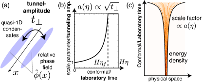
Figure 1: (Color online) Quantum simulator. (a) Sketch of the quantum simulator consisting of a pair of tunnel-coupled 1D bosonic condensates. The tunnel amplitude $t_{\perp}$ is modulated time-dependently. It can be related to the scale parameter $a$ (b) describing the (exponential) expansion of a 1+1 dimensional ’Universe’. The laboratory time (condensate coordinate $x$) is identified with the conformal time $\eta$ (co-moving coordinate) (see main text). The relative phase field between the condensates $\hat{\phi}$ represents the scalar quantum field to be simulated. (c) Semiclassical evaluation of the physical energy density of the simulated quantum field (here displayed in physical coordinates $x_{{\rm ph}}=ax$). One can observe the structure formation out of zero-point quantum fluctuations during the expansion (see main text).

Here, it is argued that a pair of tunnel-coupled, quasi-1D, bosonic condensates (as realized in Schumm et al. (2005) and related experiments) can be employed for simulating an interacting, scalar quantum field on top of an expanding 1+1 dimensional space-time (Fig. 1a,c). This scalar field is represented by the relative phase field between the condensates. As argued in Gritsev et al. (2007); Neuenhahn et al. (2012), at low energies, its dynamics is described by the quantum sine-Gordon model. It turns out that in this setup, one can simulate the expansion of the 1D toy-Universe simply by varying the tunnel-amplitude according to a suitable protocol (Fig. 1b). In the experiments (e.g., Schumm et al. (2005)) the tunnel-amplitude itself can be largely tuned and the field dynamics can be directly visualized by means of matter-wave interferometry. The ’quantumness’ of the relative phase-field dynamics depends on the interaction strength within each condensate (which is easily tunable, e.g., by adapting the 1D condensate density). As far as we are dealing with non-linear dynamics, we consider the weakly interacting, ’semiclassical’ limit (e.g., Polkovnikov (2010); Neuenhahn et al. (2012); Chen et al. (1986)) and employ the truncated Wigner approximation (TWA) (e.g., Polkovnikov (2010)). In contrast, the proposed quantum simulator would allow to explore also the deep quantum regime - in fact, this is its main purpose.

In the following, we start with deriving an effective Hamiltonian description of an interacting quantum field on an expanding 1+1 dimensional space time. In a second step, we introduce the experimental ’quantum simulator’ - the tunnel-coupled condensates - and eventually discuss two of the possible effects, which could be explored.

The first effect is the well known ’freezing’ of quantum fluctuations and the related ’cosmological particle production’ during an accelerating expansion. This purely linear, though most fundamental effect is made responsible for the structure formation in the very early universe Mukhanov (2005). In the present experiments, one can only perform single measurements of the relative phase field per run. Fortunately, this mode freezing also manifests itself in the spatial fluctuation spectrum of the field and thus, in principle, is detectable with single measurements per run. Although, strictly speaking, there is no need for a quantum simulation of the exactly solvable linear dynamics, observing the freeze-out of quantum fluctuations in the experiment would nevertheless be exciting (see for instance Schützhold et al. (2007); Fischer and Schützhold (2004)) and constitute an important check on the setup.

The second feature is the generation of localized, macroscopic structures during the expansion out of quantum fluctuations. This pattern formation involves the full non-linearity of the underlying sine-Gordon field theory and was also observed in the static case Neuenhahn et al. (2012). In contrast to Neuenhahn et al. (2012), for an exponentially fast expansion this happens only for small enough expansion rates. At large expansion times, these patterns seem to turn into standing sine-Gordon breathers simply drifting apart from each other. We argue how to detect signatures of this ’Hubble’ drift experimentally. In cosmology, e.g., dealing with the preheating following inflation, excitations like this (e.g., in the scalar inflaton field) are sometimes denoted as ’oscillons’ (e.g., Amin et al. (2010); Amin and Shirokoff (2010); Gleiser and Sicilia (2009); Gleiser and Howell (2003); Hertzberg (2010); Amin et al. (2012)). A full experimental quantum simulation would allow investigating the formation and persistence of these excitations on an expanding background, even in regimes where quantum effects become very important for the dynamics.

Quantum field on curved space-time. - The space-time action of a classical, scalar field theory in 1+1 dimensions is given by Mukhanov (2005) ($c=1$, $\hbar=1$)

$$\mathcal{S} = \frac{1}{2}\int dx^{2}\sqrt{\left|{\rm det}g_{\mu\nu}\right|}\left[(\partial_{\mu}\chi)g^{\mu\nu}(\partial_{\nu}\chi)-2V(\chi)\right],$$ (1)

where $g_{\mu\nu}$ denotes the metric (with $g_{\mu\nu}g^{\nu\gamma}=\delta_{\mu}^{\gamma}$), $\partial_{\mu}\chi=\partial\chi/\partial x^{\mu}$ and $V(\chi)$ is an arbitrary potential. We are interested in an homogeneous, spatially expanding space-time described by the Friedmann-Robertson-Walker metric (FRW) (see for instance Mukhanov (2005), $ds^{2}=g_{\mu\nu}dx^{\mu}dx^{\nu}$)

$$ds^{2} = d\tau^{2}-a^{2}(\tau)dx^{2}.$$ (2)

Here, $x$ denotes co-moving coordinates which are related to physical coordinates $x_{{\rm ph}}$ via the scale parameter $a(\tau)$ as $x_{{\rm ph}}=ax$. The time $\tau$ denotes the cosmological time, i.e., the proper time of a co-moving observer. In reality, the dynamics of $a$ is determined by Einstein’s equations. Here, we treat $a(\tau)$ as a given function of time, which will be specified below.

In 1+1 dimensions, the Lagrangian corresponding to the action Eq. (1) takes an intriguingly simple form using the so-called conformal time $\eta$ with $d\eta=d\tau/a$:

$$L = \frac{1}{2}\int dx\,\left[\left(\partial_{\eta}\chi\right)^{2}-\left(\partial_{x}\chi\right)^{2}-2a^{2}(\eta)V(\chi)\right].$$ (3)

Note that light geodesics ($ds^{2}=0$) are described by $x(\eta)=\pm\eta+{\rm const}$. The quantization of the field theory follows the standard prescription (e.g., Mukhanov (2005)). First, from Eq. (3), we construct the canonically conjugated field $\Pi_{\chi}(x,\eta)\equiv\frac{\delta\mathcal{\mathcal{L}}}{\delta\partial_{\eta}\chi}=\partial_{\eta}\chi$. In a second step, we promote the fields to operators demanding that $[\hat{\chi}(x,\eta),\hat{\Pi}_{\chi}(x^{\prime},\eta)]=i\delta(x-x^{\prime})$. Eventually, we can switch to the Hamiltonian formulation introducing the time-dependent Hamiltonian

$$\hat{H}(\eta) = \frac{1}{2}\int dx\,\left[\hat{\Pi}_{\chi}^{2}+\left(\partial_{x}\hat{\chi}\right)^{2}+2a^{2}(\eta)V(\hat{\chi})\right].$$ (4)

Note that all effects of the expanding space-time are now encoded in the time-dependence of $\hat{H}(\eta)$ (cf. Schützhold (2005); Schützhold and Unruh (2012); Amin (2010)).

Tunnel coupled condensates as quantum simulator. - Here, we propose a quantum simulation of the field $\hat{\chi}(x,\eta)$ for the special case of a sine-Gordon potential $V=-m_{0}^{2}\beta^{-2}\cos(\beta\hat{\chi})$. This potential has several interesting properties: The corresponding field theory is interacting and integrable. Second, the sine-Gordon potential appears in the so-called ’natural inflation’ scenario Linde (2007). Third, the sine-Gordon potential supports the formation of ’quasibreathers’ Neuenhahn et al. (2012) (in the cosmology literature denoted as ’oscillons’, e.g., Gleiser and Sicilia (2009); Farhi et al. (2008); Amin et al. (2012); Gleiser and Howell (2003) and references therein).

The quantum simulator (Fig.  1a) consists of two tunnel-coupled quasi-1D condensates of cold, bosonic atoms (e.g., Schumm et al. (2005)) with a time-dependent tunnel amplitude $t_{\perp}$. The laboratory time is identified with the conformal time $\eta$. At low energies, the dynamics of the relative phase field $\beta\hat{\phi}(x,t)/\sqrt{2}=(\hat{\phi}_{1}-\hat{\phi}_{2})/\sqrt{2}$ can be described by the quantum sine-Gordon model Gritsev et al. (2007) (the sound velocity $v_{s}=1$)

$$\hat{H}_{{\rm SG}} = \frac{1}{2}\int_{0}^{L}dx\,\left[\hat{\Pi}^{2}+\left(\partial_{x}\hat{\phi}\right)^{2}-\frac{2m^{2}(\eta)}{\beta^{2}}\cos\beta\hat{\phi}\right].$$ (5)

The relative phase field and the relative density variations $\sqrt{2}\beta^{-1}\hat{\Pi}\equiv\frac{\hat{\pi}_{1}-\hat{\pi}_{2}}{\sqrt{2}}$ form a canonical pair. The tunnel amplitude enters the mass term $m^{2}(\eta)=2\beta^{2}\rho_{0}t_{\perp}(\eta)$, where $\rho_{0}$ is the mean density per condensate. The Luttinger liquid description should be reliable as long as the typical lengthscale of Eq. (5), set by $\sqrt{\hbar v_{s}}/m$, is much larger than the healing length of the condensates $\xi_{h}$ Neuenhahn et al. (2012); Gritsev et al. (2007). This can always achieved by choosing a sufficiently small tunnel amplitude $t_{\perp}(\eta)$. The parameter $\beta$ is related to the Luttinger parameter $K$ as $\beta=\sqrt{2\pi/K}$. For weak interactions $\beta\ll 1$. This is the limit we are considering here. It can be shown that $\beta$ plays the role of Plank’s constant Polkovnikov (2010) and $\beta\ll 1$ corresponds to the semiclassical limit of the quantum sine-Gordon model (see also, e.g., Johnson et al. (1986)). The analysis here (as far as we are dealing with non-linear dynamics) is based on the semiclassical TWA. However, in the experiment one can go deep into the quantum regime corresponding to larger $\beta$ (a rather broad range of values up to $K\sim 50$ is realizable, e.g. Krüger et al. (2010)). The following identifications connect the quantum simulator and the quantum field theory on an expanding background. Identifying the fields $\hat{\chi}\leftrightarrow\hat{\phi}$ and $m^{2}(\eta)=m_{0}^{2}a^{2}(\eta)$ [and thus $a(\eta)\leftrightarrow\sqrt{t_{\perp}(\eta)/t_{\perp}(0)}]$, the dynamics of the relative phase field simulates $\hat{\chi}$ in conformal time and co-moving coordinates. In the remainder, we will always argue in terms of the field $\hat{\phi}$, i.e., we analyze Eq. (5).

Scale parameter and initial state. - We consider an exponential expansion $a(\tau)=e^{H\tau}$ with the ’Hubble constant’ $H=\dot{a}(\tau)/a(\tau)$. Choosing $a(0)=1$, the conformal time is given by $\eta=H^{-1}\left[1-e^{-H\tau}\right]$ and correspondingly $a(\eta)=[1-H\eta]^{-1}$ (see Fig. 1b) with $\eta\in[0,\eta_{f}]$ and $\eta_{f}<1/H$. At $\eta_{f}$, the expansion ends and $a(\eta>\eta_{f})=a_{f}$. The dimensionless parameter $H/m_{0}$ compares the expansion time-scale and the typical internal time scale (at short times) of the system and plays a crucial role throughout the following.

At $\eta=0$, we start in the ground state of massive phonons with a small mass $m_{0}$. In particular, $m_{0}$ is chosen much smaller than the UV cutoff $1\sim 1/\xi_{h}$ (all TWA simulations are performed on a lattice with lattice constant set to one, while keeping $m_{0}a(\eta)\ll 1$ throughout the whole simulation). For finite system size and $\beta\ll 1$, the center-of-mass mode (COM mode) $\hat{\Phi}(\eta)\equiv\frac{1}{L}\int_{0}^{L}dx\,\hat{\phi}(x,\eta)$ needs some special attention. For $L/\xi_{h}\gg 1$, we can treat the COM mode classically such that $\hat{\phi}(x,\eta)\simeq\Phi(\eta)+\delta\hat{\phi}(x,\eta)$. Before, the expansion starts, the COM mode is tuned to some value $\Phi(0)\simeq\Phi_{0}$ with $\beta\Phi_{0}\in[0,\pi]$ ($\Phi^{\prime}(0)/m_{0}\simeq 0)$. As argued in Neuenhahn et al. (2012), such an initial state can be achieved by slowly splitting a single condensate followed by applying a potential gradient between the condensates to tune $\Phi_{0}$.

Freezing out of quantum fluctuations. -

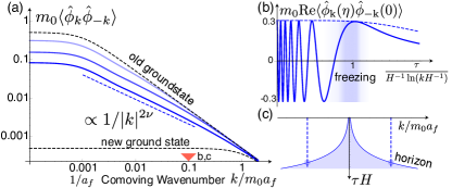
Figure 2: (Color online) Mode ’freezing’. (a) Plot of the spectrum at $a=19.6,166.8,1000$ (blue lines, top to bottom). Here, $H/m_{0}=2.6$ and $m_{0}=0.05$. One observes the spectral tilt (dashed, blue line) resulting from the freezing out of modes. Dashed lines show the corresponding ground state spectra for $a=1$ and $a=a_{f}$. (b) ’Freezing out’ of modes (here $k/a_{f}m_{0}=0.1$). While the suppression of the 1D field fluctuations at later times is non-universal (e.g., it depends on the spatial dimension), the mechanism of the expansion-induced mode freezing is the same as in higher dimensions. (c) Sketch of the horizon crossing

One of the fascinating results of modern cosmology is that the structure formation in the very early Universe seems to have been seeded by quantum fluctuations Mukhanov (2005). This result is truly amazing, as on cosmological scales zero-point fluctuations are tiny. However, it seems that an exponential expansion of the very early Universe (inflationary stage) led to a ’freezing’ of quantum fluctuations and stretched them to cosmological scales. One can reformulate this basic mechanism in a condensed matter language (e.g., Schützhold (2005)). In this terminology, the inflationary expansion corresponds to a rapid, non-adiabatic ’quench’ (see, e.g., Polkovnikov and Gritsev (2008)) producing a large number of excitations (’cosmological particle creation’, cf. Schützhold et al. (2007)).

A very similar effect should be observable in the considered 1+1 dimensional toy-Universe. For this purpose, we consider the case $\Phi_{0}=0$. For small enough $\beta$ and finite system size, one can safely expand the cosine-potential to lowest order $m^{2}(\eta)\beta^{-2}(1-\cos\beta\hat{\phi})\approx\frac{m^{2}(\eta)}{2}\hat{\phi}^{2}$ yielding a theory of massive phonons (cf. Iucci and Cazalilla (2010); De Grandi et al. (2010, 2008); Polkovnikov and Gritsev (2008); Visser and Weinfurtner (2005)) on an expanding 1+1 FRW space-time. According to Eq. (4), the dynamics of the modes $\hat{\phi}_{k}$ [$\hat{\phi}(x,\eta)\equiv\hat{\Phi}+\frac{1}{\sqrt{L}}\sum_{k\neq 0}e^{ikx}\hat{\phi}_{k}(\eta)$] follows as

$$\hat{\phi}_{k}^{\prime\prime}(\eta)+\left[k^{2}+m_{0}^{2}a^{2}(\eta)\right]\hat{\phi}_{k}(\eta) \approx 0.$$ (6)

The general solution of Eq. (6) is given in the Supplement. For $|k|/aH\gg|\nu^{2}-\frac{1}{4}|$ (where $\nu=\frac{1}{2}\sqrt{1-4m_{0}^{2}/H^{2}}$), the modes evolve freely. However, for $|k|/a(\eta)H\sim|\nu^{2}-\frac{1}{4}|$ (cf. Fig. 2b,c), the modes ’freeze’. Most importantly, this ’freezing’ also manifests in the spectrum $\langle\hat{\phi}_{k}(\eta)\hat{\phi}_{-k}(\eta)\rangle$ (cf. Fischer and Schützhold (2004); Schützhold (2005); Mukhanov (2005)). This, in principle allows to observe this effect with a single measurement of the relative phase field $\hat{\phi}(x,\eta)$ per run. For the considered protocol (restricting to $\eta<\eta_{f}$), we obtain for all modes with $|k|\gg H|\nu^{2}-\frac{1}{4}|,m_{0}$ (starting inside the “horizon”) and $|k|/a(\eta)\ll H$ (see Fig. 2a)

$$\langle\hat{\phi}_{k}(\eta)\hat{\phi}_{-k}(\eta)\rangle \propto \frac{1}{a^{1-2\nu}}\frac{H^{2\nu-1}}{|k|^{2\nu}}.$$ (7)

Modes with $|k|/a(\eta)\gg H|\nu^{2}-\frac{1}{4}|$ remain close to the initial ground state of massive phonons with $m_{0}$ yielding $\langle\hat{\phi}_{k}(\eta)\hat{\phi}_{-k}(\eta)\rangle\simeq 1/2|k|$. Here, we consider a fast expansion with $H/m_{0}>2$. In the limit $H/m_{0}\rightarrow\infty$, $\nu$ approaches $1/2$ corresponding to a ’sudden quench’, which leaves the spectrum unchanged. In a possible experiment, one could detect the different power-laws by probing the longitudinal (relative) phase coherence Gritsev et al. (2006) of the condensates on different length-scales (very similar to Gring et al. ). It can be easily checked that the finite $a^{\prime}(0)$ does not influence the ’particle production’ (indicated by the deviations from the instantaneous ground state spectrum [see Eq. (7)]), which happens happens during the evolution.

Formation of breathers out of quantum fluctuations. -

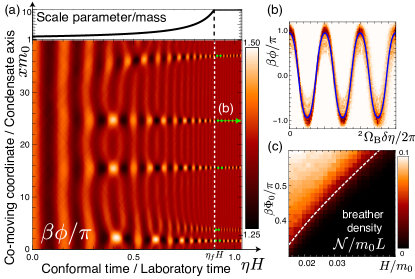
Figure 3: (Color online) Emergence of breathers. (a) Plot of a single TWA run in co-moving coordinates and conformal time ($\beta=0.1$, $\beta\Phi_{0}/\pi=0.65$, $H/m_{0}=0.02$). One observes the damped Josephson oscillations of the COM mode and the emergence of breather-like excitations out of parametrically amplified phonons. As the COM mode is damped away due to the expansion, standing sine-Gordon breathers are released. These can be tracked numerically (green dots). (b) Time-evolution of these breathers tracked at $\delta\eta=0$ denoting the time of tracking ($\eta\geq\eta_{f}$) as a function of $\Omega_{{\rm B}}\delta\eta$ ($\Omega_{{\rm B}}$ is the numerically obtained breather frequency). The spatial center of the breathers is shown. Color code: Distribution function; Blue, solid line shows the temporal evolution of a standing breather (corresponding to the mean breather frequency). (c) Density of created breathers ($\mathcal{N}$ is the number of tracked breathers) obtained by tracking breathers at $a_{f}=10$. Here, $L=1000$, $m_{0}=0.075$ and $\beta=0.1$. The white, dashed line indicates where $\beta{\rm max}_{\eta}\sqrt{\langle\delta\hat{\phi}^{2}\rangle}=0.2$ (see main text).

While the freezing out of quantum fluctuations is a purely linear effect, we now discuss a feature, which heavily relies on interactions. From now on, we consider a slow expansion $H/m_{0}\ll 1$ and finite $0<\Phi_{0}\sim\pi/\beta$ (see Fig. 3a). At short times $\eta>0$, the global relative phase $\Phi(\eta)$ performs Josephson oscillations (see, e.g., Neuenhahn et al. (2012)). However, it is well known that these are parametrically unstable against small, spatial fluctuations (e.g. Bouchoule (2005); Neuenhahn et al. (2012); Greene et al. (1999)). Linearizing around $\Phi$, one finds $\hat{\phi}_{k}^{\prime\prime}+[k^{2}+m_{0}^{2}a^{2}(\eta)\cos\beta\Phi]\hat{\phi}_{k}\simeq 0$. In the static case Neuenhahn et al. (2012), this parametric drive leads to $\hat{\phi}_{k}(\eta)\sim e^{\Gamma(k,\Phi_{0})\eta}$ with $\Gamma\simeq\frac{|k|}{2}\sqrt{\sin^{2}(\beta\Phi_{0}/2)-k^{2}/m^{2}}$ Greene et al. (1999)(displayed for $\beta\Phi_{0}\lesssim 1$). In turn the fluctuations $\langle\delta\hat{\phi}^{2}\rangle$ grow and at some point the linearization breaks down. In the semiclassical limit $\beta\ll 1$, it was demonstrated Neuenhahn et al. (2012) that the non-linearity of the sine-Gordon equations leads to the formation of localized patterns in the field $\hat{\phi}(x,\eta)$. These patterns were identified with ’quasibreather’-solutions of the classical sine-Gordon equation Neuenhahn et al. (2012), which in contrast to usual breathers have a finite lifetime. The ’quasibreather’-solutions could also explain the formation of these excitations out of phononic quantum fluctuations.

Here, for a slow, exponential expansion (in proper time $\tau$), one observes the formation of similar excitations only for $m_{0}/H$ exceeding a certain, almost sharp threshold (Fig. 3c, cf. also Amin et al. (2012)), which depends on $\beta$ and $\Phi_{0}$. To see this, first note that as long as the linearization of the sine-Gordon equation applies, all field fluctuations are suppressed as $\hat{\phi}_{k}\sim 1/\sqrt{a}$ (including the COM mode). Furthermore, in the course of time, resonant modes can get shifted out of resonance as a consequence of the expansion. For a slow expansion, replacing $k\rightarrow k/a$ and $\Phi_{0}\rightarrow\Phi_{0}/\sqrt{a}$ (cf. Greene et al. (1999); Amin et al. (2012)), one finds that $\langle\hat{\phi}_{k}(\eta)\hat{\phi}_{-k}(\eta)\rangle\propto a^{-1}\exp\left[2\int_{0}^{\eta}d\eta^{\prime}\,a\Gamma(\frac{k}{a},\frac{\Phi_{0}}{\sqrt{a}})\right],$which is valid, as long as ${\rm Im\Gamma=0}.$ The non-linearity and thus the formation of localized patterns kicks in only if the fluctuations $\beta\sqrt{\langle\delta\hat{\phi}^{2}(\eta)\rangle}\simeq[\frac{\beta^{2}}{a(\eta)}\int_{2\pi/L}^{k_{c}}\frac{dk}{2\pi}\frac{\exp[2\int_{0}^{\eta}d\eta^{\prime}\,a{\rm Re}\Gamma(\frac{k}{a},\frac{\Phi_{0}}{\sqrt{a}})]}{\sqrt{k^{2}+m_{0}^{2}}}]^{1/2}$ exceed a certain value for some $\eta$ (see Fig.  3c and Material (2012)). Numerically, we find that this value is of the order $\mathcal{O}(10^{-1})$.

Close to the creation threshold, once created, these breather-like excitations persist at the position, where they were ’born’ out of quantum fluctuations. This is in contrast to the ’quasibreathers’ observed in the static case Neuenhahn et al. (2012) (cf. also Farhi et al. (2008)). In the long-time limit, the homogenous part of the field $\Phi$ is damped away $\propto 1/\sqrt{a}$. We find good numerical evidence that the localized excitations, however, are robust against the expansion and can be well described as standing (classical) sine-Gordon breathers $\phi_{{\rm B}}$ (see Fig. 3b). Their typical distance is set by the maximally amplified wavelength before the non-linearity sets in, ending the parametric amplification. It seems that at late times ($a\gg 1$), the only effect of the ’adiabatic’ expansion ($H/m_{0}\ll 1$) on breathers is a trivial shrinking of the breather period and width (both $\propto 1/m_{0}a(\eta)$) in co-moving coordinates, while their amplitude stays approximately constant. This can be understood realizing that the amplitude of a classical sine-Gordon breather $\beta\phi_{{\rm B}}$ is solely determined by the breather parameter $\varphi\in[0,\pi/2]$ (${\rm max}\beta\phi_{{\rm B}}=(2\pi-4\varphi)$, see e.g., Maki and Takayama (1979)). In the quantum sine-Gordon model, this parameter gets quantized Dashen et al. (1975), i.e., it is promoted to a quantum number. However, it is well known that for a slow change of system parameters (by slow, here, we understand $\Omega_{{\rm B}}^{-2}\partial\Omega_{{\rm B}}/\partial\eta\ll 1$, where $\Omega_{{\rm B}}=m_{0}a(\eta)\sin\varphi$ is the instantaneous breather frequency), quantum numbers (and thus the breather amplitude) are approximatively preserved (cf. L.D.Landau and E.M.Lifschitz (2004)).

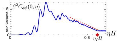
Figure 4: (Color online) Plot of the correlation function $C_{\phi\phi}(0,\eta)$. Clearly, one observes the exponentially growing fluctuations (parametric resonance). At some point the non-linearity of the sine-Gordon model leads to the formation of breather-like structures (around the main peak, cf. Fig. 3a). While the COM mode is damped by the expansion, these structures turn into standing sine-Gordon breathers with a constant amplitude (cf. Fig. 3b), which, in physical coordinates simple drift away from each other. This ’Hubble expansion’ is mirrored by the linear decay of the correlation function as $\propto(1-\eta H)$ at late times. Once the expansion stops at $\eta_{f}$, the correlation function becomes almost constant. Here: $\beta=0.1$, $H/m_{0}=0.02$, $m_{0}=0.05$, $L=800$ and $\beta\Phi_{0}=0.7\pi$.

While for large $a\gg 1$ the number and amplitude of breathers remain constant (per experimental run), they simply move apart from each other in physical coordinates. This ’Hubble expansion’, e.g., can be observed in the (experimentally accessible) equal time correlation $C_{\phi\phi}(x,\eta)=\langle\hat{\phi}(x,\eta)\hat{\phi}(0,\eta)\rangle-\langle\hat{\phi}(0,\eta)\rangle^{2}$ (Fig. 4). Under the assumption that at late times, the field $\hat{\phi}$ can be described as a set of independent (standing) sine-Gordon breathers with fixed amplitudes, one obtains that

$$C_{\phi\phi}(0,\eta) \propto 1-\eta H.$$ (8)

The linear suppression of $C_{\phi\phi}$ is a direct consequence of the decreasing breather density in physical coordinates. From a condensed matter point of view the observation that a suitable protocol for the tunnel-amplitude prepares a state consisting of independent, standing sine-Gordon breathers is interesting by itself. While the analysis here is based on semiclassical considerations (numerically on the TWA) reliable for $\beta\ll 1$, the proposed quantum simulator could for instance test the stability of classical sine-Gordon breathers against quantum fluctuations for larger $\beta\sim 1$ (cf. Dashen et al. (1974)). Furthermore, a quantum simulation could give insight in the excitation of ’oscillonic’ patterns (as discussed in the cosmology community, e.g., Gleiser and Howell (2003); Farhi et al. (2008); Hertzberg (2010); Amin et al. (2012)) in a scalar quantum field (such as the inflaton field or even the Higgs field) during a spatial expansion.

Conclusions. - We demonstrate that tuning the tunnel-amplitude between a pair of tunnel-coupled 1D condensates, the relative phase field can simulate an interacting quantum field on an expanding 1+1 space time. The proposed ’quantum simulator’ should be realizable with present cold atom setups. As examples of the quantum many-body dynamics, which could be investigated, we discussed the freezing out of phonon modes and the creation of sine-Gordon breathers out of quantum fluctuations during an exponential FRW-expansion. While the discussion here is restricted to the semiclassical limit of the underlying quantum sine-Gordon model, the ’quantum simulator’ is meant to explore the deep quantum regime.

Acknowledgements. – We thank R. Schützhold for fruitful discussions related to this work. Financial support by the Emmy-Noether program is gratefully acknowledged.

Supplemental material. – Here, we discuss the dynamics of massive phonons on the expanding 1+1 dimensional space-time in conformal time following Eq. (6). The classical solution is given by

$$\phi_{k}(\eta) = \frac{C_{k}^{+}}{\sqrt{a}}J_{\nu}(\frac{|k|}{aH})+\frac{C_{k}^{-}}{\sqrt{a}}J_{-\nu}(\frac{|k|}{aH}),$$ (9)

where $\nu=\frac{1}{2}\sqrt{1-4m_{0}^{2}/H^{2}}$ and $J_{\nu}$ denotes the Bessel function of the first kind. In the following, we restrict to $H/m_{0}>2$. The quantum mechanical solution follows from Eq. (9) promoting the coefficients $C_{k}^{\pm}$ to operators $\hat{C}_{k}^{\pm}$ and by matching the initial conditions at $\eta=0$ ($a=1$), i.e., $\hat{\phi}_{k}(0)=\frac{1}{\sqrt{2\omega_{k}(m_{0})}}(\hat{b}_{k}+\hat{b}_{-k}^{\dagger})$ and $\hat{\phi}_{k}^{\prime}(0)=-i\sqrt{\frac{\omega_{k}(m_{0})}{2}}(\hat{b}_{k}-\hat{b}_{-k}^{\dagger})$. Here, $\omega_{k}(m_{0})=\sqrt{k^{2}+m_{0}^{2}}$ is the dispersion of massive phonons and $\hat{b}_{k}|0\rangle=0$ ($|0\rangle$ denotes the ground state of massive phonon modes with $k\neq 0$ and mass $m_{0}$, in which the system is initialized). As $J_{\nu}(x>0)\in\mathbb{R}$ for ${\rm Im\nu=0}$, we obtain

$$\hat{C}_{k}^{+} = \underbrace{\left[\frac{j_{-\nu}/\sqrt{2\omega_{k}}+iJ_{-\nu}\sqrt{\omega_{k}/2}}{j_{-\nu}J_{\nu}-j_{\nu}J_{-\nu}}\right]}_{\alpha_{k}}\hat{b}_{k}+\alpha_{k}^{\ast}\hat{b}_{-k}^{\dagger},$$ (10)

$$\hat{C}_{k}^{-} = \underbrace{\left[\frac{1}{\sqrt{2\omega_{k}}J_{-\nu}}-\alpha_{k}\frac{J_{\nu}}{J_{-\nu}}\right]}_{\beta_{k}}\hat{b}_{k}+\beta_{k}^{\ast}\hat{b}_{-k}^{\dagger},$$ (11)

where we introduced the abbreviations $j_{\pm\nu}=\left.\partial_{\eta}(a^{-1/2}J_{\pm\nu}\left[\frac{|k|}{aH}\right])\right|_{\eta=0}$ and $J_{\pm\nu}=J_{\pm\nu}\left[\frac{|k|}{H}\right]$. The fluctuation spectrum yields

$$\langle 0|\hat{\phi}_{k}^{\dagger}(\eta)\hat{\phi}_{k}(\eta)|0\rangle = \frac{|\alpha_{k}J_{\nu}\left(\frac{|k|}{aH}\right)+\beta_{k}J_{-\nu}\left(\frac{|k|}{aH}\right)|^{2}}{a(\eta)}.$$ (12)

We are interested in modes starting within the horizon, i.e., with $|k|\gg H|\nu^{2}-\frac{1}{4}|,m_{0}$. Making use of the limits

$$\lim_{x/|\nu^{2}-\frac{1}{4}|\rightarrow\infty}J_{\nu}(|x|) = -\sqrt{\frac{2}{\pi x}}\sin(\frac{\pi\nu}{2}-x-\frac{\pi}{4}),$$

$$\lim_{x\rightarrow 0}J_{\nu}(|x|) = \frac{|x|^{\nu}}{2^{\nu}\Gamma(\nu+1)},$$ (13)

one obtains for large times $\eta$, such that $|k|/a(\eta)H\ll 1$ (and finite $\nu$):

$$\langle 0|\hat{\phi}_{k}^{\dagger}\hat{\phi}_{k}|0\rangle \simeq \frac{1}{H^{1-2\nu}a(\eta)^{1-2\nu}}\frac{1}{|k|^{2\nu}}.$$ (14)

References

- Greiner et al. (2002) M. Greiner, O. Mandel, T. W. Hansch, and I. Bloch, Nature 419, 51 (2002).
- Kinoshita et al. (2006) T. Kinoshita, T. Wenger, and D. S. Weiss, Nature 440, 900 (2006).
- Hofferberth et al. (2007) S. Hofferberth, I. Lesanovsky, B. Fischer, T. Schumm, and J. Schmiedmayer, Nature 449, 324 (2007).
- Lanyon et al. (2011) B. P. Lanyon, C. Hempel, D. Nigg, M. Müller, R. Gerritsma, F. Zöhringer, P. Schindler, J. T. Barreiro, M. Rambach, G. Kirchmair, M. Hennrich, P. Zoller, R. Blatt, and C. F. Roos, Science 334, 57 (2011), http://www.sciencemag.org/content/334/6052/57.full.pdf .
- Bloch et al. (2008) I. Bloch, J. Dalibard, and W. Zwerger, Reviews of Modern Physics 80, 885 (2008).
- Jordan et al. (2012) S. P. Jordan, K. S. M. Lee, and J. Preskill, Science 336, 1130 (2012), http://www.sciencemag.org/content/336/6085/1130.full.pdf .
- Buluta and Nori (2009) I. Buluta and F. Nori, Science 326, 108 (2009), http://www.sciencemag.org/content/326/5949/108.full.pdf .
- Garay et al. (2000) L. J. Garay, J. R. Anglin, J. I. Cirac, and P. Zoller, Phys Rev Lett 85, 4643 (2000).
- Fischer and Schützhold (2004) U. R. Fischer and R. Schützhold, Phys. Rev. A 70, 063615 (2004).
- Schützhold et al. (2007) R. Schützhold, M. Uhlmann, L. Petersen, H. Schmitz, A. Friedenauer, and T. Schätz, Phys. Rev. Lett. 99, 201301 (2007).
- Jain et al. (2007) P. Jain, S. Weinfurtner, M. Visser, and C. W. Gardiner, Phys. Rev. A 76, 033616 (2007).
- Prain et al. (2010) A. Prain, S. Fagnocchi, and S. Liberati, Phys. Rev. D 82, 105018 (2010).
- Unruh (1981) W. Unruh, Phys. Rev. Lett. 46 (1981).
- Visser and Weinfurtner (2005) M. Visser and S. Weinfurtner, Phys. Rev. D 72, 044020 (2005).
- Barceló et al. (2011) C. Barceló, S. Liberati, and M. Visser, Living Rev. Relativity 14 (2011).
- Schützhold (2005) R. Schützhold, Phys. Rev. Lett. 95, 135703 (2005).
- Schumm et al. (2005) T. Schumm, S. Hofferberth, L. M. Andersson, S. Wildermuth, S. Groth, I. Bar-Joseph, J. Schmiedmayer, and P. Krüger, Nature Physics 1, 57 (2005).
- Gritsev et al. (2007) V. Gritsev, A. Polkovnikov, and E. Demler, Phys. Rev. B 75, 174511 (2007).
- Neuenhahn et al. (2012) C. Neuenhahn, A. Polkovnikov, and F. Marquardt, arXiv:1112.5982v1 (2012).
- Polkovnikov (2010) A. Polkovnikov, Annals of Phys. 325 (2010).
- Chen et al. (1986) N.-N. Chen, M. D. Johnson, and M. Fowler, Phys. Rev. Lett. 56, 904 (1986).
- Mukhanov (2005) V. Mukhanov, Cambridge University Press (2005).
- Amin et al. (2010) M. A. Amin, R. Easther, and H. Finkel, Journal of Cosmology and Astroparticle Physics 12 (2010).
- Amin and Shirokoff (2010) M. A. Amin and D. Shirokoff, Phys. Rev. D 81, 085045 (2010).
- Gleiser and Sicilia (2009) M. Gleiser and D. Sicilia, Phys. Rev. D 80, 125037 (2009).
- Gleiser and Howell (2003) M. Gleiser and R. C. Howell, Phys. Rev. E 68, 065203 (2003).
- Hertzberg (2010) M. P. Hertzberg, Phys. Rev. D 82, 045022 (2010).
- Amin et al. (2012) M. A. Amin, R. Easther, H. Finkel, R. Flauger, and M. P. Hertzberg, Phys. Rev. Lett. 108, 241302 (2012).
- Schützhold and Unruh (2012) R. Schützhold and W. G. Unruh, arXiv:1203.1173v1 (2012).
- Amin (2010) M. A. Amin, arXiv:1006.3075v2 (2010).
- Linde (2007) A. Linde, in Inflationary Cosmology, Lecture Notes in Physics, Vol. 738, edited by M. Lemoine, J. Martin, and P. Peter (Springer Berlin / Heidelberg, 2007) pp. 1–54.
- Farhi et al. (2008) E. Farhi, N. Graham, A. H. Guth, N. Iqbal, R. R. Rosales, and N. Stamatopoulos, Phys. Rev. D 77, 085019 (2008).
- Johnson et al. (1986) M. D. Johnson, N.-N. Chen, and M. Fowler, Phys. Rev. B 34, 7851 (1986).
- Krüger et al. (2010) P. Krüger, S. Hofferberth, I. E. Mazets, I. Lesanovsky, and J. Schmiedmayer, Phys. Rev. Lett. 105, 265302 (2010).
- Polkovnikov and Gritsev (2008) A. Polkovnikov and V. Gritsev, Nat Phys 4, 477 (2008).
- Iucci and Cazalilla (2010) A. Iucci and M. A. Cazalilla, New Journal of Physics 12, 055019 (2010).
- De Grandi et al. (2010) C. De Grandi, V. Gritsev, and A. Polkovnikov, Phys. Rev. B 81, 224301 (2010).
- De Grandi et al. (2008) C. De Grandi, R. A. Barankov, and A. Polkovnikov, Phys. Rev. Lett. 101, 230402 (2008).
- Gritsev et al. (2006) V. Gritsev, E. Altman, E. Demler, and A. Polkovnikov, Nat Phys 2, 705 (2006).
- (40) M. Gring, M. Kuhnert, T. Langen, T. Kitagawa, B. Rauer, M. Schreitl, I. Mazets, D. A. Smith, E. Demler, and J. Schmiedmayer, arXiv:1112.0013v1 .
- Bouchoule (2005) I. Bouchoule, Eur. Phys. J. D , 147 (2005).
- Greene et al. (1999) P. B. Greene, L. Kofman, and A. A. Starobinsky, Nuclear Physics B , 423 (1999).
- Material (2012) S. Material, (2012).
- Maki and Takayama (1979) K. Maki and H. Takayama, Phys. Rev. B 20, 5002 (1979).
- Dashen et al. (1975) R. F. Dashen, B. Hasslacher, and A. Neveu, Phys. Rev. D 11, 3424 (1975).
- L.D.Landau and E.M.Lifschitz (2004) L.D.Landau and E.M.Lifschitz, Mechanik (Verlag Harri Deutsch, 2004).
- Dashen et al. (1974) R. F. Dashen, B. Hasslacher, and A. Neveu, Phys. Rev. D 10, 4130 (1974).