Solar Magnetic Field Reversals and the Role of Dynamo Families

Abstract

The variable magnetic field of the solar photosphere exhibits periodic reversals as a result of dynamo activity occurring within the solar interior. We decompose the surface field as observed by both the Wilcox Solar Observatory and the Michelson Doppler Imager into its harmonic constituents, and present the time evolution of the mode coefficients for the past three sunspot cycles. The interplay between the various modes is then interpreted from the perspective of general dynamo theory, where the coupling between the primary and secondary families of modes is found to correlate with large-scale polarity reversals for many examples of cyclic dynamos. Mean-field dynamos based on the solar parameter regime are then used to explore how such couplings may result in the various long-term trends in the surface magnetic field observed to occur in the solar case.

1 Introduction

The Sun is a dynamic star that possesses quasi-regular cycles of magnetic activity having a mean period of about 22 yr. This period varies from cycle to cycle, and over the past several centuries has ranged from 18 to 25 years (Weiss 1990; Beer et al. 1998; Usoskin et al. 2007), as for example illustrated by the unusual but not unprecedented length of the most recently completed sunspot cycle 23. During each sunspot cycle (comprising half of a magnetic cycle), the Sun emerges sunspot groups and active regions onto the photosphere, with such features possessing characteristic latitudes, polarity, and tilt angles. As with the period, the numbers and emergence frequencies of active regions is observed to vary from cycle to cycle.

At activity minima when few active regions are present, the surface magnetic field is characterized by the presence of two polar caps, i.e., largely unipolar patches of magnetic flux dispersed across both polar regions with the northern and southern caps possessing opposite polarities. Reversals of this large-scale dipole represented by the polar-cap flux occur during each sunspot cycle, allowing the subsequent sunspot cycle to begin in the opposite configuration. After two sunspot cycles, and thus after undergoing two polarity reversals, the photospheric field will have returned to its starting configuration so as to complete a full activity cycle.

In response to the photospheric flux associated with various features, such as active regions and their decay products, the coronal magnetic field possesses structures having a broad spectrum of sizes. These structures are both evident in observations of coronal loops, as found in narrow-band extreme ultraviolet or soft X-ray imagery, and reproduced in models of the coronal magnetic field (e.g., Schrijver & DeRosa 2003). In both venues, the coronal magnetic field geometry is seen to contain a rich and complex geometry. Dynamical events originating from the corona, such as eruptive flares and coronal mass ejections, are likely powered by energy released by a reconfiguration of the coronal magnetic field, which in turn is responding to changes and evolution of photospheric fields.

Precise measurements of the time-history of photospheric magnetic field and the ability to determine the projection of this field into its constituent multipole components are helpful in investigating the physical processes thought to be responsible for dynamo activity (Bullard & Gellman 1954; Moffatt 1978). In cool stars similar to the Sun, the dynamo is presumed to be a consequence of the nonlinear interactions between convection, rotation, and large scale flows, leading to the generation and maintenance against Ohmic diffusion of magnetic field of various temporal and spatial scales (Weiss 1987; Cattaneo 1999; Ossendrijver 2003; Brun et al. 2004; Vögler & Schüssler 2007; Charbonneau 2010; Reiners 2012). In particular, the dependence of dynamo activity upon rotation appears to be well established (Noyes et al. 1984; Saar & Brandenburg 1999; Pizzolato et al. 2003; Böhm-Vitense 2007; Reiners et al. 2009). However, many details of the understanding of why many cool-star dynamos excite waves of dynamo activity having a regular period, specifically 22 yr in the case of the Sun, remain unclear.

To investigate this question, it is useful to explore the behavior and evolution of the lowest-degree (i.e., largest-scale) multipoles, their amplitudes and phases, and their correlations with the solar photospheric magnetic field. Many earlier studies (e.g., Levine 1977; Hoeksema 1984; Gokhale et al. 1992; Gokhale & Javaraiah 1992) have illustrated how power in these modes ebb and flow as a function of the activity level. In particular, J. Stenflo and collaborators have performed thorough spectral analyses on the temporal evolution of the various spherical harmonic modes. Stenflo & Vogel (1986), Stenflo & Weisenhorn (1987), and Stenflo & Güdel (1988), and more recently Stenflo (1994) and Knaack & Stenflo (2005), base their analysis on Mt. Wilson and Kitt Peak magnetic data spanning the past few sunspot cycles. As one would expect, they find that most of the power is contained in temporal modes having a period of about 22 yr, and especially in spherical harmonics that are equatorially antisymmetric, such as the axial dipole and octupole. However, they find signatures of the activity cycle are present in all axisymmetric harmonics, as significant power is present at temporal frequencies at or near integer multiples of the fundamental frequency of 1.44 nHz [equivalent to (22 yr)^-1].

In the current study, we focus on the coupling between spherical harmonic modes, and what such coupling may indicate about the operation of the interior dynamo. In particular, reversals of the axial dipole mode may be viewed as a result of continuous interactions between the poloidal and toroidal components of the interior magnetic field, i.e., the so-called dynamo loop. Currently, one type of solar dynamo model that successfully reproduces many observed behaviors is the flux-transport Babcock-Leighton type (e.g., Choudhuri et al. 1995; Dikpati et al. 2004; Jouve & Brun 2007; Yeates et al. 2008). A key ingredient in producing realistic activity cycles using this type of model is found to be the amplitude and profile of the meridional flow (Jouve & Brun 2007; Karak 2010; Nandy et al. 2011; Dikpati 2011), which result in field reversals progressing via the poleward advection across the surface of trailing-polarity flux from emergent bipolar regions. During the rising phase of each sunspot cycle, polar cap flux left over from the previous cycle is canceled, after which new polar caps having the opposite magnetic polarity form (Wang et al. 1989; Benevolenskaya 2004; Dasi-Espuig et al. 2010).

Helioseismic analyses of solar oscillations have provided measurements and inferences of key dynamo components, such as the internal rotation profile and the near-surface meridional circulation (Thompson et al. 2003; Basu & Antia 2010). Complementing precise observations of the solar magnetic cycle properties, these helioseismic inversions represent additional strong constraints on theoretical solar dynamo models. Successful solar dynamo models strive to reproduce as many empirical features of solar magnetic activity as possible, including not only cycle periods, but also parity, phase relation between poloidal and toroidal components, and the phase relation between the dipole and higher-degree harmonic modes.

Interestingly, a recent analysis of geomagnetic records has indicated that the interplay between low-degree harmonic modes during polarity reversals is one way to characterize both reversals of the geomagnetic dynamo (which have a mean period of about 300,000 yr) as well as excursions, where the dipole axis temporarily moves equatorward and thus away from its usual position of being approximately aligned with the rotation axis, followed by a return to its original position without having crossed the equator (see Hulot et al. 2010 for a recent review on Earth’s magnetic field). In particular, these studies have shown that, during periods of geomagnetic reversals, the quadrupolar component of the geomagnetic field is stronger than the dipolar component, while during an excursion (which can be thought of as a failed reversal), the dipole remains dominant (Amit et al. 2010; Leonhardt & Fabian 2007; Leonhardt et al. 2009). One may thus ask: Is a similar behavior observed for the solar magnetic field?

In an attempt to address this question, we have performed a systematic study of the temporal evolution of the solar photospheric field by determining the spherical harmonic coefficients for the photospheric magnetic field throughout the past three sunspot cycles, focusing on low-degree modes and the relative amplitude of dipolar and quadrupolar components. Following the classification of McFadden et al. (1991), we have made the distinction between primary and secondary families of harmonic modes, a classification scheme that takes into account the symmetry and parity of the spherical harmonic functions (see Gubbins & Zhang 1993 for a detailed discussion on symmetry and dynamo).

While we recognize that the solar dynamo operates in a more turbulent parameter regime than the geodynamo, and is more regular in its reversals, the presence of grand minima (such as the Maunder Minimum) in the historical record indicates that the solar dynamo can switch to a more intermittent state on longer-term, secular time scales. In fact in the late stages of the Maunder Minimum, the solar dynamo was apparently asymmetric, with the southern hemisphere possessing more activity than the north (Ribes & Nesme-Ribes 1993) for several decades, a magnetic configuration that may have been achieved by having dipolar and quadrupolar modes of similar amplitude (Tobias 1997; Gallet & Pétrélis 2009). Additionally, recent spectopolarimetric observations of solar-like stars now provide sufficient resolution to characterize the magnetic field geometry in terms of its multipolar decomposition (Petit et al. 2008). Furthermore, the analysis of reduced dynamical systems developed over the last 20 yr describing the geodynamo and solar dynamo have emphasized the importance of the nonlinear coupling between dipolar and quadrupolar components (Knobloch & Landsberg 1996; Weiss & Tobias 2000; Pétrélis et al. 2009).

This article is organized in the following manner. In §2, we describe the data sets and the data analysis methods used to perform the spherical harmonic analysis, followed in §3 with an explanation of the temporal evolution of the various harmonic modes, the magnetic energy spectra, and the decomposition in terms of primary and secondary families. We interpret in §4 our results from a dynamical systems perspective and illustrate some of these concepts using mean-field dynamo models. Concluding remarks are presented in §5.

2 Observations and Data Processing

We analyze time series of synoptic photospheric magnetic field maps of the radial magnetic field $B_{r}$ derived from line-of-sight magnetogram observations taken by both the Wilcox Solar Observatory (WSO; Scherrer et al. 1977) at Stanford University and by the Michelson Doppler Imager (MDI; Scherrer et al. 1995) on board the space-borne Solar and Heliospheric Observatory (SOHO). The WSO data used in this study span the past 36 years, commencing with Carrington Rotation (CR) 1642 (which began on 1976 May 27) and ending with CR 2123 (which ended on 2012 May 25). For MDI, we used data from much of its mission lifetime, starting with CR 1910 (which began on 1996 Jul. 1) through CR 2104 (which ended on 2010 Dec. 24). In both data series, one map per Carrington rotation was used, though maps with significant amounts of missing data were excluded. The measured line-of-sight component of the field is assumed to be the consequence of a purely radial magnetic field when calculating the harmonic coefficients. Additionally, for WSO, the synoptic map data are known to be a factor of about 1.8 too low due to the saturation of the instrument (Svalgaard et al. 1978). Lastly, the MDI data have had corrections applied for the polar fields using the interpolation scheme presented in Sun et al. (2011).

For each map, we perform the harmonic analysis using the Legendre-transform software provided by the “PFSS” package available through SolarSoft. Using this software first entails remapping the latitudinal dimension of the input data from the sine-latitude format provided by the observatories onto a Gauss-Legendre grid (c.f., § 25.4.29 of Abramowitz & Stegun 1972). This regridding enables Gaussian quadrature to be used when evaluating the sums needed to project the magnetic maps onto the spherical harmonic functions. The end result is a time-varying set of complex coefficients $B_{\ell}^{m}(t)$ for a series of modes spanning harmonic degrees $\ell$ = 0, 1, …, $\ell_{\max}$, where the truncation limit $\ell_{\max}$ is equal to 60 for the WSO maps and 192 for MDI maps. The $B_{\ell}^{m}$ coefficients are proportional to the amplitude of each spherical harmonic mode $Y_{\ell}^{m}$ for degree $\ell$ and order $m$ possessed by the time series of synoptic maps, so that

$$B_{r}(\theta,\phi,t)=\sum_{\ell=0}^{\ell_{\max}}\sum_{m=0}^{\ell}B_{\ell}^{m}(t)\,Y_{\ell}^{m}(\theta,\phi),$$ (1)

where $\theta$ is the colatitude, $\phi$ is the latitude, and $t$ is time. We note that because the coefficients $B_{\ell}^{m}$ are complex numbers, this naturally accounts for the rotational symmetry between spherical harmonic modes with orders $m$ and $-m$ (for a given value of $\ell$), with the amplitudes of modes for which $m>0$ appearing in the real part of $B_{\ell}^{m}$, and the amplitudes of the modes where $m<0$ being contained in the imaginary part of $B_{\ell}^{m}$. Consequently, the sum over $m$ in equation (1) starts at $m=0$ instead of at $m=-\ell$. The coefficients $B_{\ell}^{0}$ corresponding to the axisymmetric modes (for which $m=0$) are real for all $\ell$.

We use the convention that, for a particular spherical harmonic degree $\ell$ and order $m$,

$$Y_{\ell}^{m}(\theta,\phi)=C_{\ell}^{m}P_{\ell}^{m}(\cos\theta)\,e^{im\phi},$$ (2)

where the functions $P_{\ell}^{m}(\cos\theta)$ are the associated Legendre polynomials, and where the coefficients $C_{\ell}^{m}$ are defined

$$C_{\ell}^{m}=(-1)^{m}\left[\frac{2\ell+1}{4\pi}\frac{(\ell-m)!}{(\ell+m)!}\right]^{\frac{1}{2}}.$$ (3)

With this normalization, the spherical harmonic functions satisfy the orthogonality relationship

$$\int_{0}^{2\pi}d\phi\int_{0}^{\pi}\sin\theta\,d\theta\,Y_{\ell}^{m*}Y_{\ell^{\prime}}^{m^{\prime}}=\delta_{\ell\ell^{\prime}}\,\delta_{mm^{\prime}}.$$ (4)

When comparing our coefficients with those from other studies, it is important to take the normalization into account. For example, the complex $B_{\ell}^{m}$ coefficients used here are different than (albeit related to) the real-valued $g_{\ell}^{m}$ and $h_{\ell}^{m}$ coefficients provided by the WSO team. This difference is due to their use of spherical harmonics having the Schmidt normalization, a convention that is commonly used by the geomagnetic community as well as by earlier studies in the solar community such as Altschuler & Newkirk (1969). For the WSO data used here, we have verified that the values of $B_{\ell}^{m}$ used in this study are commensurate with the $g_{\ell}^{m}$ and $h_{\ell}^{m}$ coefficients provided by the WSO team.

Because we possess perfect knowledge of $B_{r}$ neither over the entire Sun nor at one instant in time, the monopole coefficient function $B_{0}^{0}(t)$ does not strictly vanish and instead fluctuates around zero. In practice, we find that the magnitude of $B_{0}^{0}(t)$ is small, and thus feel justified in not considering it further. This assumption effectively means that from each magnetic map we are subtracting off any excess net flux, $\oint B_{r}(\theta,\phi)\,\sin\theta\,d\theta\,d\phi$, a practice which leads to the introduction of small errors in the resulting analysis. However, these errors are deemed to be less important than the inaccuracies resulting from the less-than-perfect knowledge of the radial magnetic flux on the Sun, including effects due to evolution and temporal sampling throughout each Carrington rotation and due to the lack of good radial field measurements of the flux in the polar regions of the Sun.

3 Multipolar Expansions and Their Evolution as a Function of Cycle

3.1 Dipole Field (Modes with $\boldsymbol{\ell}=1$)

The solar dipolar magnetic field can be analyzed in terms of its axial and equatorial harmonic components. As has long been known (Hoeksema 1984), the axial dipole component, having a magnitude of $|B_{1}^{0}|$, is observed to be largest during solar minimum when there is a significant amount of magnetic flux located at high heliographic latitudes on the Sun. These two so-called polar caps possess opposite polarity, and match the polarity of the trailing flux within active regions located in the corresponding hemisphere that emerged during the previous sunspot cycle. Long-term observations of surface-flux evolution indicate that a net residual amount of such trailing-polarity flux breaks off from decaying active regions and is released into the surrounding, mixed-polarity quiet-sun network. This flux is observed to continually evolve as flux elements merge, fragment, and move around in response to convective motions (Schrijver et al. 1997), but the long-term effect is that the net residual flux is slowly advected poleward by surface meridional flows. Such poleward advection results in a net influx of trailing-polarity flux into the higher latitudes. At the same time, an equivalent amount of leading-polarity flux from each hemisphere cancels across the equator, as is necessary to balance the trailing-polarity flux advected poleward. Over the course of a sunspot cycle, this process is repeated throughout subsequent sunspot cycles, during which flux from the trailing polarities of active regions eventually cancels out the polar-cap flux left over from previous cycles. Once the leftover flux has fully disappeared, the buildup of a new polar cap having the opposite polarity occurs by the subsequent activity minimum.

In contrast to the axial dipole component, the equatorial dipole components, having magnitudes $|B_{1}^{-1}|$ and $|B_{1}^{1}|$, are largest during maximum activity intervals and weakest during activity minima. Individual active regions on the photosphere each contribute a small dipole moment that, aside from the small axial component arising from the Joy’s Law tilt, is oriented in the equatorial plane. Together the equatorial dipole moments from the collection of active regions add vectorially to form the overall dipole moment. When many active regions are on the disk, it thus follows that the equatorial dipole mode is likely to have a higher amplitude. During periods of quiet activity with few active regions on disk, the equatorial dipole amplitude is minimal.

Because the WSO data span three sunspot activity cycles, a bit of historical perspective on the evolution of the dipole can be gained, as shown in Figure 1. Figure 1(a) shows the amplitude of the axial dipole moment since mid 1976 and its evolution as a function of the activity level, represented in the figure by the sunspot number (SSN). It is also evident that, during the most recent minimum prior to Cycle 24, the magnitude of the axial dipole component is much lower than during any of the three previous minima (i.e., those preceding Cycles 21–23). The connection between the axial dipole component and the flux in the northern hemisphere is illustrated in the time-history of the mean flux density as integrated over the northern hemisphere, shown in Figure 2. We observe a slight lag for the northern hemisphere averaged magnetic flux with respect to the axial dipole coefficient due to the contribution of other axisymmetric modes possessing a different phase.

Figure 1(b) illustrates the magnitude of the equatorial dipole since mid 1976. In step with the relatively lower number of active regions during Cycle 23 when compared with the maxima for Cycles 21 and 22, the equatorial dipole strength is found to be lower during the most recent maximum than during the maxima corresponding to Cycles 21 or 22.

Given the variation in sunspot cycle strengths throughout the past few centuries, we suspect that cycle-to-cycle variations in the magnitudes of the axial and equatorial modes are not unusual. Proxies of the historical large-scale magnetic field, such as cosmic-ray induced variations of isotopic abundances measured from ice-core data (Steinhilber et al. 2012), also show such longer-term variation and thus seem to be consistent with this view. Interestingly, the range over which the variation in the ratio of the energies possessed by the equatorial versus the axial dipole components is about the same for the three sunspot cycles observed by WSO, as shown in Figure 1(c). Longer-term measurements of this ratio unfortunately are not available due to the lack of a sequence of long-term magnetogram maps to which the harmonic decomposition analysis outlined in Section 2 can be applied.

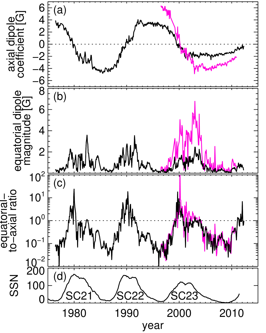
Figure 1: Evolution of the dipole ($\ell=1$) modes, as characterized by the (a) axial dipole coefficient $B_{1}^{0}$, (b) equatorial dipole magnitude $\sqrt{(B_{1}^{-1})^{2}+(B_{1}^{1})^{2}}$, and (c) the ratio of their energies $[(B_{1}^{-1})^{2}+(B_{1}^{1})^{2}]/(B_{1}^{0})^{2}$ for the WSO (black) and MDI polar-corrected (magenta) data sets. Panel (d) shows the monthly smoothed sunspot number (SSN) from Solar Influences Data Center at the Royal Observatory of Belgium. The WSO data have not been corrected for known saturation effects that reduce the reported values by a factor of 1.8 (Svalgaard et al. 1978).

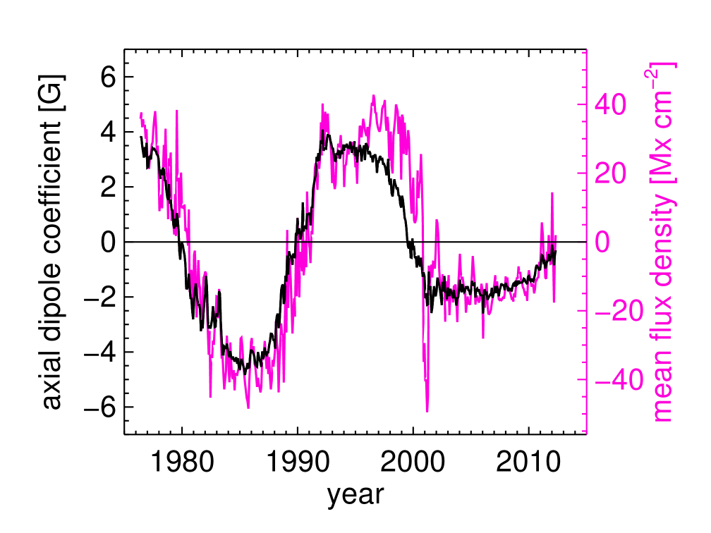
Figure 2: Northern hemispheric mean flux density (magenta) and axial dipole coefficient from WSO (black), illustrating the connection between the axial dipole and the flux in each hemisphere. The downward spike in the mean hemispheric flux density occurring in 2001 is likely related to WSO sensitivity issues occurring during that time period, and may not be real.

3.2 Reversals of the Dipole

The process by which old polar caps are canceled out and replaced with new, opposite-polarity polar caps, as described in the previous section, manifests itself as a change in sign of the axial dipole amplitude throughout the course of a sunspot cycle. Such dipole reversals for the past three sunspot cycles are shown in Figure 3, where the latitude and longitude of the dipole axis are plotted with time. It is found that the dipole axis spends much of its time in the polar regions, and for only about 12–18 months during these cycles is it located equatorward of $\pm$45^∘.

During these reversals, which occur at or near maximal activity intervals, the energy in the dipole never completely disappears. We find that the reduction in the energy $(B_{1}^{0})^{2}$ in the the axial dipole is partially offset by an increase in the energy $(B_{1}^{-1})^{2}+(B_{1}^{1})^{2}$ in the equatorial dipole. This results in a reduction of the total energy $\sum_{m}(B_{1}^{m})^{2}$ in all dipolar modes only by about an order of magnitude from its axial-dipole-dominated value at solar minimum, as shown in Figure 4(a).

Figure 3 indicates that, during a reversal when the axial dipolar component is weak, the axis of the equatorial dipolar component wanders in longitude. This seemingly aimless wandering occurs because the longitude of the dipole axis is primarily determined by an interplay amongst the strongest active regions on the photosphere at the time of observation. As older active regions decay and newer active regions emerge onto the photosphere, the equatorial-dipolar axis responds in kind.

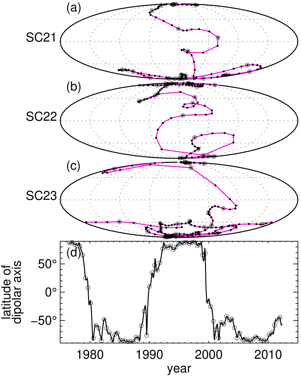
Figure 3: (a)–(c) Mollweide projections of the location of the dipole axis for the past three sunspot cycles (Cycles 21–23), as determined from WSO synoptic charts. The solid circles indicate the longitude and latitude of the dipole axis for each Carrington rotation, with every sixth Carrington rotation also indicated by an open circle. Grid lines (dashed) are placed every 45^∘ in latitude and longitude for reference. The Carrington longitudes of the central meridians of each projection are chosen to best illustrate the reversals, and differ in each of the panels. Panel (d) illustrates the latitude of the dipole axis as a function of time. The open circles in panel (d) correspond to same times as the open circles in panels (a)–(c).

3.3 Quadrupole Field (Modes with $\boldsymbol{\ell}=2$)

The evolution of the energy contained in the quadrupolar ($\ell=2$) modes exhibit much more variation than the dipole, as shown in Figure 4. As with the equatorial dipole components, all of the quadrupolar modes have more power during greater activity intervals than during quieter periods, as illustrated in the evolution of the various quadrupolar modes plotted in Figure 5. Furthermore, when large amounts of activity occur, it is possible for the total energy $\sum_{m}(B_{2}^{m})^{2}$ in all quadrupolar modes to be greater than the energy $\sum_{m}(B_{1}^{m})^{2}$ in the dipolar modes at the photosphere. The ratio between these two groups of modes is shown in Figure 4(c), from which it is evident that during each of the past three sunspot cycles there have been periods of time when the quadrupolar energy exceeded the dipolar energy by as much as a factor of 10. The corona, in turn, reflects the relative strength of a strong quadrupolar configuration of photospheric magnetic fields by creating complex sectors and possibly multiple current sheets that extend into the heliosphere. One example of such complex field geometry is suggested by the potential-field source-surface model of Figure 6, where a quadrupolar configuration having an axis of symmetry lying almost in the equatorial plane is seen to predominate.

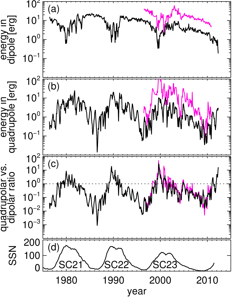
Figure 4: Total energy in (a) dipolar modes $\sum_{m}(B_{1}^{m})^{2}$, (b) quadrupolar modes $\sum_{m}(B_{2}^{m})^{2}$, and (c) their ratio $\sum_{m}(B_{2}^{m})^{2}/\sum_{m}(B_{1}^{m})^{2}$ for the WSO (black) and MDI polar-corrected (magenta) data sets. Panel (d) shows the monthly smoothed SSN. The WSO data have not been corrected for known saturation effects that reduce the reported values by a factor of 1.8 (Svalgaard et al. 1978).

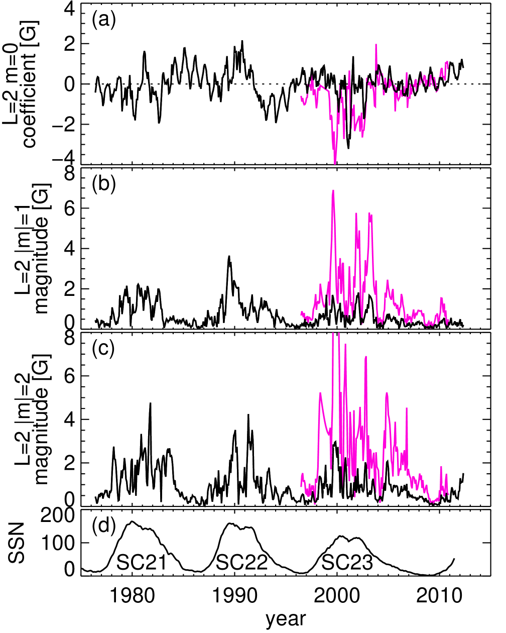
Figure 5: Evolution of the quadrupolar ($\ell=2$) modes, as characterized by the (a) axial quadrupole coefficient $B_{2}^{0}$, along with higher-order magnitudes of the (b) $m=\pm 1$ modes $\sqrt{(B_{2}^{-1})^{2}+(B_{2}^{1})^{2}}$ and (c) $m=\pm 2$ modes $\sqrt{(B_{2}^{-2})^{2}+(B_{2}^{2})^{2}}$, for the WSO (black) and MDI polar-corrected (magenta) data sets. Panel (d) shows the monthly smoothed SSN. The WSO data have not been corrected for known saturation effects that reduce the reported values by a factor of 1.8 (Svalgaard et al. 1978).

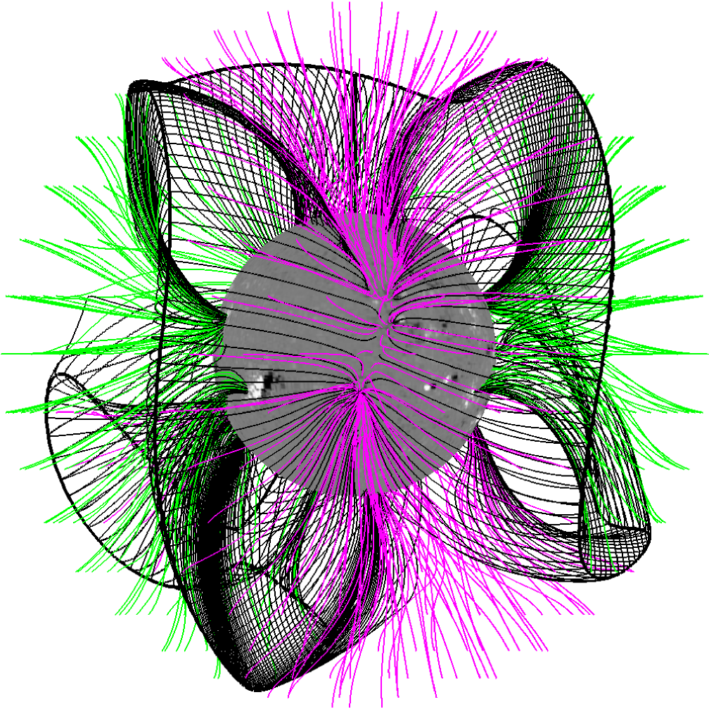
Figure 6: Representation of the coronal magnetic field in October 2000 for which the large-scale field is predominantly quadrupolar. This field is the result of a potential-field source-surface extrapolation (Schatten et al. 1969) with an upper boundary of 2.5 $R_{\odot}$ at which the coronal field is assumed purely radial. Both closed (black) and open (magenta and green, depending on polarity) field lines are shown in the model. Also shown is the contour of $B_{r}=0$ at $R=2.5R_{\odot}$ (thicker black line).

3.4 Octupole Field (Modes with $\boldsymbol{\ell}=3$)

As with the quadrupole, the octupolar modes contain more power during periods of high activity and less power during minimum conditions, as illustrated in Figure 7. The exception is the axial octupolar coefficient $B_{3}^{0}$, plotted in panel (a) of Figure 7, which is nonzero during solar minima and exhibits sign reversals during sunspot maxima in a manner similar to the axial dipole coefficient $B_{1}^{0}$.

The behavior of the various $m=0$ modes can be understood by considering their functional symmetry: the $Y_{\ell}^{0}$ functions are antisymmetric in $\theta$ (i.e., antisymmetric across the equator) when the degree $\ell$ is odd, whereas for even $\ell$ the $Y_{\ell}^{0}$ functions are symmetric in $\theta$. The presence of polar caps during solar minimum, a highly antisymmetric configuration, is reflected in the similar evolution of the $B_{1}^{0}$ and $B_{3}^{0}$ coefficients, which correspond to the axial dipole ($\ell=1$, $m=0$) and octupole ($\ell=3$, $m=0$) modes. The axial quadrupole ($\ell=2$, $m=0$) mode does not share this behavior because, as a symmetric mode, it is not sensitive to the presence of the polar caps during solar minima.

The dependence of the $B_{\ell}^{0}$ coefficients on the degree $\ell$ is illustrated in Figure 8, where the time-averaged energies from the MDI data (spanning Solar Cycle 23) as a function of degree $\ell$ are plotted. Prior to averaging, the spectra were placed in two classes: Carrington rotations for which the SSN is relatively large (defined as when SSN>100) and rotations for which the SSN is relatively small (defined as when SSN<50), thus capturing the state of the Sun when it is either overtly active or overtly quiet. The figure indicates that the even-odd behavior is more pronounced during quiet periods, and these occur near and during solar minimum when the polar-cap field is significant. During active periods the even-odd trend is still recognizable, but because the polar caps are weak and the active regions are primarily oriented east-west (i.e., in the equatorial plane and thus contributing little power to the axisymmetric modes) the even-odd trend is less pronounced. We will further discuss the behavior of axisymmetric modes in the context of Babcock-Leighton dynamo models in Section 4.2.

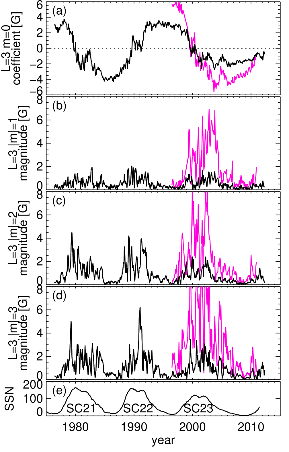
Figure 7: Evolution of the octupolar ($\ell=3$) modes, as characterized by the (a) axial octupole coefficient $B_{3}^{0}$, along with higher-order magnitudes of the (b) $m=\pm 1$ modes $\sqrt{(B_{3}^{-1})^{2}+(B_{3}^{1})^{2}}$, (c) $m=\pm 2$ modes $\sqrt{(B_{3}^{-2})^{2}+(B_{3}^{2})^{2}}$, and (d) $m=\pm 3$ modes $\sqrt{(B_{3}^{-3})^{2}+(B_{3}^{3})^{2}}$, for the WSO (black) and MDI polar-corrected (magenta) data sets. Panel (e) shows the monthly smoothed SSN. The WSO data have not been corrected for known saturation effects that reduce the reported values by a factor of 1.8 (Svalgaard et al. 1978).

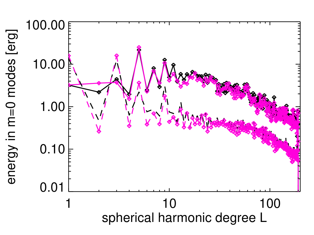
Figure 8: Time-averaged energies in the axisymmetric modes $\overline{(B_{\ell}^{0})^{2}}$ as a function of $\ell$ for MDI original (black) and polar-corrected (magenta) data sets, for more active conditions (solid lines; defined as when SSN>100) and for quieter periods (dashed lines; defined as when SSN<50). The interpolation scheme used to correct the MDI polar flux is described in Sun et al. (2011).

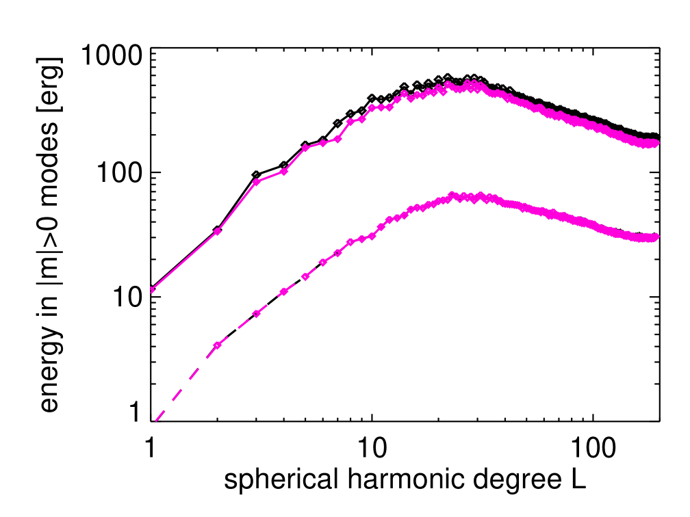
Figure 9: Time-averaged energies in the non-axisymmetric modes $\overline{\sum_{m>0}(B_{\ell}^{m})^{2}}$ as a function of $\ell$ for MDI original (black) and polar-corrected (magenta) data sets, for more active conditions (solid lines; defined as when SSN>100) and for quieter periods (dashed lines; defined as when SSN<50). The interpolation scheme used to correct the MDI polar flux is described in Sun et al. (2011).

3.5 Full Spectra and Most Energetic Modes

One property of the spherical harmonic functions $Y_{\ell}^{m}(\theta,\phi)$ is that the degree $\ell$ is equal to the number of node lines (i.e., contours in $\theta$ and $\phi$ where $Y_{\ell}^{m}=0$). In other words, the spatial scale represented by any harmonic mode (i.e., the distance between neighboring node lines) is determined by its spherical harmonic degree $\ell$. As a result, the range of $\ell$ values containing the greatest amount of energy indicates the dominant spatial scales of the magnetic field.

To this end, we have averaged the non-axisymmetric power spectra from each of the datasets both over time and over $m$, and have displayed the result in Figure 9. As with Figure 8, we have divided the spectra into active and quiet classes depending on SSN. In the figure, it can be seen that the magnetic power spectra form a broad peak with a maximum degree occurring at $\ell_{P_{\text{max}}}\approx$25, corresponding to a size scale of about 360${}^{\circ}/\ell_{P_{\text{max}}}\approx$15^∘ in heliographic coordinates. Stated another way, this indicates that much of the magnetic energy can be found (not surprisingly) on the spatial scales of solar active regions or their decay products.

Energy spectra determined from WSO charts (not shown) do not show the same broad peak at $\ell_{P_{\text{max}}}\approx$25 as found in the curves from the MDI-derived data shown in Figure 9. This is an effect of the lower spatial resolution of the WSO magnetograph (which has 180$\arcsec$ pixels, and is stepped by 90$\arcsec$ in the east-west direction and 180$\arcsec$ in the north-south direction when constructing a magnetogram) versus MDI (which has a plate scale of 2$\arcsec$ per pixel in full-disk mode). The WSO magnetograph, as a result, does not adequately resolve modes higher than about $\ell=15$, creating aliasing effects even at moderate values of $\ell$ in the energy spectra. Accordingly, as longer time series of data from newer, higher-resolution magnetograph instrumentation are assembled, the high-$\ell$ behavior of the energy spectra (such as those shown in Figs. 8 and 9) may change due to better observations of finer scales of magnetic field.

3.6 Primary and Secondary Families

The projection of the solar surface magnetic fields onto spherical harmonic degrees allows us to delineate the main symmetries of the magnetic field. As noted in §2, the harmonic modes can be classified as either axisymmetric ($m=0$) or non-axisymmetric ($m\neq 0$). Separately, the harmonic modes can be either antisymmetric (odd $\ell+m$) or symmetric (even $\ell+m$) with respect to the equator (Gubbins & Zhang 1993). Some authors refer to antisymmetric modes as dipolar and symmetric modes as quadrupolar (presumably because the axial dipole and quadrupole modes usually possess the most power in their respective categories), while others synonymously assign these modes to either the primary and secondary family (e.g., McFadden et al. 1991 when characterizing the Earth’s magnetic field geometry), respectively. In this article, we adopt the primary- and secondary-family nomenclature when describing the equatorial symmetry because this avoids the confusion that may otherwise occur when, for example, it is realized that the equatorial dipole mode ($\ell=1,m=1$) formally belongs to the “quadrupolar” family of modes (since $\ell+m$ is even for this mode).

One important result put forward by the geomagnetic community is that the relative strengths of the primary and secondary families are different during geomagnetic field reversals and excursions. During reversals, the modes associated with the secondary family predominate over primary-family modes, and during excursions this is not the case (Leonhardt & Fabian 2007). We now investigate whether analogous behavior is occurring in the solar setting, by determining which harmonic modes are most correlated with the axial dipole and axial quadrupole.

When applied to two variables, the Spearman rank correlation index $\rho\in[-1,1]$ indicates the degree to which two variables are monotonically related. The index $\rho$ is positive when both variables tend to increase and decrease at the same points in time. A rank correlation analysis is more general than a more common Pearson correlation analysis, which specifically measures how well two variables are linearly related, whereas the rank correlation analysis enables a determination of whether the time evolution of two mode amplitudes follow a similar pattern in time without regard to their (unknown) functional dependency.

In Table 1 we list the degrees $\ell$ and orders $m$ corresponding to the harmonic coefficients $B_{\ell}^{m}(t)$ that have the highest $\rho$ (positive correlation) when compared with the axial dipole and axial quadrupole coefficients $B_{1}^{0}(t)$ and $B_{2}^{0}(t)$ (which peak at different phases of the sunspot cycle). The corresponding harmonic modes comprise the strongest modes in the primary and secondary families, respectively. We find that, among the mode amplitudes that are positively correlated with $B_{1}^{0}$, two out of three belong to the primary family. Similarly, for $B_{2}^{0}$, 7 of the 10 most-correlated modes are members of the secondary family.

These correlations indicate a preference in the solar dynamo, at least as inferred from its surface characteristics, for modes belonging to the same family and thus having the same north-south symmetry characteristics to be excited nearly in phase. This preference is demonstrated further in Figures 10 and 11, in which the long-term trends of the time evolution of the first several axisymmetric mode coefficients are shown, after smoothing with a boxcar filter having a width of 1 yr. (We focus here on the axisymmetric mode properties because these modes are the only ones considered in most mean-field dynamo models, as discussed further in §4.2.) In Figure 10, there is a clear correlation amongst the first few odd-$\ell$ and amongst the first couple of even-$\ell$ mode coefficients, a trend which is emphasized in Figure 11 in which these same mode coefficients are overplotted. We note that the mode groupings are not precisely in phase, as evidenced for example by the lag in $\ell=3$ and especially the $\ell=5$ modes reversing signs with respect to the $\ell=1$ mode. When $\ell\geq 6$ or so, these trends become much weaker amongst the axisymmetric modes (although Table 1 indicates that this is not necessarily true for the non-axisymmetric modes), presumably because as smaller and smalle1r scales are considered the effects of the global organization associated with the 11-year sunspot cycle are less important in structuring the surface magnetic field.

Figure 11 additionally illustrates that the modes of the secondary family attain amplitudes of about 25% of the primary mode amplitudes. Furthermore, the primary and secondary mode families are out of phase: during reversals the primary modes become weak at the same time as the amplitudes of the modes associated with the secondary family become maximal, which was shown previously in Figure 4(c). This same pattern is observed to occur during reversals of the axial dipole field of the geodynamo. As in the geodynamo case, we ascribe the relative amplitudes and phase relation between the primary and secondary families observed during solar dipole reversals as a strong indication that the interplay of the mode families play a key role in the process by which the axial dipole reverses. Hence, any realistic model of the solar dynamo must excite both families of modes to similar amplitude levels, and must exhibit similar coupling between modes belonging to the primary and secondary families.

Most Correlated modes

	$\ell=1$, $m=0$			$\ell=2$, $m=0$
$\ell$	$m$	Primary	$\ell$	$m$	Secondary
3	0	Y	4	0	Y
5	0	Y	4	1	N
2	0	N	9	9	Y
			6	1	N
			7	0	N
			9	1	Y
			5	1	Y
			1	1	Y
			7	7	Y
			3	3	Y

Table 1: Ranking of the most positively correlated modes within the primary and secondary families for which $\ell\leq 9$. The basis for comparison in each family is the lowest-degree axisymmetric mode belonging to each family, specifically the axial dipole ($\ell=1$, $m=0$) and axial quadrupole ($\ell=2$, $m=0$) modes for the primary and secondary families, respectively. The most correlated mode is the next axisymmetric mode in each family. The equatorial dipole mode ($\ell=1$, $m=1$) is more correlated with the axisymmetric quadrupole, as expected from its symmetry properties. We note the presence of 4 sectoral modes (for which $\ell=m$) in the list of the secondary family.

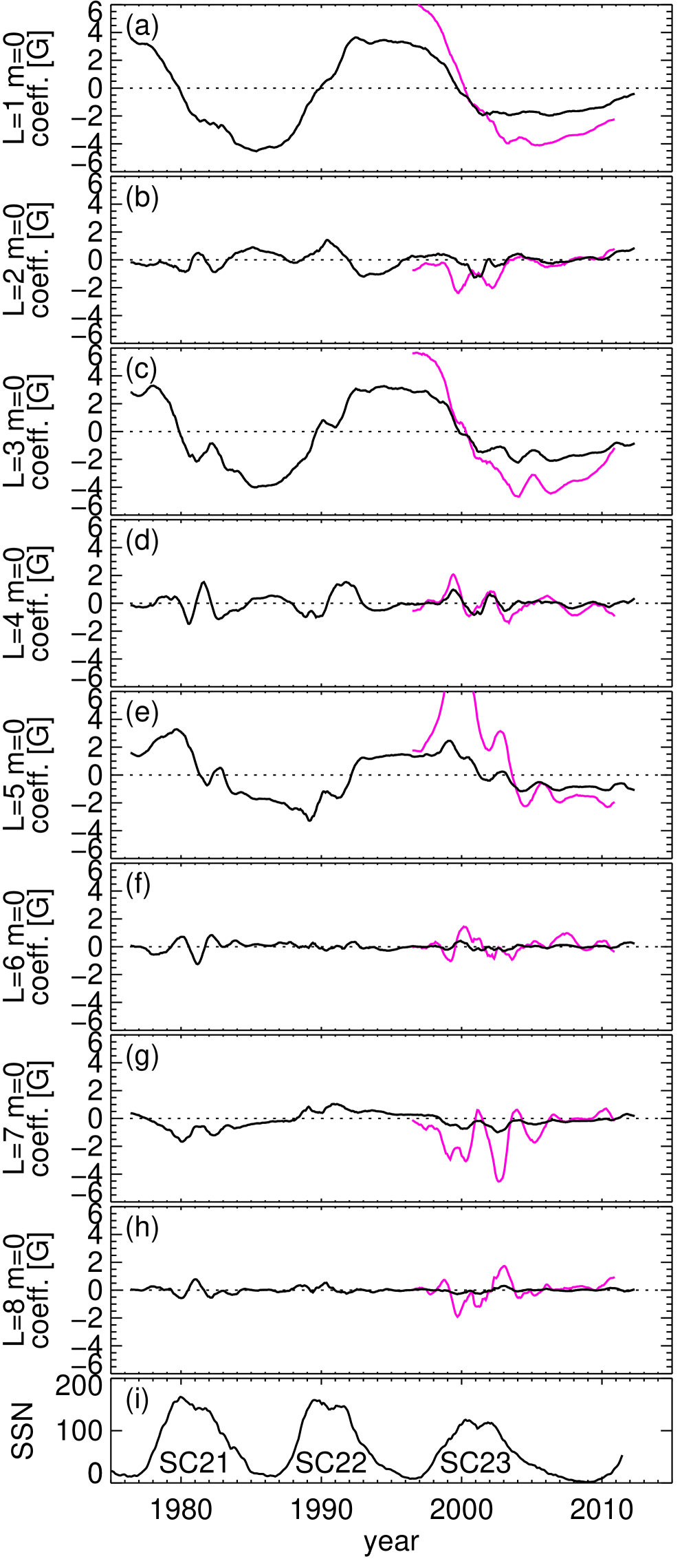
Figure 10: (a)–(h) Coefficients $B_{\ell}^{0}$ for the axisymmetric modes of the first eight degrees $\ell$ as a function of time, as calculated from the WSO (black) and MDI polar-corrected (magenta) synoptic maps and after boxcar smoothing with a width of 1 yr. Panel (i) shows the monthly smoothed SSN. The WSO data have not been corrected for known saturation effects that reduce the reported values by a factor of 1.8 (Svalgaard et al. 1978).

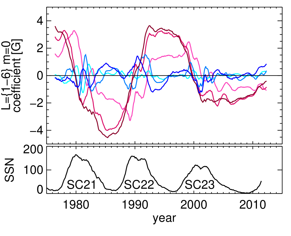
Figure 11: Overplotted coefficients $B_{\ell}^{0}$ from Figure 10 of the first 3 odd ($\ell=\{1,3,5\}$; dark red, red, light red lines, respectively) and even ($\ell=\{2,4,6\}$; dark blue, blue, light blue, respectively) axisymmetric modes, as calculated from WSO synoptic maps.

4 Theoretical Implications for Solar Dynamo

As demonstrated in previous sections, the amplitudes of the various harmonic modes of the solar magnetic field are continually changing. During reversals, as the axial dipole necessarily undergoes a change in sign, other modes predominate such that the amplitude of the solar magnetic field never vanishes during a reversal. As a result of such reversals occurring in the middle of each 11-yr sunspot cycle, during the rising phase of each cycle the polar fields and the emergent poloidal fields have opposite polarity (Babcock 1961; Benevolenskaya 2004), while in the declining phase the polarity of sunspots and active regions are aligned with the newly formed polar-cap field.

We have already noted how the temporal modulation of the large-scale harmonic modes comprising the primary and secondary families during polarity reversals appears similar to that of the magnetic field of the Earth (McFadden et al. 1991; Leonhardt & Fabian 2007). We have illustrated that as the magnitude of the primary-family mode amplitudes (primarily those of the axisymmetric odd-$\ell$ modes $B_{\ell}^{0}$) lessen, the secondary-family mode amplitudes (particularly those of the equatorial dipole $B_{1}^{1}$ and axial quadrupole $B_{2}^{0}$) simultaneously increase. Once the secondary-family modes have peaked, the primary-family modes grow as a result of the growing polar-caps. Such interplay between primary and secondary families provides insight toward an understanding of the processes at play in the solar dynamo that are assumed to be responsible for the occurrence of the observed cyclic activity (Tobias 2002).

The presence of power in members of both the primary and secondary families indicates that the solar dynamo excites modes that are both symmetric and antisymmetric with respect to the equator. As was demonstrated by Roberts & Stix (1972), this cannot occur unless nonlinearities exist or unless basic ingredients of the solar dynamo (such as, for example the $\alpha$ and/or $\omega$ effects, or the meridional flow) possess some degree of north-south asymmetry. In light of the the parameter regime in which the solar dynamo is thought to operate, including large fluid and magnetic Reynolds numbers $R_{e}$ and $R_{m}$ believed to characterize the solar convection zone (both of order $10^{12}$–$10^{15}$; Stix 2002; Ossendrijver 2003), one expects the Sun to possess a nonlinear dynamo. Detailed observations of the magnetic field in the solar interior where dynamo activity is thought to occur are not available, but the observed magnetic patterns and evolution provide circumstantial evidence of turbulent, highly nonlinear processes that lead to complex local and nonlocal cascades of energy and magnetic helicity (Alexakis et al. 2005, 2007; Livermore et al. 2010; Strugarek et al. 2012). Yet, the presence of regular patterns formed by the emergent flux on the solar photosphere, as codified by Hale’s Polarity Law, Joy’s Law for active-region tilts, and the approximately regular cycle lengths, suggest that some ordering is indeed happening in the solar interior.

With the aim of distilling the necessary elements of the various nonlinear dynamos into a manageable framework, multiple authors have created idealized models of the solar dynamo, including (for example) Weiss et al. (1984); Feynman & Gabriel (1990); Ruzmaikin et al. (1992); Knobloch & Landsberg (1996); Tobias (1997); Knobloch et al. (1998); Melbourne et al. (2001); Weiss & Tobias (2000); Spiegel (2009). Similarly, for the geodynamo there are many efforts, including Glatzmaier & Roberts (1995); Heimpel et al. (2005); Christensen & Aubert (2006); Busse & Simitev (2008); Nishikawa & Kusano (2008); Takahashi et al. (2008); Christensen et al. (2010). A completely different approach has been taken by Pétrélis & Fauve (2008) and Pétrélis et al. (2009), who have developed simplified models of the von Karman sodium (VKS) laboratory experiment (Monchaux et al. 2007). In all of these idealized models, the modulations resulting from the coupling between magnetic modes from the different families, or between the magnetic field and fluid motions (Tobias 2002) can be analyzed in terms of the equations that describe the underlying systems. The variability of the most prominent cycle period develops as a result of the coupling of modes introducing a second time scale into the dynamo system, often leading to a quasi-periodic or chaotic behavior of the magnetic field, cycle length, and/or dominant parity. One can further understand via symmetry considerations how reversals and excursions arise (Gubbins & Zhang 1993).

4.1 Reversals and Coupling between Modes

To illustrate such a dynamical system, following the work of Pétrélis & Fauve (2008), we assume that the axial dipole and quadrupole modes are nonlinearly coupled. We can then define a variable $A(t)=B_{1}^{0}(t)+iB_{2}^{0}(t)$, where we have used the time-varying mode coefficients defined in Equation 1, and write an evolution equation that satisfies the symmetry invariance found in the induction equation, i.e., $\boldsymbol{B}\rightarrow-\boldsymbol{B}$. It then follows that the symmetry $A\rightarrow-A$ must also be satisfied, and that such a equation to leading order is

$$\frac{dA}{dt}=\mu_{1}A+\mu_{2}\bar{A}+\nu_{1}A^{3}+\nu_{2}A^{2}\bar{A}+\nu_{3}A\bar{A}^{2}+\nu_{4}\bar{A}^{3},$$ (5)

where $\mu_{i}$ and $\nu_{i}$ are complex coefficients and $\bar{A}=B_{1}^{0}-iB_{2}^{0}$ is the complex conjugate of $A$, and the quadratic terms have vanished due to symmetry considerations. As discussed in Pétrélis & Fauve (2008) and Pétrélis et al. (2009), such dynamical systems are subject to bifurcations. In particular, they demonstrate that this dynamical system can be characterized by a saddle-node bifurcation when comparing its properties with so-called normal form equations (Guckenheimer & Holmes 1982). In such a bifurcated system, both stable and unstable equilibria (fixed points) exist, as illustrated in the left panel of Figure 12. For instance, if the solution lies at a stable point (for example, where the dipole axis is oriented northward), fluctuations in the system may disturb the equilibrium and push the magnetic axis away from its stable location. If such fluctuations are not strong enough, the evolution of the dynamical system resists the deterministic evolution of the system and the system returns to its original configuration (in the example, resulting in an excursion of the dipole), such as seen in the geomagnetic field (Leonhardt & Fabian 2007). If instead the fluctuations are large enough to push the system past the unstable point, the magnetic field then evolves toward the opposite stable fixed point allowed by $\boldsymbol{B}\rightarrow-\boldsymbol{B}$ (in the example, resulting in a reversal that changes the dipole axis to a southward orientation). Such behavior is also seen in the VKS experiment, from which is observed irregular magnetic activity combined with both excursions and reversals. Reversals result in an asymmetric temporal profile, with the dipole evolving slowly away from its equilibrium followed by a swift flip (cf., Fig. 3 of Pétrélis et al. 2009).

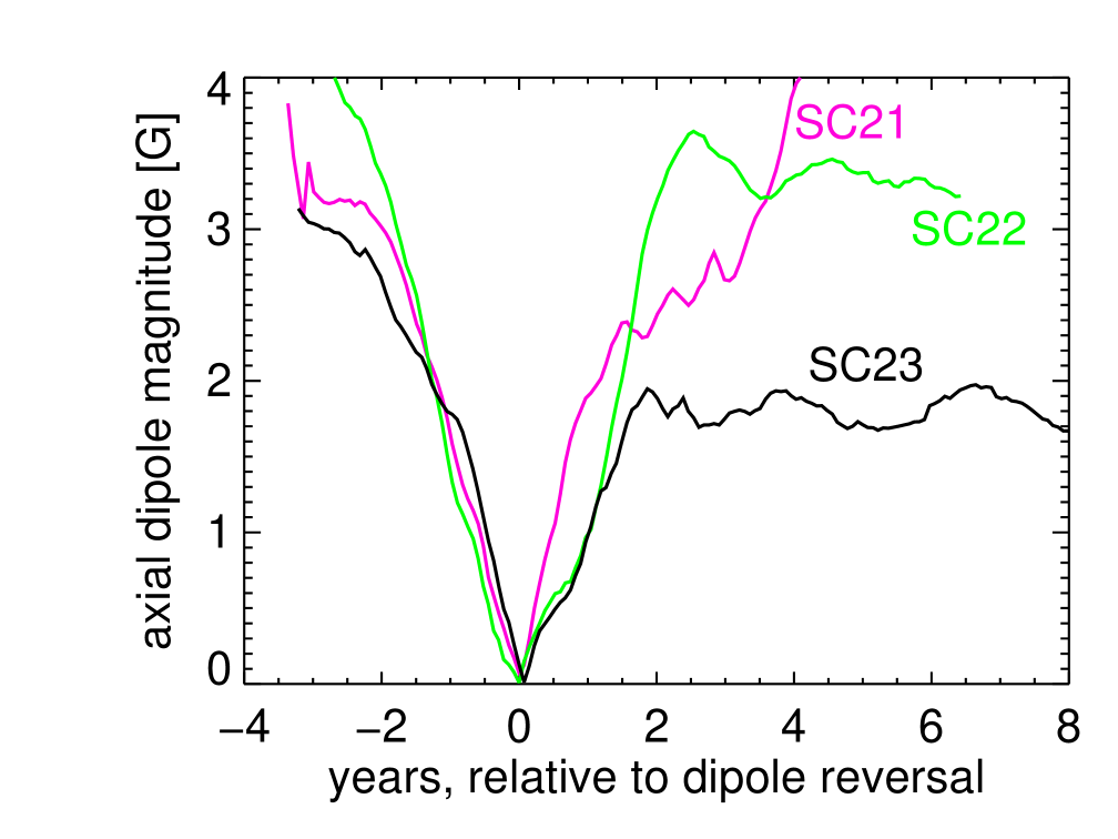
Figure 13: The reversals, as defined by the magnitude of the axial dipole component for WSO, for the past sunspot Cycles 21–23. The reversal for these three cycles occurred in Oct. 1979, Nov. 1989, and Jul. 1999, respectively.

In Figure 13 we have overplotted the last three sunspot cycle reversals such that the zero-crossings of the axial dipole coefficients $B_{1}^{0}$ for each cycle are aligned. It has been recently shown that the 10 major geomagnetic reversals for which detailed records exist occurring during the past 180 Myr possess a characteristic shape upon suitable normalization (Valet & Fournier 2012). This shape can be described as comprising a precursory event lasting of order 2500 yr, a quick reversal not exceeding 1000 yr, and a rebound event of order 2500 yr. Pétrélis et al. (2009) show that the magnetic field in a simplified VKS laboratory experiment exhibits differing behavior during reversals and excursions. During reversals, the magnetic field has an asymmetric profile that contains a slow decrease in the dipole, followed by a rapid change of polarity and buildup of the opposite polarity, whereas excursions are more symmetric. Additionally, after reversals the magnetic dipole overshoots its eventual value before settling down, whereas during excursions no such overshooting is measured (see Fig. 3 of Pétrélis et al. 2009). For the solar cases displayed in Figure 13, we find that only the (green) curve of the reversal of cycle 22 exhibits an overshoot, whereas the other two cycles do not. Further, the rates at which the solar dynamo approaches and recovers from the reversal appear to be equal, leading to a symmetric profile, in contrast with the VKS results. Therefore, the Sun seems to reverse its magnetic field in a less systematic way than other systems that have shown such behavior.

Analyzing such systems from a dynamical systems perspective, when changing the control parameter (here, $R_{m}$) past the bifurcation point, the stable and unstable points coalesce and merge and the saddle nodes disappear, as shown in the right panel of Figure 12. This act transforms the system from one containing fixed points to one containing limit cycles with no equilibria (e.g., Guckenheimer & Holmes 1982), yielding an oscillatory solution that manifests itself as cyclic magnetic activity. Typically, large fluctuations are required in order to put the dynamical system above the saddle-node bifurcation threshold.

In the case of the Sun, both the primary and secondary families are excited efficiently and a strong coupling between them is exhibited. The model of Pétrélis & Fauve (2008), in spirit very close to the studies of Knobloch & Landsberg (1996) or Melbourne et al. (2001), may be used to guide our interpretation of the solar data. As illustrated in Figure 11, the axisymmetric dipole and quadrupole are out of phase, such that their coupling may lead to global reversals of the solar poloidal field. To the best of our knowledge, however, the solar dynamo does not exhibit excursions of its magnetic field (unlike the geodynamo) but instead undergoes fairly regular reversals that take about one or two years to transpire (cf., Fig. 3). The solar dynamo is thus better approximated by a model in which a limit cycle is present. One may presume that the difference between the geodynamo and the solar dynamo may be a result of the large degree of turbulence present in the solar convection zone, whereas the mantle of the Earth has a more laminar convective flow and thus is below the bifurcation threshold where fixed points are still present.

It may be the case that the solar dynamo is better described by a Hopf bifurcation, in which a limit cycle arises (branches from a fixed point) as the bifurcation parameter is changed. The dynamo instability that occurs as a result of the interaction of magnetic fields and fluid flows (such as $\alpha\omega$ dynamos typically used to model the Sun, as summarized in Tobias 2002) often arises from a Hopf bifurcation. This allows the system to pass through domains having different properties, such as the aperiodic oscillations that characterize the grand minima and nonuniform sunspot cycle strengths of the solar dynamo (e.g., Spiegel 2009 and references therein). The data analysis shown here does not favor a particular type of bifurcation, but does indicate efficient coupling between the primary and secondary families.

Yet another approach toward investigating magnetic reversals is to develop detailed numerical simulations solving the full set of MHD equations. Such three-dimensional numerical simulations in spherical geometry of the Earth’s geodynamo (Glatzmaier & Roberts 1995; Li et al. 2002; Nishikawa & Kusano 2008; Olson et al. 2011) or of the solar global dynamo (Brun et al. 2004; Browning et al. 2006; Racine et al. 2011) have looked at the behavior of the polar dipole vs multipolar modes. Even though such models have large numerical resolution and thus possess a large number of modes, all have the property that the dominant polarity of the magnetic field follows the temporal evolution of a few low-order modes, even if in some cases the magnetic energy spectrum peaks at higher angular degree $\ell$. These findings suggest that the coupling between the primary and secondary family remains an important factor in characterizing polarity reversals for these simulations, and is thought to be linked to a symmetry-breaking of the convective flow (Nishikawa & Kusano 2008; Olson et al. 2011). Some studies of the geomagnetic field (e.g., Clement 2004) even advocate for a coupling between two modes of the same primary family, such as the axial dipole and octupole. While in the solar data these modes are well correlated, the coupling between the primary and secondary families of modes seems more likely to be at the origin of the reversal, as demonstrated in §3.6.

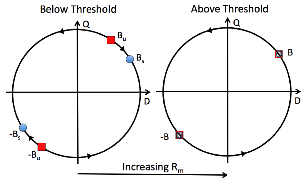
Figure 12: Schematic diagrams (adapted from Pétrélis et al. 2009) of a magnetic dynamo system on either side of a saddle-node bifurcation, with two distinct polarity configurations represented by $B$ and $-B$. The coordinate axes represent states where the primary (as represented by the axial dipole $D$) or secondary (as represented by the axial quadrupole $Q$) families are dominant. In the left-hand diagram, stable ($\pm B_{s}$) and unstable ($\pm B_{u}$) states present during the system’s evolution are indicated by blue circles and red squares. Perturbations away from a stable point can either cause the system to evolve to the opposite stable configuration (if the perturbation is strong enough) or simply cause an excursion in which the system returns to the same stable state. In the right-hand diagram, corresponding to the same system at a higher magnetic Reynolds number $R_{m}$ the stable and unstable points have merged, and the system simply oscillates between the two configurations in a limit cycle.

4.2 Mean-Field Dynamo Models and the Axisymmetric Modes

Mean-field dynamo models are found to capture the essence of the large scale solar dynamo (Moffatt 1978; Ossendrijver 2003; Dikpati et al. 2004; Charbonneau 2010). At present, the most favored model is the mean-field Babcock-Leighton (BL) dynamo model (e.g., Dikpati et al. 2004), in which the mean magnetic induction equation is solved using empirical guidance for both the differential rotation and meridional circulation profiles, as well as for parameterizations of the $\alpha$-effect and poloidal-field source terms. In this section, we use the Stellar Elements (STELEM; T. Emonet & P. Charbonneau, 1998, priv. comm.) code (see Appendix A of Jouve & Brun 2007 for more details) to solve the axisymmetric BL dynamo equations, and investigate some of the consequences of the coupling between modes from the primary and secondary families. In the interest of brevity, we refer interested readers to Appendix A.1 for a listing of the governing equations associated with BL dynamos.

In many BL solar dynamo models, the parameters governing the imposed flows and the poloidal-field source terms are chosen based on their solar counterparts. When carefully chosen these terms favor modes from the primary family and thus antisymmetric field configurations, since this is what the Sun apparently favors much of the time. This is a result of the commonly used latitudinal profiles of the key dynamo ingredients (symmetric large-scale flows and antisymmetric alpha effect) combined with the parity in the BL mean-field dynamo equations, leading to a situation where modes of the primary family remain uncoupled to modes of the secondary family that allows both dynamo families to coexist without much interaction. We consider the symmetry of the BL equations used here in Appendix A.2 (see also Roberts & Stix 1972 and Gubbins & Zhang 1993 for broader discussions on this topic).

To demonstrate these characteristics, we now consider a typical solution of the standard BL mean-field dynamo as calculated by STELEM. Figure 14 presents the time evolution of the resulting magnetic field patterns, and is thus analogous to the standard solar butterfly diagram. Performing a Legendre transform on the magnetic field reveals the degrees $\ell$ of the dominant axisymmetric modes. Figure 15 illustrates that the odd $\ell$ modes from the primary family dominate over the even ones by about five orders of magnitude in this model. This differs significantly from what is observed on the Sun, where the amplitude of the quadrupole is measured to be about 25% of the dipole amplitude for most of the time, becoming dominant only during reversals [cf., Fig. 4(c)]. The behavior of the standard BL model of Figure 15 arises because of the symmetry characteristics of the BL dynamo equations. Because the model was initialized with a dipolar field, no modes from the secondary family are excited in the standard BL model shown in Figure 15 because no coupling exists between the primary and secondary families.

If instead the calculation were initialized with a quadrupolar field (belonging to the secondary family), we find that the system eventually transitions to a state in which the primary-family modes predominate, as shown in Figure 16. The growth of the primary-family modes is due to the presence of a very weak dipole (likely of numerical origin) at the onset of the simulations. In these models, the BL source term of Equation (A8) quenches the growth of the magnetic field once a certain threshold is passed, and as a result the maximum total amplitude of the magnetic field is capped. The reason why the primary-family modes are preferred stems from the fact that the thresholds for dynamo action (based on the parameter $C_{s}$ in Equation [A4]) are found empirically to be lower for the dipole than for the quadrupole ($C_{s}\sim 6.12$ vs. $C_{s}\sim 6.25$), meaning the dipole-like modes have a higher growth rate than the quadrupole-like modes. In this model, only briefly during the transition phase does the model possess a quadrupole of order 25% of the dipole, as in the Sun.

Observations of solar photospheric fields, however, indicate that the Sun excites both families and does not strongly favor members of one family over the other, a situation that has apparently existed over many centuries. Even during the Maunder minimum, evidence suggests that this interval may have been dominated by a hemispherical dynamo with magnetic activity located primarily in the southern hemisphere (Ribes & Nesme-Ribes 1993), which can only be formed by a state in which primary- and secondary-family modes possess nearly equal amplitudes (Tobias 1997; Gallet & Pétrélis 2009). Consequently, the solutions presented in Figures 15 and 16, in which modes from only one family are preferred, are thus not a satisfactory model of the Sun.

As advocated by Roberts & Stix (1972) and Gubbins & Zhang (1993) following their symmetry-based study of the solar dynamo and the induction equation, and more recently by Nishikawa & Kusano (2008) in their geodynamo simulations, a north-south asymmetry of the flow field specified in the BL dynamo, or alternatively an asymmetric poloidal-field source term, may allow the co-existence of both the primary and secondary families. To investigate this effect we have performed two additional BL dynamo calculations, one with a BL source term and one with a meridional circulation that each generate both symmetric and antisymmetric fields (introduced via the parameter $\epsilon$ of Equations (A9) and (A13) of Appendix A.1), the combination of which yields asymmetric magnetic field patterns.

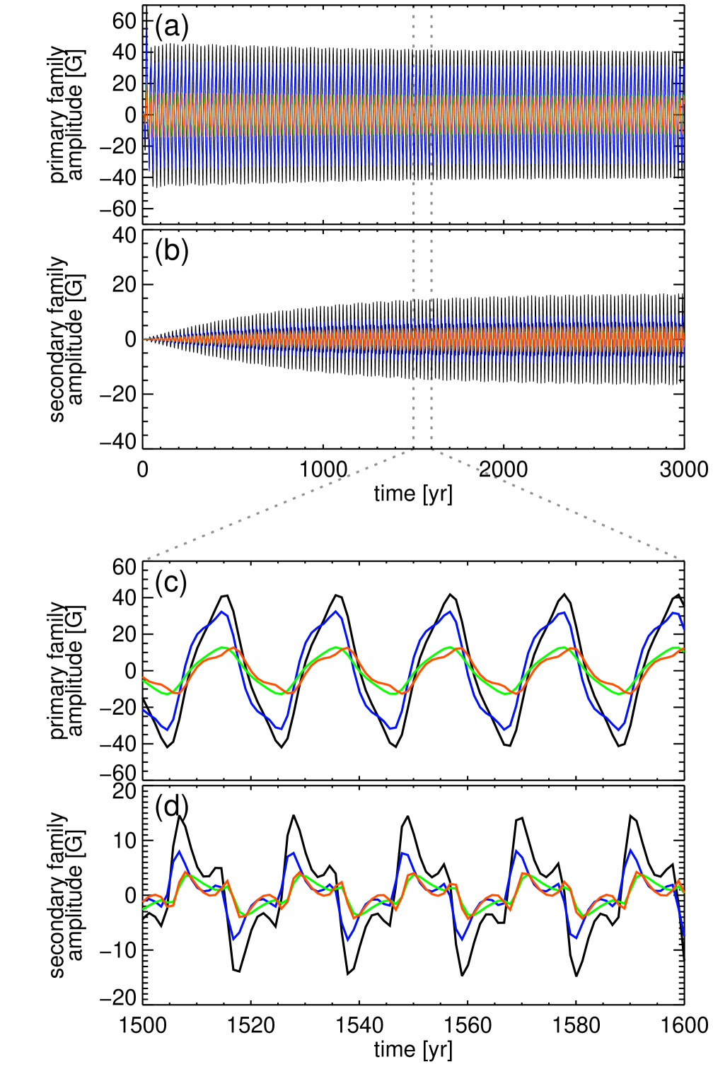
Figure 18: Time evolution of the same BL model as shown in Fig. 15 (and using the same color scheme), but with an asymmetric meridional flow profile as implemented in Eq. (A13) by setting $\epsilon=10^{-3}$.

We have run several dynamo cases, with the antisymmetry arising either in the BL source term or in the meridional flow profile, and with a range of amplitudes for the $\epsilon$ parameter from $10^{-4}$ to $10^{-1}$. All cases were initialized with a dipolar field. We find that when $\epsilon$ is about $10^{-3}$, the modes in secondary family grow until they reach about 35% of the dominant dipolar mode, as illustrated in Figures 17 and 18. This result holds true regardless of whether the antisymmetry is introduced in the BL source term or in the meridional circulation profile, with very little difference in the resulting mode amplitudes. As expected, using a smaller $\epsilon$ results in solutions where the primary-family modes dominate, while using a larger $\epsilon$ yields a state where the secondary-family modes are comparable to the primary-family modes. Such results may indicate that Sun need only possess a weak degree of north-south asymmetry in order to behave as it does.

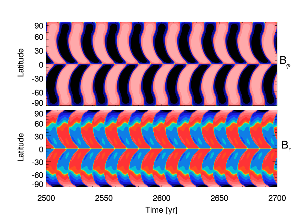
Figure 14: Latitude-time plots of $B_{\phi}$ (at the tachocline) and $B_{r}$ (at the surface) produced by a mean-field BL dynamo model that uses empirical guidance for the solar differential rotation and meridional flow profiles, and that is initialized with a dipolar magnetic field. The lower panel is analogous to the standard solar butterfly diagram.

5 Conclusions

Cycles of magnetic activity in many astrophysical bodies, including the Sun, Earth, and other stars, are thought to be excited by nonlinear interactions occurring in their interiors. Yet in some cases, such as the Sun, the cycles have approximately regular periods and in others, such as the Earth, there is no apparent periodicity. Dynamo theory indicates such a range of behaviors is expected, and whether the cycles are regular depends on magnetohydrodynamic parameters that characterize the system, including fluid and magnetic Reynolds and Rayleigh numbers. As a consequence, the large-scale appearance of the magnetic field may provide clues toward the type of dynamo that may be operating.

In this article, long-term measurements of the solar photospheric magnetic field are utilized to characterize the waves of dynamo activity that exist within the interior of the Sun. Synoptic maps from WSO (dating back to 1976) and MDI (spanning 1995–2010) are used to determine the spherical harmonic coefficients of the surface magnetic field for the past three sunspot cycles. We focus on the apparent interactions between various low-order modes throughout the past three sunspot cycles, and interpret these trends in the context of dynamo theory.

The multipolar expansions of the solar field as deduced from WSO and MDI data indicate that the axial and equatorial dipole modes are out of phase. During activity minima, the dipole component of the solar field is generally aligned with the axis of solar rotation, while the quadrupole component is much weaker. During activity maxima, the dipole reverses its polarity with respect to the rotation axis, and throughout the reversal process there is more energy in quadrupolar modes than in dipole modes. During the past three cycles, these reversals have taken place over a time interval of about 2 yr to 3 yr on average. More indirect measures of solar activity, such as the sunspot number and proxies of the heliospheric field, seem to indicate that such regular activity cycles have persisted for at least hundreds of years with a period of approximately 11 yr. The most recently completed solar cycle (Cycle 23) lasted for about 13 yr and while unusual, is not unprecedented. We note in passing that such modulations of the solar dynamo may be interpreted as a type of nonlinear interaction between the turbulent alpha effect and the field and/or flows (Tobias 2002).

The harmonic modes can also be grouped into primary and secondary families, a distinction that depends on the north-south symmetry of the various modes. For example, the axial dipole harmonic is antisymmetric and is a member of the primary family. Alternatively, the equatorial dipole and axial quadrupole modes are both symmetric with respect to the equator and thus are grouped together in the secondary family. When the evolution of the mode coefficients are analyzed in this way, we find that there is a trend for members of the same family to possess the same phasing, suggesting that modes in the same family of modes are either excited together and/or are more coupled when compared with modes of different families. This coupling is noticeable during reversals of the solar dipole, as less energy is present in primary-family modes than in secondary-family modes during these intervals.

The historical record indicates that the geodynamo also undergoes reversals of its dipole axis (with respect to the rotation axis), but these reversals occur much more irregularly than in the solar case. Additionally, the dipole axis of the terrestrial magnetic field occasionally makes excursions away from the axis of rotation of the Earth, only to later return without actually reversing. An examination of the large-scale harmonic modes of the geomagnetic field during these intervals indicates that the energy contained in secondary-family modes was significantly smaller during excursions than during reversals. A strong quadrupole during geodynamo reversals is in line with the solar behavior; there is no parallel with excursions as excursions in the solar case have not been observed. Analogous behavior is observed to occur in the VKS laboratory dynamo with respect to the relative strengths of the primary and secondary families.

We also examined the coupling of the mode families using a BL mean-field dynamo model computed using the STELEM code. Because of the symmetries in the magnetic induction and in the assumed profiles of the large-scale flow fields and BL source term, we find that the standard mean-field solar dynamo model results in a state containing largely members of the primary family. This is a result of the dipole (a primary-family mode) being more unstable to dynamo action than the quadrupole. With a modest amount of asymmetry, implemented here either in the meridional flow profile or in the BL source term, we find from the models that both the primary and secondary families can coexist in the same model and in the same proportions as in the solar dynamo. This can lead to a small lag between the northern and southern hemispheres as is actually observed on the Sun (Dikpati et al. 2007).

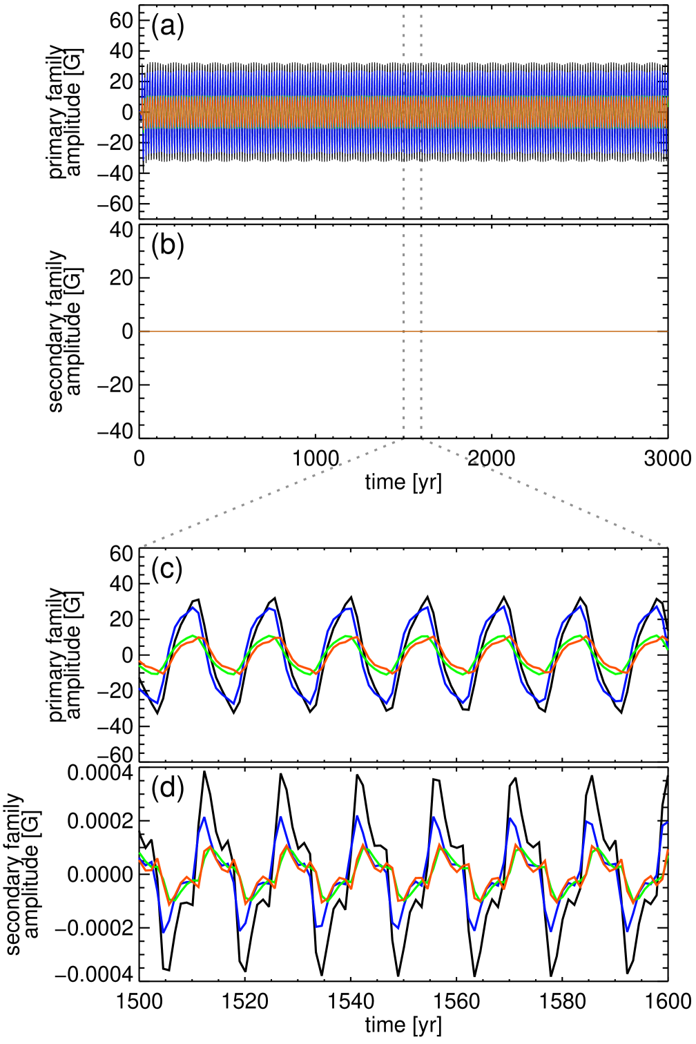
Figure 15: Time evolution of the coefficients of the lowest-order harmonic functions of the surface magnetic field (as grouped by primary and secondary families) from the same BL dynamo model as shown in Fig. 14. In panel (a) are shown the evolution of the first several primary-family coefficients $B_{\ell}^{0}$ with $\ell=$1, 3, 5, and 7 in black, blue, green, and red, respectively. In panel (b) are shown the evolution of the secondary-family coefficients $B_{\ell}^{0}$ with $\ell=$2, 4, 6, and 8, respectively in black, blue, green, and red. Panels (c) and  (d) show zoomed-in sections of panels (a) and (b).

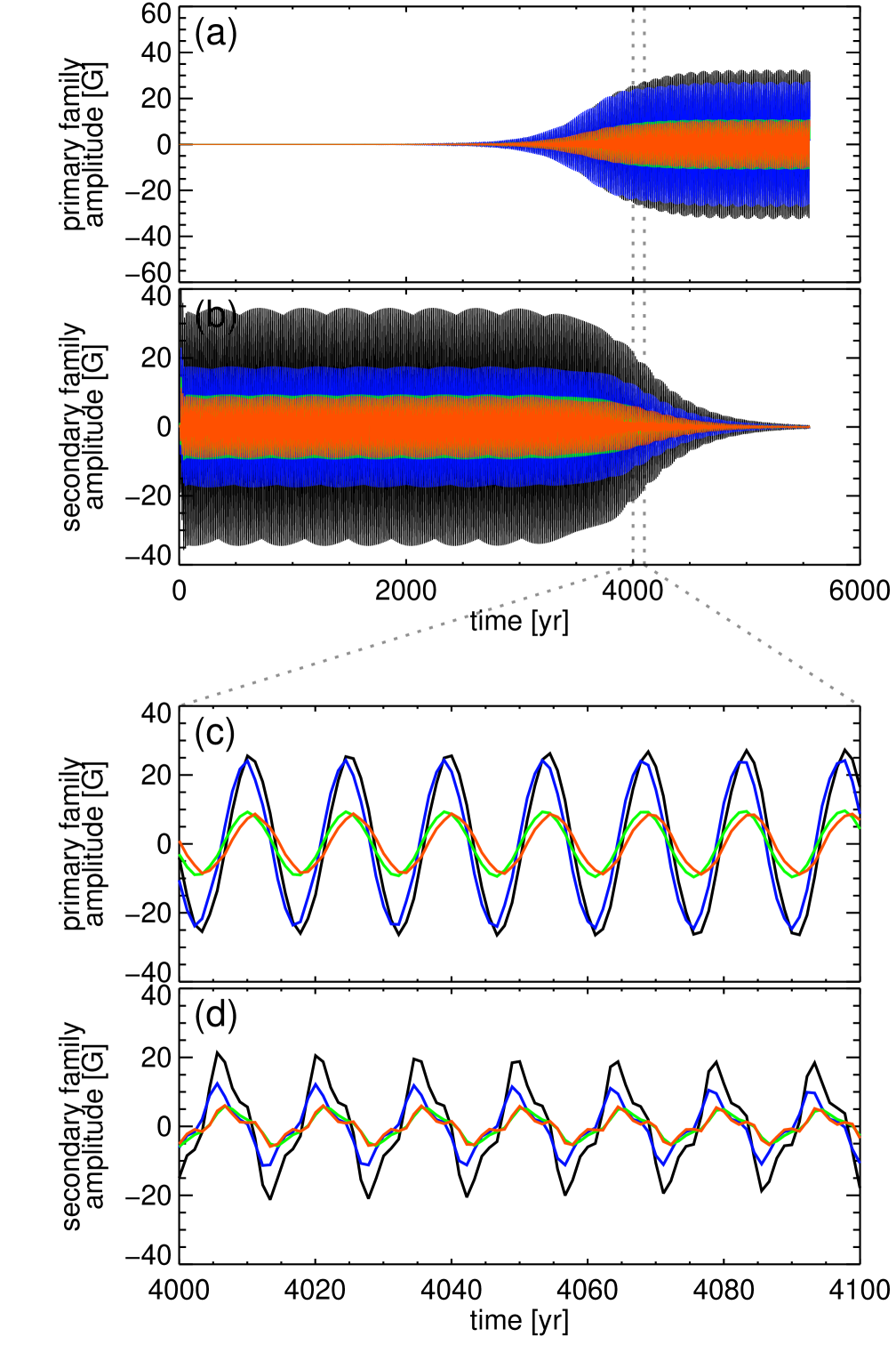
Figure 16: Time evolution of the same BL model as shown Fig. 15 (and using the same color scheme), but initialized with a quadrupolar magnetic field.

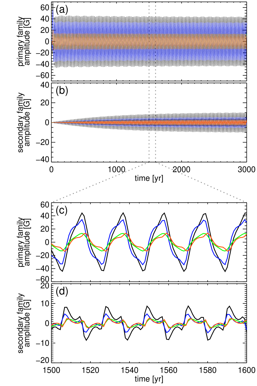
Figure 17: Time evolution of the same BL model as shown in Fig. 15 (and using the same color scheme), but with an asymmetric BL source term as implemented in Eq. (A9) by setting $\epsilon=10^{-3}$.

Appendix A Mean-Field Dynamo Formalism

In this Appendix, we provide details regarding the Babcock-Leighton mean-field dynamo models discussed in §4.2. The pertinent equations are listed in §A.1 and their symmetry properties are discussed in §A.2.

A.1 Mean-Field Equations

Here, we briefly list the equations governing the axisymmetric mean-field dynamo models calculated in §4.2. A more detailed explanation can be found in, e.g., Jouve et al. (2008). Following (Moffatt 1978), the mean-field induction equation is

$$\frac{\partial{\left<\boldsymbol{B}\right>}}{\partial t}=\boldsymbol{\nabla}\boldsymbol{\times}\left(\left<\boldsymbol{V}\right>\boldsymbol{\times}\left<\boldsymbol{B}\right>\right)+\boldsymbol{\nabla}\boldsymbol{\times}\left<\boldsymbol{v^{\prime}}\boldsymbol{\times}\boldsymbol{b^{\prime}}\right>-\boldsymbol{\nabla}\boldsymbol{\times}\left(\eta\boldsymbol{\nabla}\boldsymbol{\times}\left<\boldsymbol{B}\right>\right),$$ (A1)

where the variables $\left<\boldsymbol{B}\right>$ and $\left<\boldsymbol{V}\right>$ refer to the mean parts of the magnetic and velocity fields, and $\boldsymbol{v^{\prime}}$ and $\boldsymbol{b^{\prime}}$ to their respective fluctuating components. The function $\eta$ is the magnetic diffusivity and is not necessarily a constant. The terms “mean” and “fluctuating” refer to the fact that a separation of scales has been performed, such that the mean quantities are computed by averaging over some appropriate intermediate size scale and the fluctuating quantities are the residuals.

Working in spherical coordinates $(r,\theta,\phi)$ and under the assumption of axisymmetry, we perform a poloidal-toroidal decomposition and write the mean magnetic field $\boldsymbol{B}$ and mean velocity field $\boldsymbol{V}$ (for clarity the angle brackets $\langle$ and $\rangle$ are omitted going forward) as

$$\boldsymbol{B}(r,\theta,t) =\boldsymbol{\nabla}\boldsymbol{\times}\left(A_{\phi}\boldsymbol{\hat{e}}_{\phi}\right)+B_{\phi}\boldsymbol{\hat{e}}_{\phi}$$ (A2)

$$\boldsymbol{V}(r,\theta) =\boldsymbol{v_{p}}+\Omega\,r\sin\theta\,\boldsymbol{\hat{e}}_{\phi},$$ (A3)

where the poloidal streamfunction $A_{\phi}(r,\theta,t)$ and toroidal field $B_{\phi}(r,\theta,t)$ are used to generate $\boldsymbol{B}$. The velocity field is time-independent, and is prescribed by profiles for the meridional circulation $\boldsymbol{v_{p}}(r,\theta)$ and differential rotation $\Omega(r,\theta)$.

Rewriting the mean induction equation (A1) in terms of $A_{\phi}$ and $B_{\phi}$, we arrive at two coupled partial differential equations for $A_{\phi}$ and $B_{\phi}$,

$$\frac{\partial{A_{\phi}}}{\partial t} =\frac{\eta}{\eta_{t}}\left(\nabla^{2}-\frac{1}{\varpi^{2}}\right)A_{\phi}-R_{e}\frac{\boldsymbol{v_{p}}}{\varpi}\boldsymbol{\cdot}\boldsymbol{\nabla}\left(\varpi A_{\phi}\right)+C_{s}S$$ (A4)

$$\frac{\partial{B_{\phi}}}{\partial t} =\frac{\eta}{\eta_{t}}\left(\nabla^{2}-\frac{1}{\varpi^{2}}\right)B_{\phi}+\frac{1}{\varpi}\frac{\partial(\varpi B_{\phi})}{\partial r}\frac{\partial(\eta/\eta_{t})}{\partial r}-R_{e}\varpi\boldsymbol{v_{p}}\boldsymbol{\cdot}\boldsymbol{\nabla}\left(\frac{B_{\phi}}{\varpi}\right)-R_{e}B_{\phi}\boldsymbol{\nabla}\boldsymbol{\cdot}\boldsymbol{v_{p}}+C_{\Omega}\varpi\left[\boldsymbol{\nabla}\boldsymbol{\times}(A_{\phi}\boldsymbol{\hat{e}}_{\phi})\right]\boldsymbol{\cdot}\boldsymbol{\nabla}\Omega,$$ (A5)

where $\varpi=r\sin\theta$. The contribution to the transport term in the mean induction equation (A1) that arises from the fluctuating fields, namely the $\boldsymbol{\nabla}\boldsymbol{\times}\left<\boldsymbol{v^{\prime}}\times\boldsymbol{b^{\prime}}\right>$ term, is present in the $A_{\phi}$ equation above and in general is assumed to take a specific form in terms of the mean magnetic field (cf., Babcock 1961; Leighton 1969; Wang & Sheeley 1991; Dikpati & Charbonneau 1999; Jouve & Brun 2007). Here, we use a surface Babcock-Leighton (BL) term $S(r,\theta,B_{\phi})$ for this purpose which serves to generate new poloidal field.

Additionally, equations (A4) and (A5) have been nondimensionalized by using $R_{\odot}$ as the characteristic length scale and $R_{\odot}^{2}/\eta_{t}$ as the characteristic time scale, where $\eta_{t}=10^{11}$ cm² s^-1 is representative of the turbulent magnetic diffusivity in the convective zone. This rescaling leads to the appearance of three dimensionless control parameters $C_{\Omega}=\Omega_{0}R_{\odot}^{2}/\eta_{t}$, $C_{s}=s_{0}R_{\odot}/\eta_{t}$, and the Reynolds number $R_{e}=v_{0}R_{\odot}/\eta_{t}$, where $\Omega_{0}$, $s_{0}$, and $v_{0}$ are respectively the rotation rate and the typical amplitude of the surface source term and of the meridional flow.

Equations (A4) and (A5) are solved with the Stellar Elements (STELEM; T. Emonet & P. Charbonneau, 1998, priv. comm.) code (see Appendix A of Jouve & Brun 2007 for more details) in an annular meridional plane with the colatitude $\theta$ $\in[0,\pi]$ and the dimensionless radius $r\in[0.6,1]$, i.e., from slightly below the tachocline ($r\approx 0.7$) up to the solar surface $R_{\odot}$. The STELEM code has been thoroughly tested and validated via an international mean field dynamo benchmarking process involving 8 different codes (Jouve et al. 2008). At the latitudinal boundaries at $\theta=0$ and $\theta=\pi$, and at the lower radial boundary at $r=0.6$, both $A_{\phi}$ and $B_{\phi}$ vanish. At the upper radial boundary at $r=1$, the solution is matched to an external potential field. Usual initial conditions involve setting a confined dipolar field configuration, i.e. $A_{\phi}$ is set to $(\sin\theta)/r^{2}$ in the convective zone and to $0$ below the tachocline. To create the simulation shown in Figure 16, the simulation was initialized using a quadrupolar configuration with an $A_{\phi}$ of $(3\cos\theta\,\sin\theta)/(2r^{3})$ in the convection zone. In both cases, the toroidal field is initialized to 0 everywhere.

The rotation profile used in the series of models discussed in this work captures many aspects of the true solar angular velocity profile, such as deduced from helioseismic inversions (Thompson et al. 2003). We thus assume solid-body rotation below $r=0.66$ and a differential rotation above this tachocline interface as given by the following rotation profile,

$$\Omega(r,\theta)=\Omega_{c}+\frac{1}{2}\left[1+\text{erf}\left(\frac{2(r-r_{c})}{d_{1}}\right)\right](\Omega_{\text{eq}}+a_{2}\cos^{2}\theta+a_{4}\cos^{4}\theta-\Omega_{c}).$$ (A6)

The parameters $\Omega_{\text{eq}}=1$, $\Omega_{c}=0.93944$, $r_{c}=0.7$, $d_{1}=0.05$, $a_{2}=-0.136076$ and $a_{4}=-0.145713$. With this profile for $\Omega$, the radial shear is maximal at the tachocline.

We assume that the diffusivity in the envelope $\eta$ is dominated by its turbulent contribution, whereas in the stable interior $\eta_{c}\ll\eta_{t}$. We smoothly match the two different constant values with an error function which enables us to continuously transition from $\eta_{c}$ to $\eta_{t}$,

$$\eta(r)=\eta_{c}+\frac{\left(\eta_{t}-\eta_{c}\right)}{2}\left[1+\text{erf}\left(\frac{r-r_{c}}{d}\right)\right],$$ (A7)

with ${\eta_{\rm c}}=10^{9}\,\rm cm^{2}\rm s^{-1}$ and $d=0.03$.

In BL flux-transport dynamo models, the poloidal field owes its origin to the tilt of magnetic loops emerging at the solar surface. Thus, the source has to be confined to a thin layer just below the surface and since the process is fundamentally non-local, the source term depends on the variation of $B_{\phi}$ at the base of the convection zone. We use the following expression (which is a slightly modified version of that used in Jouve & Brun 2007) in order to better confine the activity belt to low latitudes:

$$S(r,\theta,B_{\phi})=\frac{1}{2}\left[1+\text{erf}\left(\frac{r-r_{2}}{d_{2}}\right)\right]\left[1-\text{erf}\left(\frac{r-1}{d_{2}}\right)\right]\left[1+\left({\frac{B_{\phi}(r_{c},\theta,t)}{B_{0}}}\right)^{2}\right]^{-1}\cos\theta\,\sin^{3}\theta\,B_{\phi}(r_{c},\theta,t),$$ (A8)

where $r_{2}=0.95$, $d_{2}=0.01$, $B_{0}=10^{5}$G. In the particular case of an imposed asymmetry between the north and southern hemisphere (Fig. 17) we introduce a modified source term, modulated by the parameter $\epsilon$, as follows,

$$S_{\text{asym}}(r,\theta,B_{\phi})=\frac{1}{2}\left[1+\text{erf}\left(\frac{r-r_{2}}{d_{2}}\right)\right]\left[1-\text{erf}\left(\frac{r-1}{d_{2}}\right)\right]\left[1+\left({\frac{B_{\phi}(r_{c},\theta,t)}{B_{0}}}\right)^{2}\right]^{-1}(\cos\theta+\epsilon\sin\theta)\sin^{3}\theta\,B_{\phi}(r_{c},\theta,t).$$ (A9)

In BL flux-transport dynamo models, meridional circulation is used to link the two sources of the magnetic field, namely the base of the convection zone (where toroidal field is created via the latitudinal shear) and the solar surface (where poloidal field is introduced via the BL source term). In the series of models discussed in this paper, the meridional circulation is equatorially symmetric, having one large single cell per hemisphere. Flows are directed poleward at the surface and equatorward at depth (as in the Sun), vanishing at the bottom boundary at $r=0.6$. The equatorward branch penetrates slightly beneath the tachocline. To model the single cell meridional circulation we consider a stream function with the following expression (Jouve et al. 2008),

$$\psi(r,\theta)=-\frac{2(r-r_{b})^{2}}{\pi(1-r_{b})}\sin\left(\frac{\pi(r-r_{b})}{1-r_{b}}\right)\cos\theta\sin\theta,$$ (A10)

which gives, through the relation $\boldsymbol{v_{p}}=\boldsymbol{\nabla}\boldsymbol{\times}(\psi\boldsymbol{\hat{e}_{\phi}})$, the following components of the meridional flow,

$$v_{r} =-\frac{2(1-r_{b})}{\pi r}\frac{(r-r_{b})^{2}}{(1-r_{b})^{2}}\sin\left(\frac{\pi(r-r_{b})}{1-r_{b}}\right)(3\cos^{2}\theta-1)$$ (A11)

$$v_{\theta} =\left[\frac{3r-r_{b}}{1-r_{b}}\sin\left(\frac{\pi(r-r_{b})}{1-r_{b}}\right)+\frac{r\pi}{1-r_{b}}\frac{(r-r_{b})}{(1-r_{b})}\cos\left(\frac{\pi(r-r_{b})}{1-r_{b}}\right)\right]\frac{2(1-r_{b})}{\pi r}\frac{(r-r_{b})}{(1-r_{b})}\cos\theta\sin\theta,$$ (A12)

with $r_{b}=0.6$.

To introduce asymmetry into the model, an alternative to using the asymmetric source term of equation (A9) is to introduce an asymmetry into the meridional flow profile. Such an asymmetric meridional flow profile can be constructed using the following stream function,

$$\psi_{\text{asym}}(r,\theta)=-\frac{2(r-r_{b})^{2}}{\pi(1-r_{b})}\sin\left(\frac{\pi(r-r_{b})}{1-r_{b}}\right)(\cos\theta+\epsilon\sin\theta)\sin\theta,$$ (A13)

which leads to the following components of the meridional flow,

$$v_{r,\text{asym}} =-\frac{2(1-r_{b})}{\pi r}\frac{(r-r_{b})^{2}}{(1-r_{b})^{2}}\sin\left(\frac{\pi(r-r_{b})}{1-r_{b}}\right)(3\epsilon\sin\theta\cos\theta+3\cos^{2}\theta-1)$$ (A14)

$$v_{\theta,\text{asym}} =\left[\frac{3r-r_{b}}{1-r_{b}}\sin\left(\frac{\pi(r-r_{b})}{1-r_{b}}\right)+\frac{r\pi}{1-r_{b}}\frac{(r-r_{b})}{(1-r_{b})}\cos\left(\frac{\pi(r-r_{b})}{1-r_{b}}\right)\right]\frac{2(1-r_{b})}{\pi r}\frac{(r-r_{b})}{(1-r_{b})}(\cos\theta+\epsilon\sin\theta)\sin\theta,$$ (A15)

again with $r_{b}=0.6$.

A.2 Symmetry Considerations

Following Gubbins & Zhang (1993) it is straightforward to assess symmetry properties of various mathematical operators and equations. We adopt the superscripts ^A and ^S to indicate whether scalars or vectors are antisymmetric or symmetric across the equator, respectively. For example, products between a scalar and a vector of the form $a\boldsymbol{F}=\boldsymbol{G}$, where $a$ and $\boldsymbol{F}$ are of like symmetry, yield a symmetric result ($a^{S}\boldsymbol{F}^{S}\rightarrow\boldsymbol{G}^{S}$ and $a^{A}\boldsymbol{F}^{A}\rightarrow\boldsymbol{G}^{S}$), whereas products between quantities of differing symmetries are antisymmetric ($a^{A}\boldsymbol{F}^{S}\rightarrow\boldsymbol{G}^{A}$ and $a^{S}\boldsymbol{F}^{A}\rightarrow\boldsymbol{G}^{A}$). For the vector cross product $\boldsymbol{F}\boldsymbol{\times}\boldsymbol{G}=\boldsymbol{H}$, when the two vectors $\boldsymbol{F}$ and $\boldsymbol{G}$ have the same symmetry properties the result will be antisymmetric ($\boldsymbol{F}^{S}\boldsymbol{\times}\boldsymbol{G}^{S}\rightarrow\boldsymbol{H}^{A}$ and $\boldsymbol{F}^{A}\boldsymbol{\times}\boldsymbol{G}^{A}\rightarrow\boldsymbol{H}^{A}$), while the cross product between two vectors having opposing symmetries will yield a symmetric result ($\boldsymbol{F}^{A}\boldsymbol{\times}\boldsymbol{G}^{S}\rightarrow\boldsymbol{H}^{S}$). Additionally, the curl operator reverses symmetry ($\boldsymbol{\nabla}\boldsymbol{\times}\boldsymbol{G}^{A}\rightarrow\boldsymbol{H}^{S}$ and $\boldsymbol{\nabla}\boldsymbol{\times}\boldsymbol{G}^{S}\rightarrow\boldsymbol{H}^{A}$), while the Laplacian operator preserves symmetry ($\nabla^{2}\boldsymbol{F}^{S}\rightarrow\boldsymbol{H}^{S}$ and $\nabla^{2}\boldsymbol{F}^{A}\rightarrow\boldsymbol{H}^{A}$).

With these properties established, the analysis of the symmetry properties of the magnetic induction equation,

$$\frac{\partial\boldsymbol{B}}{\partial t}=\boldsymbol{\nabla}\boldsymbol{\times}(\boldsymbol{V}\boldsymbol{\times}\boldsymbol{B})+\eta\nabla^{2}\boldsymbol{B},$$ (A16)

follows in a straightforward manner. For cases possessing a symmetric velocity field $\boldsymbol{V}^{S}$ with respect to the equator, both terms on the right-hand side of equation (A16) preserve the symmetry of $\boldsymbol{B}$. Thus, a dynamo having only a symmetric field $\boldsymbol{B}^{S}$ will remain symmetric over time, since both the transport term and the diffusion term of equation (A16) generate symmetric field only. Likewise, a dynamo possessing an antisymmetric field $\boldsymbol{B}^{A}$ will preserve its antisymmetry over time. Because equation (A16) is linear in $\boldsymbol{B}$, it follows that a magnetic field possessing mixed symmetry in the midst of a symmetric velocity field can be considered to be operating two independent, noninteracting dynamos: one that is symmetric and one that is antisymmetric.

However, in cases with an antisymmetric velocity field $\boldsymbol{V}^{A}$, the transport term on the right-hand side of equation (A16) provides a mechanism by which the symmetric and antisymmetric modes of $\boldsymbol{B}$ can couple. This coupling arises because an initially symmetric field $\boldsymbol{B}^{S}$ will first generate an antisymmetric field that in turn leads to the presence of both antisymmetric and symmetric fields, according to the right-hand side of equation (A16). Analogously, initializing with a purely antisymmetric field $\boldsymbol{B}^{A}$ will generate fields of mixed symmetry over time.

This analysis procedure can further be applied to the mean-field induction equation. For example an analysis of equation (A1) with an $\alpha$-$\omega$ dynamo (i.e., where $\left<\boldsymbol{v}^{\prime}\boldsymbol{\times}\boldsymbol{b}^{\prime}\right>$ is set to $\alpha\left<\boldsymbol{B}\right>$),

$$\frac{\partial{\left<\boldsymbol{B}\right>}}{\partial t}=\boldsymbol{\nabla}\boldsymbol{\times}\left(\left<\boldsymbol{V}\right>\boldsymbol{\times}\left<\boldsymbol{B}\right>+\alpha\left<\boldsymbol{B}\right>\right)-\eta\nabla^{2}\left(\left<\boldsymbol{B}\right>\right)$$ (A17)

indicates that, for an assumed symmetric mean velocity field $\left<\boldsymbol{V}\right>^{S}$ and an antisymmetric alpha effect $\alpha^{A}$ (which is the natural outcome of helical turbulence in a rotating fluid), such a mean-field dynamo will preserve the symmetry (or antisymmetry) of the initial fields. Hence, as pointed out by Roberts & Stix (1972) and McFadden et al. (1991), a symmetric mean velocity field and an antisymmetric alpha effect do not couple magnetic field modes belonging to different families. Alternatively, if instead an antisymmetric mean flow $\left<\boldsymbol{V}\right>^{A}$ or a symmetric alpha effect $\alpha^{S}$ are considered, this now enables a coupling between symmetric and antisymmetric mean fields.

In a similar vein, the BL equations (A4) and (A5), which are determined by performing the poloidal-toroidal decomposition on equation (A17), can also be analyzed for symmetry. It is important to note that, by equation (A2), the poloidal streamfunction $\left<A_{\phi}\right>$ has a symmetry opposite to that of the mean magnetic field $\left<\boldsymbol{B}\right>$ it generates (and thus also to the corresponding toroidal field $\left<B_{\phi}\right>$). We established above that the diffusion term in the mean-field equation (A17) preserves the symmetry of $\left<\boldsymbol{B}\right>$, and so it follows that the corresponding diffusion terms in the BL dynamo equations (A4) and (A5) will serve to preserve the symmetries $A_{\phi}$ and $B_{\phi}$. Likewise, because the large-scale transport term $\boldsymbol{\nabla}\boldsymbol{\times}\left(\left<\boldsymbol{V}\right>\boldsymbol{\times}\left<\boldsymbol{B}\right>\right)$ term in equation (A17) preserves the symmetry of $\left<\boldsymbol{B}\right>$ whenever $\left<\boldsymbol{V}\right>$ is symmetric, it follows that the analogous terms in the equations (A4) and (A5) also preserve the symmetry of the system as long as the imposed velocity field is symmetric. For the BL dynamo considered here, an antisymmetric poloidal velocity streamfunction $\psi^{A}$, as in equation (A10), yields a symmetric meridional flow profile $\boldsymbol{v_{p}}^{S}$, since $\boldsymbol{v_{p}}=\boldsymbol{\nabla}\boldsymbol{\times}(\psi\boldsymbol{\hat{e}_{\phi}})$, which in turn gives a symmetric mean velocity $\left<\boldsymbol{V}\right>^{S}$ from equation (A3). Therefore, the imposed velocity field as defined by equations (A3) and (A10) will preserve the symmetries of $A_{\phi}$ and $B_{\phi}$. Lastly, the source term $S$ as defined by equation (A8) also preserves the symmetry of $A_{\phi}$, since it is comprised of a series of symmetric coefficients multiplied by $\cos\theta\,B_{\phi}$. Therefore, an antisymmetric toroidal field implies a symmetric source term that in turn serves to preserve the symmetry of $A_{\phi}$ (and thus $\left<\boldsymbol{B}\right>$), and the same is true when the toroidal field is symmetric.

For these reasons, the dynamo whose characteristics are illustrated in Figure 15, which was initialized with a dipolar field (which is antisymmetric), preserves its antisymmetry with time since all of the terms in equations (A4) and (A5) preserve the initial symmetry. Indeed, the amplitude of the secondary-family modes (which are symmetric) remain low in this model, as shown in Figures 15(b) and (d). In the dynamos whose characteristics are displayed in Figures 17 or 18, this effect is responsible for the growth of symmetric mean fields, even though both models were initialized with the same antisymmetric mean magnetic field.

It is therefore a direct outcome of symmetry considerations that in standard mean-field dynamo models either one or the other families of magnetic fields is excited. In the experiments discussed earlier in §4.2, we controlled the degree to which the symmetries were mixed via the parameter $\epsilon$ in equation (A9) and in equations (A14) and (A15), which led to the dynamos illustrated in Figures 17 or 18, respectively. In both cases, $\epsilon$ was chosen to yield a dynamo where the end state contained secondary-family amplitudes of about 25%, as is observed on the Sun; other choices of $\epsilon$ will lead to end states with different ratios.

References

- Abramowitz & Stegun (1972) Abramowitz, M., & Stegun, I. A., eds. 1972, Handbook of Mathematical Functions with Formulas, Graphs, and Mathematical Tables (New York: Dover)
- Alexakis et al. (2005) Alexakis, A., Mininni, P. D., & Pouquet, A. 2005, Phys. Rev. E, 72, 046301
- Alexakis et al. (2007) —. 2007, New Journal of Physics, 9, 298
- Altschuler & Newkirk (1969) Altschuler, M. D., & Newkirk, G. 1969, Sol. Phys., 9, 131
- Amit et al. (2010) Amit, H., Leonhardt, R., & Wicht, J. 2010, Space Sci. Rev., 155, 293
- Babcock (1961) Babcock, H. W. 1961, ApJ, 133, 572
- Basu & Antia (2010) Basu, S., & Antia, H. M. 2010, ApJ, 717, 488
- Beer et al. (1998) Beer, J., Tobias, S., & Weiss, N. 1998, Sol. Phys., 181, 237
- Benevolenskaya (2004) Benevolenskaya, E. E. 2004, A&A, 428, L5
- Böhm-Vitense (2007) Böhm-Vitense, E. 2007, ApJ, 657, 486
- Browning et al. (2006) Browning, M. K., Miesch, M. S., Brun, A. S., & Toomre, J. 2006, ApJ, 648, L157
- Brun et al. (2004) Brun, A. S., Miesch, M. S., & Toomre, J. 2004, ApJ, 614, 1073
- Bullard & Gellman (1954) Bullard, E., & Gellman, H. 1954, Phil. Trans. R. Soc. Lond. A, 247, 213
- Busse & Simitev (2008) Busse, F. H., & Simitev, R. D. 2008, PEPI, 168, 237
- Cattaneo (1999) Cattaneo, F. 1999, ApJ, 515, L39
- Charbonneau (2010) Charbonneau, P. 2010, Liv. Rev. Sol. Phys., 7, 3
- Choudhuri et al. (1995) Choudhuri, A. R., Schüssler, M., & Dikpati, M. 1995, A&A, 303, L29
- Christensen & Aubert (2006) Christensen, U. R., & Aubert, J. 2006, Geophys. J. Int., 166, 97
- Christensen et al. (2010) Christensen, U. R., Aubert, J., & Hulot, G. 2010, Earth Planet. Sci. Lett., 296, 487
- Clement (2004) Clement, B. M. 2004, Nature, 428, 637
- Dasi-Espuig et al. (2010) Dasi-Espuig, M., Solanki, S. K., Krivova, N. A., Cameron, R., & Peñuela, T. 2010, A&A, 518, A7
- Dikpati (2011) Dikpati, M. 2011, ApJ, 733, 90
- Dikpati & Charbonneau (1999) Dikpati, M., & Charbonneau, P. 1999, ApJ, 518, 508
- Dikpati et al. (2004) Dikpati, M., de Toma, G., Gilman, P. A., Arge, C. N., & White, O. R. 2004, ApJ, 601, 1136
- Dikpati et al. (2007) Dikpati, M., Gilman, P. A., de Toma, G., & Ghosh, S. S. 2007, Sol. Phys., 245, 1
- Feynman & Gabriel (1990) Feynman, J., & Gabriel, S. B. 1990, Sol. Phys., 127, 393
- Gallet & Pétrélis (2009) Gallet, B., & Pétrélis, F. 2009, Phys. Rev. E, 80, 035302
- Glatzmaier & Roberts (1995) Glatzmaier, G. A., & Roberts, P. H. 1995, PEPI, 91, 63
- Gokhale & Javaraiah (1992) Gokhale, M. H., & Javaraiah, J. 1992, Sol. Phys., 138, 399
- Gokhale et al. (1992) Gokhale, M. H., Javaraiah, J., Kutty, K. N., & Varghese, B. A. 1992, Sol. Phys., 138, 35
- Gubbins & Zhang (1993) Gubbins, D., & Zhang, K. 1993, PEPI, 75, 225
- Guckenheimer & Holmes (1982) Guckenheimer, J., & Holmes, P. 1982, Nonlinear oscillations, dynamical systems, and bifurcations of vector fields (New York: Springer)
- Heimpel et al. (2005) Heimpel, M. H., Aurnou, J. M., Al-Shamali, F. M., & Gomez Perez, N. 2005, Earth Planet. Sci. Lett., 236, 542
- Hoeksema (1984) Hoeksema, J. T. 1984, PhD thesis, Stanford Univ., CA.
- Hulot et al. (2010) Hulot, G., Finlay, C. C., Constable, C. G., Olsen, N., & Mandea, M. 2010, Space Sci. Rev., 152, 159
- Jouve & Brun (2007) Jouve, L., & Brun, A. S. 2007, A&A, 474, 239
- Jouve et al. (2008) Jouve, L., Brun, A. S., Arlt, R., Brandenburg, A., Dikpati, M., Bonanno, A., Käpylä, P. J., Moss, D., Rempel, M., Gilman, P., Korpi, M. J., & Kosovichev, A. G. 2008, A&A, 483, 949
- Karak (2010) Karak, B. B. 2010, ApJ, 724, 1021
- Knaack & Stenflo (2005) Knaack, R., & Stenflo, J. O. 2005, A&A, 438, 349
- Knobloch & Landsberg (1996) Knobloch, E., & Landsberg, A. S. 1996, MNRAS, 278, 294
- Knobloch et al. (1998) Knobloch, E., Tobias, S. M., & Weiss, N. O. 1998, MNRAS, 297, 1123
- Leighton (1969) Leighton, R. B. 1969, ApJ, 156, 1
- Leonhardt & Fabian (2007) Leonhardt, R., & Fabian, K. 2007, Earth Planet. Sci. Lett., 253, 172
- Leonhardt et al. (2009) Leonhardt, R., Fabian, K., Winklhofer, M., Ferk, A., Laj, C., & Kissel, C. 2009, Earth Planet. Sci. Lett., 278, 87
- Levine (1977) Levine, R. H. 1977, Sol. Phys., 54, 327
- Li et al. (2002) Li, J., Sato, T., & Kageyama, A. 2002, Science, 295, 1887
- Livermore et al. (2010) Livermore, P. W., Hughes, D. W., & Tobias, S. M. 2010, Physics of Fluids, 22, 037101
- McFadden et al. (1991) McFadden, P. L., Merrill, R. T., McElhinny, M. W., & Lee, S. 1991, J. Geophys. Res., 96, 3923
- Melbourne et al. (2001) Melbourne, I., Proctor, M. R. E., & Rucklidge, A. M. 2001, in NATO Science Series II: Mathematics, Physics, and Chemistry, Vol. 26, Proc. NATO Advanced Research Workshop, ed. P. Chossat, D. Armburster, & I. Oprea (Dordrecht: Kluwer Academic Publishers), 363–370
- Moffatt (1978) Moffatt, H. K. 1978, Magnetic field generation in electrically conducting fluids (Cambridge: Cambridge University Press)
- Monchaux et al. (2007) Monchaux, R., Berhanu, M., Bourgoin, M., Moulin, M., Odier, P., Pinton, J.-F., Volk, R., Fauve, S., Mordant, N., Pétrélis, F., Chiffaudel, A., Daviaud, F., Dubrulle, B., Gasquet, C., Marié, L., & Ravelet, F. 2007, Phys. Rev. Lett., 98, 044502
- Nandy et al. (2011) Nandy, D., Muñoz-Jaramillo, A., & Martens, P. C. H. 2011, Nature, 471, 80
- Nishikawa & Kusano (2008) Nishikawa, N., & Kusano, K. 2008, Phys. Plasmas, 15, 082903
- Noyes et al. (1984) Noyes, R. W., Weiss, N. O., & Vaughan, A. H. 1984, ApJ, 287, 769
- Olson et al. (2011) Olson, P. L., Glatzmaier, G. A., & Coe, R. S. 2011, Earth Planet. Sci. Lett., 304, 168
- Ossendrijver (2003) Ossendrijver, M. 2003, A&A Rev., 11, 287
- Petit et al. (2008) Petit, P., Dintrans, B., Solanki, S. K., Donati, J.-F., Aurière, M., Lignières, F., Morin, J., Paletou, F., Ramirez Velez, J., Catala, C., & Fares, R. 2008, MNRAS, 388, 80
- Pétrélis & Fauve (2008) Pétrélis, F., & Fauve, S. 2008, Journal of Physics Condensed Matter, 20, 4203
- Pétrélis et al. (2009) Pétrélis, F., Fauve, S., Dormy, E., & Valet, J. 2009, Phys. Rev. Lett., 102, 144503
- Pizzolato et al. (2003) Pizzolato, N., Maggio, A., Micela, G., Sciortino, S., & Ventura, P. 2003, A&A, 397, 147
- Racine et al. (2011) Racine, É., Charbonneau, P., Ghizaru, M., Bouchat, A., & Smolarkiewicz, P. K. 2011, ApJ, 735, 46
- Reiners (2012) Reiners, A. 2012, Liv. Rev. Sol. Phys., 9, 1
- Reiners et al. (2009) Reiners, A., Basri, G., & Browning, M. 2009, ApJ, 692, 538
- Ribes & Nesme-Ribes (1993) Ribes, J. C., & Nesme-Ribes, E. 1993, A&A, 276, 549
- Roberts & Stix (1972) Roberts, P. H., & Stix, M. 1972, A&A, 18, 453
- Ruzmaikin et al. (1992) Ruzmaikin, A., Feynman, J., & Kosacheva, V. 1992, in Astronomical Society of the Pacific Conference Series, Vol. 27, The Solar Cycle, ed. K. L. Harvey, 547
- Saar & Brandenburg (1999) Saar, S. H., & Brandenburg, A. 1999, ApJ, 524, 295
- Schatten et al. (1969) Schatten, K. H., Wilcox, J. M., & Ness, N. F. 1969, Sol. Phys., 6, 442
- Scherrer et al. (1995) Scherrer, P. H., Bogart, R. S., Bush, R. I., Hoeksema, J. T., Kosovichev, A. G., Schou, J., Rosenberg, W., Springer, L., Tarbell, T. D., Title, A., Wolfson, C. J., Zayer, I., & MDI Engineering Team. 1995, Sol. Phys., 162, 129
- Scherrer et al. (1977) Scherrer, P. H., Wilcox, J. M., Svalgaard, L., Duvall, Jr., T. L., Dittmer, P. H., & Gustafson, E. K. 1977, Sol. Phys., 54, 353
- Schrijver & DeRosa (2003) Schrijver, C. J., & DeRosa, M. L. 2003, Sol. Phys., 212, 165
- Schrijver et al. (1997) Schrijver, C. J., Title, A. M., van Ballegooijen, A. A., Hagenaar, H. J., & Shine, R. A. 1997, ApJ, 487, 424
- Spiegel (2009) Spiegel, E. A. 2009, Space Sci. Rev., 144, 25
- Steinhilber et al. (2012) Steinhilber, F., Abreu, J. A., Beer, J., Brunner, I., Christl, M., Fischer, H., Heikkilä, U., Kubik, P. W., Mann, M., McCracken, K., Miller, H., Miyahara, H., Oerter, H., & Wilhelms, F. 2012, PNAS, 109, 5967
- Stenflo (1994) Stenflo, J. O. 1994, in Solar Surface Magnetism, ed. R. J. Rutten & C. J. Schrijver, 365
- Stenflo & Güdel (1988) Stenflo, J. O., & Güdel, M. 1988, A&A, 191, 137
- Stenflo & Vogel (1986) Stenflo, J. O., & Vogel, M. 1986, Nature, 319, 285
- Stenflo & Weisenhorn (1987) Stenflo, J. O., & Weisenhorn, A. L. 1987, Sol. Phys., 108, 205
- Stix (2002) Stix, M. 2002, Astron. Nachr., 323, 178
- Strugarek et al. (2012) Strugarek, A., Brun, A. S., Mathis, S., & Sarazin, Y. 2012, ApJ, submitted
- Sun et al. (2011) Sun, X., Liu, Y., Hoeksema, J. T., Hayashi, K., & Zhao, X. 2011, Sol. Phys., 270, 9
- Svalgaard et al. (1978) Svalgaard, L., Duvall, Jr., T. L., & Scherrer, P. H. 1978, Sol. Phys., 58, 225
- Takahashi et al. (2008) Takahashi, F., Matsushima, M., & Honkura, Y. 2008, PEPI, 167, 168
- Thompson et al. (2003) Thompson, M. J., Christensen-Dalsgaard, J., Miesch, M. S., & Toomre, J. 2003, ARA&A, 41, 599
- Tobias (1997) Tobias, S. M. 1997, A&A, 322, 1007
- Tobias (2002) —. 2002, Astron. Nachr., 323, 417
- Usoskin et al. (2007) Usoskin, I. G., Solanki, S. K., & Kovaltsov, G. A. 2007, A&A, 471, 301
- Valet & Fournier (2012) Valet, J.-P., & Fournier, A. 2012, in EGU General Assembly Conference Abstracts, Vol. 14, EGU General Assembly Conference Abstracts, ed. A. Abbasi & N. Giesen, 1913
- Vögler & Schüssler (2007) Vögler, A., & Schüssler, M. 2007, A&A, 465, L43
- Wang et al. (1989) Wang, Y.-M., Nash, A. G., & Sheeley, Jr., N. R. 1989, ApJ, 347, 529
- Wang & Sheeley (1991) Wang, Y.-M., & Sheeley, Jr., N. R. 1991, ApJ, 375, 761
- Weiss (1987) Weiss, N. O. 1987, Royal Society of London Proceedings Series A, 413, 71
- Weiss (1990) —. 1990, Royal Society of London Philosophical Transactions Series A, 330, 617
- Weiss et al. (1984) Weiss, N. O., Cattaneo, F., & Jones, C. A. 1984, Geophys. Astrophys. Fluid Dyn., 30, 305
- Weiss & Tobias (2000) Weiss, N. O., & Tobias, S. M. 2000, Space Sci. Rev., 94, 99
- Yeates et al. (2008) Yeates, A. R., Nandy, D., & Mackay, D. H. 2008, ApJ, 673, 544