Close galaxy pairs at $z=3$: A challenge to UV luminosity abundance matching

Abstract

We use a sample of $z\sim 3$ Lyman Break Galaxies (LBGs) to examine close pair clustering statistics in comparison to LCDM-based models of structure formation. Samples are selected by matching the LBG number density, $n_{g}$, and by matching the observed LBG 3-D correlation function of LBGs over the two-halo term region. We show that UV-luminosity abundance matching cannot reproduce the observed data, but if subhalos are chosen to reproduce the observed clustering of LBGs we are able to reproduce the observed LBG pair fraction, ($N_{c}$), defined as the average number of companions per galaxy. This model suggests an over abundance of LBGs by a factor of $\sim 5$ over those observed, suggesting that only $1$ in $5$ halos above a fixed mass hosts a galaxy with LBG-like UV luminosity detectable via LBG selection techniques. This overdensity is in agreement with the results of a Millennium 2 analysis and with the discrepancies noted by previous authors using different types of simulations. We find a total observable close pair fraction of $23\pm 0.6$ per cent ($17.7\pm 0.5$) per cent using a prototypical cylinder radius in our overdense fiducial model and $8.3\pm 0.5$ per cent ($5.6\pm 0.2$ per cent) in an abundance matched model (impurity corrected). For the matched spectroscopic slit analysis, we find $N_{cs}(R)=4.3\pm 1.55(1.0\pm 0.2)$ per cent and $N_{cs}=5.1\pm 0.2$ ($1.68\pm 0.02$) per cent, the average number of companions observed serendipitously in randomly aligned spectroscopic slits, for fiducial slits (abundance matched), whereas the observed fraction of serendipitous spectroscopic close pairs is $4.7\pm 1.5$ per cent using the full LBG sample and $7.1\pm 2.3$ per cent for a subsample with higher signal-to-noise ratio. We conduct the same analysis on a sample of dark matter haloes from the Millennium 2 simulation and find similar results. From the results and an analysis of the observed LBG 2-D correlation functions, we show that the standard method of halo assignment fails to reproduce the break, or up turn, in the LBG close pair behavior at small scale ($\lesssim 20~{}h^{-1}{\rm kpc}$ physical). To reconcile these discrepancies we suggest that a plausible fraction of LBGs in close pairs with lower mass (higher density) than our sample experience interaction-induced enhanced star formation that boosts their luminosity sufficiently to be detected in observational sample but are not included in the abundance matched simulation sample.

1 INTRODUCTION

One of the fundamental predictions of a $\Lambda$CDM model of the universe is the hierarchical growth of structure. However, direct observations of galaxy mergers, and, by extension, statistics on galaxy mergers, are difficult to obtain due to the long time-scales of the galaxy-galaxy merger process. Correlations between galaxy characteristics and their environment suggest that interactions play a role in setting galaxy properties such as star formation rate, colour, morphology (e.g. Toomre & Toomre, 1972; Larson & Tinsley, 1978; Dressler, 1980; Postman & Geller, 1984; Barton et al., 2000; Barton Gillespie et al., 2003). However, observational studies of mergers and interactions can be difficult due to the low luminosities of tidal features and the difficulties in quantifying galaxy morphologies. At high redshifts, $z\geq 1$, these problems are exacerbated by the decreased apparent luminosity and resolution of the galaxies being studied.

Since the studies of Holmberg (1937) close pairs of galaxies have provided an important tool for the evaluation of galaxy merger rates by providing counts of merger candidates, and for theories of galaxy formation due to the importance of galaxy-galaxy mergers in galaxy evolution. Close galaxy pair counts, or counts of morphologically disturbed systems, have not only been used to provide candidates for galaxy mergers, but have been used in attempts to probe the galaxy merger rate and its evolution with redshift (Zepf & Koo, 1989; Burkey et al., 1994; Carlberg et al., 1994; Woods et al., 1995; Yee & Ellingson, 1995; Patton et al., 1997; Neuschaefer et al., 1997; Carlberg et al., 2000; Le Fèvre et al., 2000; Patton et al., 2002; Conselice et al., 2003; Bundy et al., 2004; Masjedi et al., 2006; Bell et al., 2006; Lotz et al, 2006; Lin et al., 2004).

In Berrier et al. (2006) we present a method to analyse the close pair fraction of galaxies in a simulation environment, with the close pair fraction ($N_{c}$) defined as the number of galaxies in close pairs in a volume of space normalised by the total number of galaxies in the sample. This analysis demonstrates the viability of estimating the observable close pair fraction in simulations using simple criteria to assign galaxies to dark matter haloes.

Berrier et al. (2006) argue that the close luminous companion count per galaxy does not track the distinct dark matter halo merger rate. Instead, it tracks the luminous galaxy merger rate. While a direct connection between the two has often been assumed, there is a mismatch because multiple galaxies may occupy the same host dark matter halo. The same arguments apply to morphological identifications of merger remnants, which also do not directly probe the host dark halo merger rate. This still leaves close galaxy pairs as a tracer of galaxy evolution and as a proxy of the galaxy merger rate.

At high redshift, the dense environment and smaller fraction of galaxy clusters [where the large velocity dispersion prevents many satellite-satellite mergers, e.g. Berrier et al. (2009)] mean that close pairs of galaxies are likely to indicate actual mergers, though estimates of the timescales of these mergers may still be rather large (see e.g., Kitzbichler & White, 2008; Bertone & Conselice, 2009). As a result, observations of this process for galaxies at high redshift are highly desirable for constraining the high redshift galaxy-galaxy merger rate.

The Lyman break galaxies (LBGs) are star forming galaxies efficiently identified using colour selection criteria (e.g., Steidel et al., 1996) and comprise a large fraction of all luminous galaxies at high redshift (e.g., Reddy et al., 2005; Marchesini et al., 2007). To date, a few thousand LBG spectra and tens of thousands of photometric candidates have been obtained, making LBGs a useful, well-studied population for high redshift galaxy spatial distribution and close pair analysis. Conroy et al. (2006) used subhalo abundance matching techniques (SHAM) such as those used in Berrier et al. (2006) and here, to calculate angular correlation functions for LBGs at high redshifts, $z=3,4$. This work suggests that abundance matching techniques may be used to sample LBG populations and statistics in simulations. SHAM has been tested in a variety of situations at both low and high redshift and has been shown to be a reasonable tool for matching galaxies to populations of dark matter halos and generating halo mass - stellar mass relations (Conroy et al., 2006; Vale & Ostriker, 2006; Berrier et al., 2006; Stewart et al., 2009; Simha et al., 2012; Guo et al., 2010; Moster et al., 2010). Because this technique has been suggested, and indeed used, as a probe of LBG clustering statistics, it will provide our starting point in this analysis. We also explore matching dark matter halo and subhalo correlation functions to the observed clustering of $z\sim 3$ LBGs. This technique is similar to the work of Conroy et al. (2008) on $z\sim 2$ star forming galaxies.

In this paper, we use a numerical $N-$body simulation with an analytically generated substructure, adopting the approach of Berrier et al. (2006), to compare close companion counts directly to the observed companion count for our sample of $z\sim 3$ LBGs from the survey of Steidel et al. (2003, hereafter S03) and the survey of Cooke et al. (2005, hereafter C05). Our purpose is to test the simple and popular (Conroy et al., 2008; Stewart et al., 2009; Simha et al., 2012) theory that galaxies live in subhalos and that UV luminosity correlates monotonically with halo mass/maximum circular velocity at the time of accretion.

The structure of this paper is as follows. In § 2, we outline our methods, discuss our observational sample in § 2.1, our simulations in § 2.2, the models used for the assignment of galaxies to haloes in § 2.3. The definitions of the close companion fraction, the photometric companion fraction, and the sample impurity and number density are covered in § 2.4 - § 2.8 respectively. We present our predictions for the companion fraction, $N_{c}$, in § 3. We begin with an examination of $N_{c}$ from $z=0-3$ with an emphasis on a comparison between our simulations and the observational values at $z=3$ in § 3.1. The angular photometric close companion count is the topic of § 3.2. Comparisons with previously existing close companion counts are made in § 3.3. We return to the number density issue in § 3.4. Finally, we discuss the implications of our results in § 3.6. We conclude with a summary in § 4.

In this work we assume a flat universe with a standard cosmology of $\Omega_{m}=1-\Omega_{\Lambda}=0.3$, $h=1.0$, and $\sigma_{8}=0.9$.

2 METHODS

Pair count statistics are generated using the same technique as Berrier et al. (2006). A $\Lambda$CDM $N$-body simulation is used to identify the large-scale structure and properties of the host dark matter halo (details in § 2.2). The analytic substructure model of Zentner et al. (2005) is used to generate four sets of satellite galaxies within these host haloes for our analysis. Using the analytic models with no inherent resolution limits to model substructure allows us to overcome the issue of numerical over-merging in the dense environments (e.g., Klypin et al., 1999). This method has been demonstrated to accurately model the two-point clustering statistics of haloes and subhaloes (Zentner et al., 2005) and used to produce viable close pair statistics (Berrier et al., 2006) from $z=0$ to $z=1$.

We use a simple method to assign galaxies to dark matter haloes in our simulation volume (§ 2.3) and address possible effects of this assignment in § 3.6. We conduct mock observations on the “galaxy” catalogs in an identical manner as those used in observational studies to calculate the average number of close companions, $N_{c}$, or the close pair fraction statistic in our simulation box (§ 2.4). This can be done to mimic the exact specifications of observations in the real Universe. The analytic subhalo model allows us to examine the variance in close-companion counts associated with the realisation-to-realisation scatter. In this way we may examine different sets of substructure populations while retaining the large-scale structure in our simulation allowing us to test for the importance of cosmic variance and chance projections.

In this work we focus on examining the close pair fraction of potential LBG haloes at $z=3$ in a simulation box and make direct comparisons to sets of observational data. In order to more accurately test the expectations of detecting serendipitous close pairs in conventional multi-object spectroscopic surveys, we calculate both a standard $N_{c}$, by using a cylindrical geometry, and using a mock slit geometry, $N_{cs}$, that mimics typical spectroscopic observations and those of our survey (§ 2.1). The mock spectroscopic slits are rotated through several possible orientations in the simulation to calculate the possible variations in observed pair fraction caused by the random alignment of the spectroscopic slitlets and the orientation of the galaxy pairs on the sky. Our sample of potential LBGs are identified in the simulation by matching the two point correlation function of objects with a given minimum infalling velocity to the observed correlation functions. Using lines of sight through the entire length of the simulation box, we are able to approximate the projected close pair count of LBGs over a defined redshift path. Finally, we use multiple randomly aligned copies of the simulation box to explore the full line of sight depth of the observed sample as a means to test our simulation results against the full redshift range of the observations.

2.1 Observations

We design certain aspects of the simulation analysis for a direct comparison to the imaging and spectroscopic $z\sim 3$ LBG surveys of C05 and S03. The survey of C05 consists of deep $u^{\prime}$BVRI imaging of nine separate fields over $\sim$$465$ square arcmin using the Low Resolution Imaging Spectrometer (LRIS; Oke et al., 1995; McCarthy et al., 1998) on $10$-metre Keck I telescope and the Carnegie Observatories Spectroscopic Multislit and Imaging Camera (COSMIC; Kells et al., 1998) on the $5$-metre Hale telescope at the Palomar Observatory. Approximately 800 photometric LBG candidates were selected in a conventional manner that uses their $u^{\prime}$BVRI colours. The sample contains $211$ colour-selected, spectroscopically confirmed $z\sim 3$ LBGs with m${}_{R}\lesssim 25.5$ and a redshift distribution of $\langle z\rangle=3.02,1\sigma=0.3$. The nine fields of the survey minimize the effects of cosmic variance. Detailed information regarding the colour-selection technique and survey specifics can be found in C05. The survey of S03 consists of the publicly available photometric catalog of $\sim 2500$ $z\sim 3$ LBGs and the the spatial correlation results using a spectroscopic subsample of $\sim 800$ LBGs.

Although the sensitivity limits of $8$-metre class telescopes enable photometric detection of $z\sim 3$ LBGs to m${}_{R}\lesssim 27$, spectroscopic confirmation is limited to those with m${}_{R}\lesssim 25.5$ using reasonable integration times. The spatial distribution, or clustering, of the spectroscopic sample has been used to infer the average mass of LBGs in the context of $\Lambda$CDM cosmology (Adelberger et al., 2005; Cooke et al., 2006b, hereafter C06) and is determined from the m${}_{R}\lesssim 25.5$ subsample. For comparison to our simulation, we only consider LBGs that have m${}_{R}\lesssim 25.5$ in order to compile a sample with ($1$) accurate photometry ($<0.2$ magnitude uncertainties), ($2$) follow-up spectroscopic confirmation, and ($3$) a measured spatial correlation function.

The C05 survey is a conventional multi-object spectroscopic (MOS) survey originally designed to obtain a large number of $z\sim 3$ LBG spectra to cross-correlate with quasar absorption line systems. Although it is unclear whether the presence of quasars in these fields produces a clustering bias for LBGs near the same redshift range, the background quasars for six of the nine fields surveyed are at a much higher redshifts than the $\langle 3.0\rangle,1sigma=0.3$ LBGs probed (see C05), thus eliminating any potential clustering bias. Any clustering bias for the remaining three fields is likely small because the LBG correlation values for the nine fields in our survey agree, within the uncertainties, to the results of Adelberger et al. (2003, 2005) on the $17$ field survey of S03. Nevertheless, we generate our simulation sample based on the values of S03 to help alleviate any potential bias. Finally, we note that two of the serendipitous spectroscopic close pairs in our survey are found in the three fields potentially biased by the targeted quasars but exist at much different redshifts as compared to the quasars ($\delta_{z}$ corresponding to $>200$ h^-1 Mpc, comoving) as not to be biased.

Conventional MOS surveys of LBGs target single LBGs, not LBG pairs, and are designed to typically have the same orientation for the multiple slitlets located on each slitmask. As such, the slitlets have orientations that are random with respect to the orientation of LBG pairs on the sky. As a result, the fraction of serendipitous LBG pairs that fall into the the MOS slitlets enables an accurate sampling of the underlying close pair fraction. An illustration of this concept for one of the many slitlets on a multiobject slitmask is shown in Figure 1. Although LBGs cluster, the relative low surface density of $z\sim 3$ LBGs results in very few pairs falling serendipitously into the slitlets. Cooke et al. (2010, hereafter C10) identify $10$ LBGs in $5$ serendipitous spectroscopic close pairs ($\lesssim 20h^{-1}$ kpc, physical). The serendipitous close pairs provide spectroscopically identified interacting events to compliment photometric close pairs and morphological classifications which have previously been the only means to identify high redshift interactions. Finally, because the instruments, method, and analysis of our survey are virtually identical to most other conventionally acquired surveys, and specifically to that of S03, it is valid to compare the overall results from this work.

Typical $z\sim 3$ LBG spectra have a signal-to-noise ratio (S/N) of only a few, but in practice the strong UV emission and absorption features and continuum profiles provide a means for reliable identification. Nevertheless, cautious of the inherent low S/N, we assign a confidence qualifier to the spectroscopic identifications. For our pair analysis, we test two samples from the observations: The full sample of $211$ LBGs and a sample of $140$ LBGs with the highest S/N which we term the highest confidence sample.

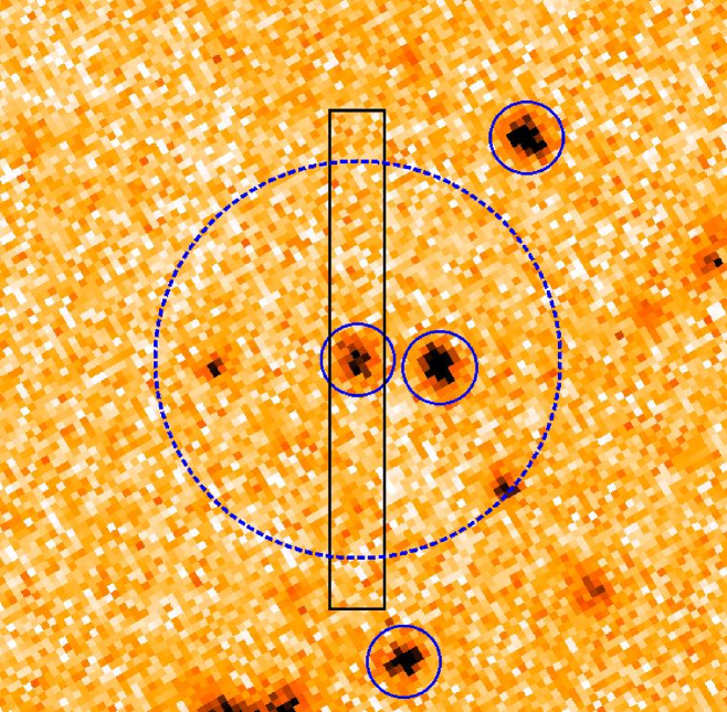
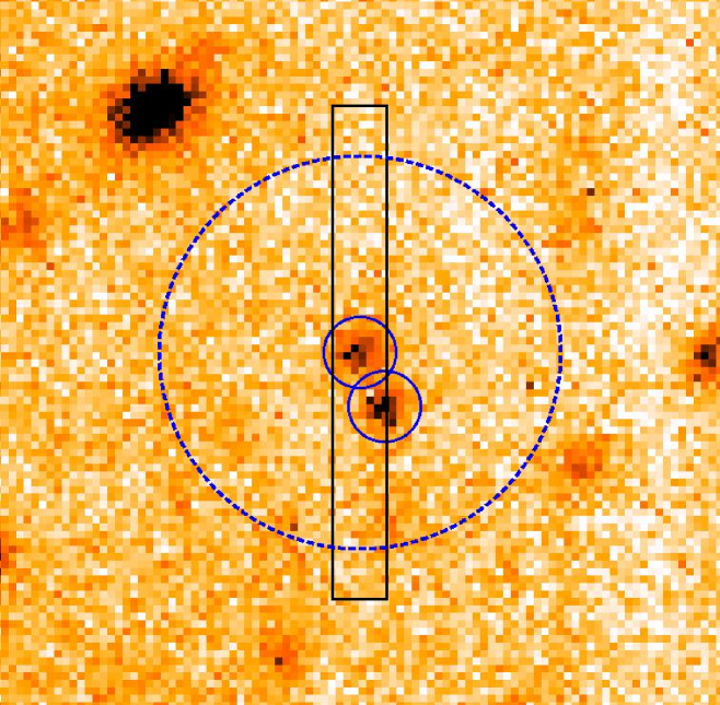
Figure 1: Illustration of conventional spectroscopic slit geometry (data from the survey of Cooke et al. (2005)) and mocked-up in our simulation analysis. In both panels, the geometry of the spectroscopic slitlets is shown by the rectangles, the colour-selected $z\sim 3$ LBGs are marked using small circles, and a radius $30h^{-1}$ kpc at $z=3$ is denoted by a large (dashed) circle centred on the targeted LBG. Although the actual slitlet dimensions vary for each target, those illustrated here have the average dimensions of our survey (see text). The direction of the spectroscopic dispersion precludes acquisition of objects to the left and right of the slitlets as depicted in the two panels. For example in the left panel, the close companion to the immediate right of the targeted galaxy, as well as the more distant companion to the upper right in this highly clustered case, cannot receive spectroscopy and must await future observations which are not always possible. Occasionally, the bulk of the flux of an LBG pair will fall serendipitously into a slitlet as shown in the right panel. Each slitlet in the survey is among $\sim 30-40$ similarly aligned slitlets acquired per telescope pointing that are oriented to minimize atmospheric dispersion at the time of the observations and not designed to align with the orientation of close pairs. As a result, any LBG pairs that fall into the slitlets randomly sample the true underlying close pair fraction.

Figure 2: The cumulative mass function of host haloes as derived from our $120$ $h^{-1}{\rm Mpc}$ simulation box at $z=3$. Error bars estimate cosmic variance using jackknife errors from the eight octants of the computational volume.

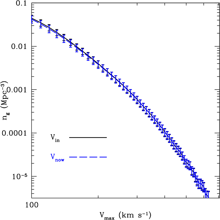
Figure 3: The vertical axis shows the cumulative number density of galaxies in our simulation catalog as a function of velocity using $V_{in}$ (solid black line) and $V_{now}$ (blue dashed line) at $z=3$ to identify subhaloes as galaxies . The error bars shown were generated by summing in quadrature the jackknife error and the realisation-to-realisation scatter and represents errors due to cosmic variance in the simulation.

The color-selection technique ((e.g. Steidel et al., 2003; Cooke et al., 2005) is highly efficient in targeting $z\sim 3$ LBGs and removing background and foreground sources. The observed 2-D color-selected close pair fractions were estimated after a correction for chance alignments by generating random catalogs matched to the density, dimensions, and photometric selection functions specific to the C05 and Steidel et al. (2003) surveyed fields.

2.2 Simulations

The simulation used for the large scale structure and host haloes was performed using the Adaptive Refinement Tree (ART) $N$-body code (Kravtsov et al., 1997) for a universe with a standard cosmology of $\Omega_{m}=1-\Omega_{\Lambda}=0.3$, $h=0.7$, and $\sigma_{8}=0.9$. The simulation followed the evolution of $512^{3}$ particles in a comoving box of $120h^{-1}{\rm Mpc}$ on a side, with a particle mass of $m_{p}\simeq 1.07\times 10^{9}h^{-1}M_{\odot}$. More details can be found in Allgood et al. (2006) and Wechsler et al. (2006). The root computational grid was comprised of $512^{3}$ cells and was adaptively refined according to the evolving local density field to a maximum of $8$ levels. The peak spatial resolution is $h_{\mathrm{peak}}\simeq 1.8~{}h^{-1}{\rm kpc}$ in comoving units.

In this simulation the distinct host haloes are identified using a variation of the Bound Density Maxima algorithm (BDM, Klypin et al., 1999). In this method each halo is associated with a density peak. This peak is identified using the density field smoothed with a $24$-particle SPH kernel (see Kravtsov et al., 2004, for details). The halo virial radii and mass are calculated for the host halo in the simulation box.

The halo virial radius, $R_{\rm vir}$, is defined as the radius of a sphere whose centre is the density peak, with mean density $\Delta_{\rm vir}(z)$ times the mean density of the universe. The virial overdensity $\Delta_{\rm vir}(z)$ comes from the spherical top-hat collapse approximation. In our case this is computed using the fitting function of Bryan & Norman (1998). The simulation assumes a conventional $\Lambda$CDM cosmology which yields $\Delta_{\rm vir}(z=0)\simeq 337$ and $\Delta_{\rm vir}(z)\rightarrow 178$ at $z\lower 2.58334pt\vbox{\hbox{$\buildrel\textstyle>\over{\sim}\ $}}1$. The virial mass is used to characterise the masses of distinct host haloes, the haloes whose centres do not lie within the virial radius of a larger system.

Figure 2 shows the host halo mass at $z=3$ from the procedure described above. The Figure illustrates host halo mass function, complete to virial masses $M\lower 2.58334pt\vbox{\hbox{$\buildrel\textstyle>\over{\sim}\ $}}10^{11.0}h^{-1}M_{\odot}$. The uncertainties are calculated by a jackknife error technique. They are computed by removing one of the eight octants of the simulation volume and recalculating the mass function. These error bars estimate the uncertainty in host halo counts from cosmic variance.

The substructures originally located in these host haloes are removed and replaced by substructures generated using the algorithm of Zentner et al. (2005). This analytic method allows the generation and examination of substructure with effectively unlimited resolution. Each host halo in this simulation catalog has a randomly generated mass accretion history using the extended Press-Schechter formalism (Bond et al., 1991; Lacey & Cole, 1993) with the implementation of Somerville & Kolatt (1999).

Once these mass accretion histories and merger trees are generated, we track the history of the new subhaloes as they evolve. As each subhalo merges into the host it is assigned an initial orbital energy and angular momentum. Then the routine calculates the orbit of the subhalo inside a potential from the host halo between the time of subhalo accretion to the epoch of observation. Tidal mass loss and dynamical friction are modeled to determine the effects of these interactions on the mass of the subhalo. The halo’s density profile is modeled using the the Navarro et al. (1997, NFW) profile with halo concentrations set according to the algorithm of Wechsler et al. (2002). Finally, all subhaloes are tracked until their maximum circular velocities drop below $V_{\rm max}=80$ km s^-1. Haloes which fall below this threshold are removed from the simulation. This step is to avoid excess computing time calculating the small, tightly bound orbits of objects that are not likely to host a luminous galaxy. We refer the interested reader to § 3 of Z05 for the full details of this model.

This process is repeated four times for each host halo to determine the effects of variation in the subhalo populations with a fixed host halo population. In addition to generating substructure catalogs for each separate “realisation” of the model we perform three rotations of each simulation volume. These rotations provide us with different lines of sight through the substructure of the simulation. This provides a total of $12$ effective realisations for us to gather close pair statistics.

Z05 demonstrates that this method is successful at reproducing subhalo count statistics, radial distributions, and two-point clustering statistics measured in high-resolution $N$-body simulations in the regimes we use here. This model’s results agree with numerical treatments over $3$ orders of magnitude, or more, in host halo mass as well as a function of redshift. Moreover, this technique has also proved useful in generating close galaxy pair counts that match observations in the local universe to $z\sim 1$ (Berrier et al., 2006).

In addition to our primary simulation sample described above, a subsample of dark matter haloes from the Millennium-2 simulation (see Boylan-Kolchin et al., 2009, for more details) are used to test our methods in a pure $N$-body simulation.

2.3 Assigning Galaxies to Haloes and Subhaloes

After computing the properties of haloes and subhaloes in a $\Lambda$CDM cosmology, the next step is to map galaxies on to these objects. We use the maximum circular velocity that the subhalo had at the time it was accreted into the host halo, $V_{\rm in}$, to define the objects in our sample. The choice of $V_{\rm in}$ mimics a case where a galaxy is highly resistant to baryonic mass loss when compared to its dark matter halo. As such, the luminosity of the galaxy is unchanged by the loss of matter due to tidal interactions. This case assumes a model in which the luminosity of a galaxy is set in the field and does not change after merging into the host system. Thus we assume that there is a monotonic relationship between halo circular velocity, $V_{\rm max}$, and galaxy luminosity. This model does not account for any effects which might alter the galaxies intrinsic luminosity or which might interfere with observations, such as galaxy-galaxy interactions triggering enhanced star formation or dust obscuration. In effect, this model assumes a perfectly observable universe with a strong halo assumption that galaxy properties are set by the dark matter halos they reside in. The results of Conroy et al. (2006) suggest that this form of SHAM may be used to examine the clustering statistics of $z=2-4$ LBGs. Recent works have suggested that it is reasonable to assume a halo-UV luminosity relation (essentially a halo-star formation rate relation) at the redshifts we examine (Simha et al., 2012; Conroy et al., 2008; Stewart et al., 2009). We discuss the effects of this method of halo assignment on the results in § 3.6.

In addition to the $V_{in}$ model, a second toy model is tested that uses the $V_{max}$ of all haloes at the epoch they are observed. We refer to this model as the $V_{now}$ model. This model describes a physical scenario in which the dark matter and luminous baryonic matter are stripped from subhaloes proportionally. This is in stark contrast to the $V_{in}$ model where the luminous baryons are resistant to mass loss. This second model has proved to be inadequate in reproducing close pairs of galaxies and features observed in the two point correlation function of galaxies locally, but is tested here for the purposes of completeness. Although baryons are likely to be stripped from a halo, it is unlikely that they will be stripped at the same rate as the dark matter. Again, this model does not account for the possibility of enhanced star formation due to galaxy interactions.

Figure 3 shows the cumulative number density of “galaxies” identified in our simulations, $n_{g}$, as a function of their maximum circular velocities. The black solid line shows $z=3$ galaxies using $V_{\rm in}$ as an identifier, while blue dashed line uses $V_{now}$ to generate the function. Our catalogs are complete to a $V_{max}=100$ km s^-1.

In addition to testing a standard SHAM sample and in order to make as direct a comparison as possible with observational data, we match the two-point spatial correlation functions of our model galaxy catalogs to the observed $z\sim 3$ LBG two-point spatial correlation function of Adelberger et al. (2003). The correlation functions are shown in Figure 4. We note that the low-resolution spectra and intrinsic star forming processes of $z\sim 3$ LBGs make it difficult to obtain precise redshifts from the emission and absorption features (Shapley et al., 2003; Adelberger et al., 2003). We consider the effect of LBG redshift uncertainties on the pair fractions in the next section. The spatial correlation functions of Adelberger et al. (2003) used here, incorporate LBG angular information and adopt a prescription (see Appendix C of that work) that aims to minimize redshifts errors in order to estimate the true three-dimensional correlation function. We fit the region from approximately the innner separation radius computed by that prescription out to higher radii and thus heavily dominated by the two halo term region.

The resulting three dimensional two-point correlation function from the simulations is averaged over all four catalogs, with errors including realisation-to-realisation scatter and jack knife errors. Both the fit to the observed “real space” correlation function and the simulation follow a power law of the form:

$$\xi(r)=(r/r_{0})^{-\gamma},$$ (1)

where $r_{0}$ is the spatial correlation length and $\gamma$ is the power law slope. The analysis of C06 places the correlation length at $r_{0}=3.3\pm 0.6$ using a fixed $\gamma=1.6$, whereas the results of Adelberger et al. (2003) find a value of $r_{0}=4.0\pm 0.6$ with $\gamma=1.57\pm 0.14$ for the larger S03 survey dataset. When matching the two-point correlation function of the simulation to the data we find that haloes with $V_{in}\geq 133$ km s^-1 best-fit the parameters of the observations. These haloes produce values of $r_{0}=3.93\pm 0.61$ and $\gamma=1.57\pm 0.05$. The $V_{now}$ model that best matches the observed correlation function is found to have $V_{now}\geq 142$ km s^-1with $r_{0}=3.99\pm 0.64$ and $\gamma=1.54\pm 0.05$.

As discussed above, the spatial distribution, or clustering, has been used to infer the average mass of LBGs in the context of $\Lambda$CDM cosmology. Adelberger et al. (2005) and C06 find the mass of the m${}_{R}\lesssim 25.5$ LBG spectroscopic sample to be $\langle M\rangle\sim 10^{11.6\pm 0.3}M_{\odot}$. The mean mass of our sample compares well at $\langle M\rangle=10^{11.54}h^{-1}M_{\odot}$.

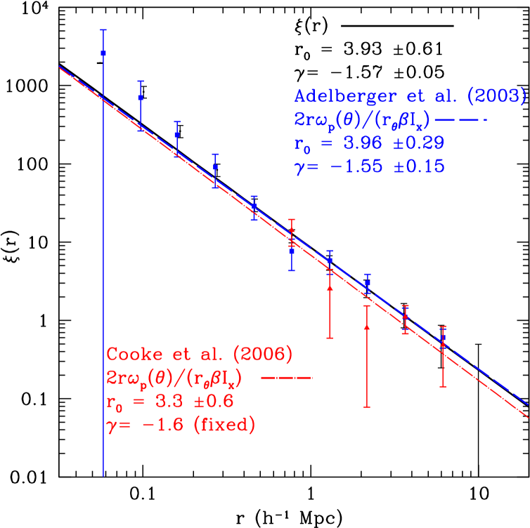
Figure 4: The three dimensional two-point correlation functions. The blue dashed line, and square points, are the real space two point correlation function measured from $z\sim 3$ LBG observations of Adelberger et al. (2003). The red dot-dashed line, and triangular points, are the real space two point correlation function measured from $z\sim 3$ LBG observations Cooke et al. (2006b). Both sets of observations are converted from angular correlation functions to three dimensions using the approximation from Adelberger et al. (2003). Here the $\beta$ and $I_{x}$ are the Beta function and the incomplete Beta function. The solid black line is the spatial two point function generated from the four simulations. The uncertainties are generated by a combination of jack-knife errors and realisation to realisation scatter. Using haloes with $V_{in}\geq 133$ km s^-1 in our simulations results in the best match to the observations.

2.4 Defining Close Galaxy Pairs

Now that we have selected our candidate LBG haloes we must determine the best way to “observe” our sample in order to make direct comparisons with observational results. We examine spectroscopically discernible LBG pairs first.

We define a spectroscopic close pair three ways. Our first criteria include galaxies with a separation of $10-30~{}h^{-1}{\rm kpc}$ on the sky a relative velocity difference in the range of $-500\leq V_{diff}\leq 500$ km s^-1. The separation range on the sky reflects a conventionally determined distance in which close galaxy pairs are considered merger candidates and is designed to exclude close pairs that would likely appear as a single galaxy in the images. The velocity difference, if assumed to be dominated by the peculiar velocities of the galaxies, corresponds to the haloes that have a high probability of merging. The $10-30~{}h^{-1}{\rm kpc}$ separation is well measured by our data. The compact, near point source nature of $z\sim 3$ LBGs and the typical FWHM seeing of the images allows separation of individual galaxies down to $\sim 6h^{-1}$ kpc and the average length of the slitlets used in the spectroscopic observations is $\sim 37.7~{}h^{-1}{\rm kpc}$ at $z=3$, with the bulk of the slitlets probing beyond the conventional maximum separation.

The spectroscopic FWHM resolution of our observations is $\sim 400$ km s^-1 but velocity offsets as small as $\sim 200$ km s^-1 can be measured using multiple cross-correlated spectral lines and high-significance Ly$\alpha$ features. As a result, we test a second criteria that includes pairs with $0-10~{}h^{-1}{\rm kpc}$ separations in projection on the sky for objects that may appear indistinguishable in the images but show clear indications of two separate spectra with a sufficiently large velocity difference ($V_{diff}=\pm 200$ to $\pm 500$ km s^-1).

Finally, we exploit the behaviour of the prominent Ly$\alpha$ feature in $z\sim 3$ LBGs which can be observed in absorption, emission, or a combination of both. The peak of this feature in emission is observed to be redshifted from the systemic redshift by $450\pm 300$ km s^-1(Adelberger et al., 2003), with the tail of the distribution extending beyond $1000$ km s^-1. The observed redshifted peaks are attributed to galactic-scale outflows driven by stellar and supernovae winds. In this picture, the blue wing of the Ly$\alpha$ emission feature is absorbed by neutral gas moving toward the observer and Ly$\alpha$ photons traveling away from the observer are shifted off-resonance as they scatter off receding portions of the outflow, enabling their escape back toward the observer.

C10 find that every LBG in the serendipitous spectroscopic close pairs in their sample and every spectroscopic LBG with a colour-selected close ($\lesssim 20~{}h^{-1}{\rm kpc}$) LBG exhibits Ly$\alpha$ in emission. Because the Ly$\alpha$ feature is typically detected at high significance, we test a third criteria that includes close pairs with no minimum separation on the sky and with no $V_{diff}$. The large velocity dispersion Ly$\alpha$ peaks can help to enable the identification of LBG pairs with little or no actual velocity difference. Random samplings of the Ly$\alpha$ emission velocity offsets show that nearly all such galaxy pairs should be spectroscopically discernible.

To summarise we test three different criteria to select close pairs. Each of these criteria use a maximum outer radius of $30~{}h^{-1}{\rm kpc}$ and a maximum velocity difference of $\pm 500$ km s^-1. The remaining parameters for the different criteria are:

• (A) Pairs with minimum separations less than $10~{}h^{-1}{\rm kpc}$ are always excluded (our fiducial sample for the cylinders). This is designated as $N_{c}$ for cylinders and $N_{cs}(A)$ for spectroscopic slits.

• (B) Pairs with minimum separations between $0-10~{}h^{-1}{\rm kpc}$ are included (thus pairs with separations $0-30h^{-1}$ kpc are considered) if there velocity difference is $V_{diff}\geq 200$. These results are labeled $N_{c}(B)$ for cylinders and $N_{cs}(B)$ for spectroscopic slits. This case allows us to test an intermediate case between criteria (A) and (C).

• (C) No minimum separation or velocity difference. All pairs with separations $<30h^{-1}$ kpc and $-500<V_{diff}<500$ km s^-1 are identified. This will be our fiducial sample for the spectroscopic slit measurements, $N_{cs}$. These are reported as $N_{c}(C)$ for cylinders and $N_{c}$ for spectroscopic slits.

The differences in the results of these three criteria are small (see § 3.1).

With these parameters we calculate the close pair fraction of galaxies. This quantity is defined as:

$$N_{c}\equiv\frac{2n_{\rm p}}{n_{g}}.$$ (2)

Here $n_{\rm p}$ is the number density of pairs and $n_{g}$ is the number density of galaxies in the sample volume. Thus $N_{c}$ reflects the fraction of galaxies that have close companions.

2.5 Spectroscopic Companions

We can perform an analysis of the underlying close pair fraction using the serendipitous spectroscopic LBG pairs of C10 and by mimicking the observation approach of these data in the simulation. In order to best determine the probability of observing a serendipitous spectroscopic pair in the simulation, we generate slits in two specific ways. Firstly, we construct mock slits having the actual lengths and widths used in the observations with the objects placed at the observed locations in the slitlets. We place a randomly assigned slit on the candidate LBG haloes in the simulation and then rotate the slit through $360$ degrees, in steps of $20$, to compute the average $N_{cs}$ for all pairs “observed”. Within the slit geometry we utilise criteria (C) above as our fiducial sample. Measurements made in these randomly assigned slits are designated $N_{cs}(R)$.

Secondly, we recompute $N_{cs}$ from our simulations using a prototypical slit length and width to make a generalized “observation”. The prototypical slit has a width of $1.37$ arcsec, the mean width of the slits used in the observations, for a half width of $3.7~{}h^{-1}{\rm kpc}$. The prototypical slit length is $60.0~{}h^{-1}{\rm kpc}$, which is $11.13$ arcsec at $z=3$. All lengths are given in proper, physical units. The $N_{cs}$ measured in the spectroscopic slit only incorporates pairs observed in one of the rotations of the slit. Thus the $N_{cs}$ is smaller then the total $N_{c}$ for any of the criteria discussed above. Because the candidate LBG haloes are centred in the prototypical slits we only need to perform $10$ rotations over $180$ degrees to determine the random slit count. Again, we use criteria (C) above as our fiducial sample. Modeling the observations in these two ways enables a direct comparison to the C10 analysis and provides results that can be applied in a more general way to any conventionally acquired survey.

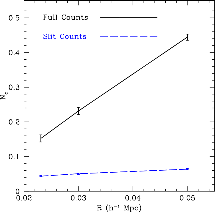
Figure 5: The dependence of the close pair fraction on the maximum separation between the central galaxy and its companion. All data is calculated at $z=3$. The solid black line is the full cylinder sample. The blue dashed line is the close pair fraction for the spectroscopic slit sample. Uncertainties are calculated from a combination of the standard deviations of the four realisations and jack knife errors in the individual simulation boxes.

We may also characterise the dependence of the sample on the maximum pair separation used. As observed in Figure 5, increasing the maximum radius used for our close pair counts increases our resulting $N_{c}$. Though the increase is comparatively small in the spectroscopic slit, we can see in Figure 5 that it is significant for the full cylinder sample.

2.6 Photometric Companions

We make one other measurement in this work. We examine the apparent angular, or “photometric”, close pair fraction, $N_{p}$, and it’s impurity. A photometric close pair is defined as one in which we have no cut on velocity, and also no pairs are allowed within the minimum radius. This is essentially a single line of sight through the box designed to mimic the companion counts observed in the plane of the sky in photometric surveys that utilise simple LBG colour selection criteria at $z\sim 3$.

Our simulation identifies close pairs within a redshift range of $\delta z\sim 0.18$ at $z=3$. The criteria of S03 and C05 select LBG populations with $\langle z\rangle=3.0,1\sigma=0.3$. While our simulation samples $\sim 25$ per cent of the LBGs detectable in $z\sim 3$ surveys, it probes a large enough redshift path to distinguish objects that are, and are not, physically clustered. This is true in part because clustering effects are negligible beyond a radius of $\sim 10h^{-1}{\rm Mpc}$. Thus we can use our analysis to provide an estimate of $N_{c}$ and the sample impurity. Our results for this work are found in section 3.2.

2.7 Diagnosing the effects of Interlopers

Our method characterises the probability of chance projections being identified as a companion galaxy. We define the sample impurity as the fraction of ”observed” close pairs in the simulation, using the criteria described above, that do not reside inside a mutual dark matter halo and are not a physically interacting pair. The total sample impurity is given by

$$I\equiv\frac{n_{\rm f}}{n_{c}}.$$ (3)

Here $n_{\rm f}$ is the number density of false galaxy pairs in the sample volume and $n{\rm{}_{c}}$ is the number density of galaxy pairs observed in the sample.

Figure 6 identifies the sample impurity as it evolves with the radii of the cylinder used. In this case we see how impurity is effected by the maximum size of the cylinder. This is of course a simple relationship. As we increase our maximum radius we have a greater chance of identifying a pair of companion galaxies, but also a greater risk of picking up a chance projection of two physically unassociated galaxies. In this figure the uncertainties are calculated by summing in quadrature an error associated with cosmic variance, calculated by a jack knife error method, and a realisation-to-realisation scatter.

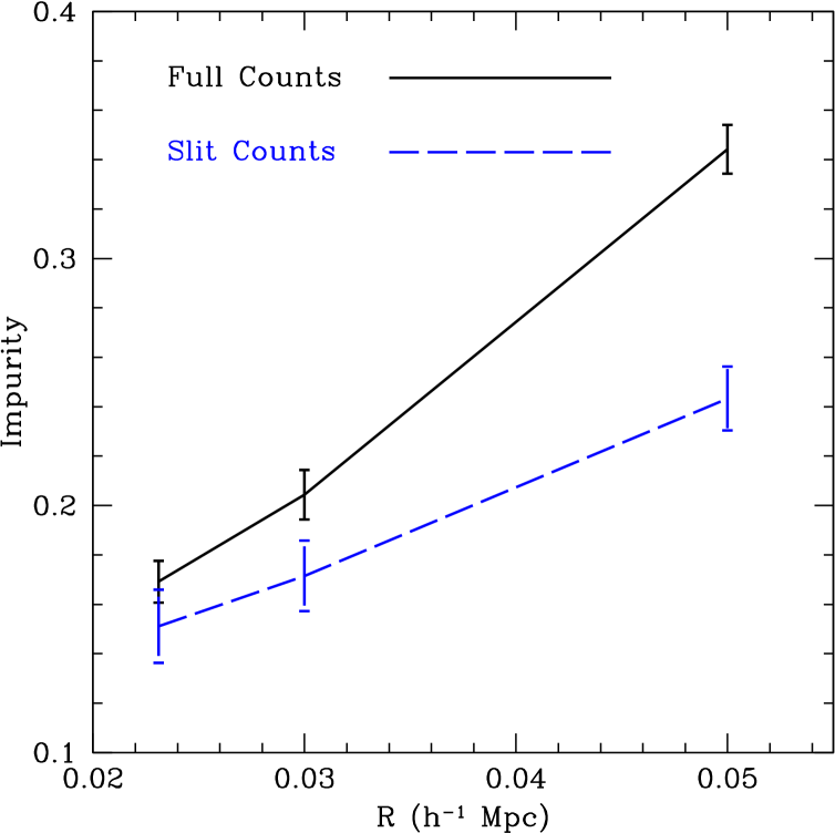
Figure 6: The measured sample impurity using a varying outer radius. The solid black line shows the impurity fraction for the full cylinder sample, while the blue dashed line shows the impurity for the randomly oriented spectroscopic slit sample. Uncertainties are calculated from a combination of the standard deviations of the realisations and jack knife errors in the individual simulation boxes.

We also examine the effect that extending the maximum velocity between galaxies has on both the pair fraction and the sample purity. Figure 7 shows this relationship. As before, using a larger velocity cut increases both our pair fraction and sample impurity. The error bars are calculated in the same manner as Figure 6.

In the observational samples of S03 and C05, the color-selection techniques are highly efficient ($\gtrsim$90% effective) in targeting $z\sim 3$ LBGs and removing background and foreground sources as determined by the spectra. The observed 2-D color-selected close pair fractions reported below were corrected for impurity by generating random catalogs matched to the density, dimensions, and photometric selection functions specific to the C05 and S03 surveyed fields and computing the fraction of random unassociated pairs occurring within the projected separations for the criteria described above.

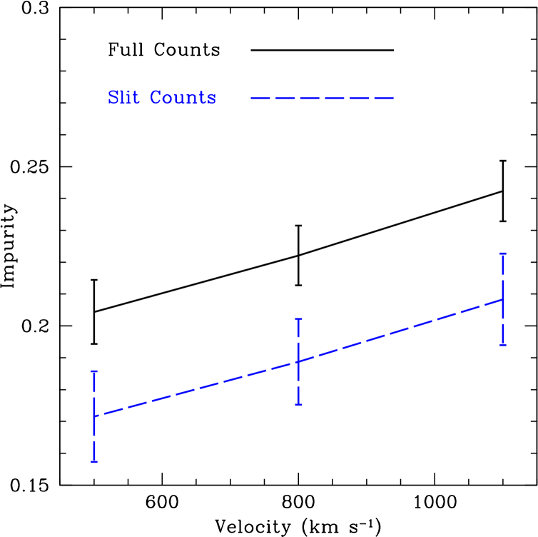
Figure 7: The measured sample impurity using various velocity cuts. The solid black line indicates the impurity of the sample for the full cylinder counts. The dashed blue line is the impurity recorded for the randomly oriented spectroscopic slit sample. Uncertainties are calculated from a combination of the standard deviations of the four realisations and jack knife errors in the individual simulation boxes. Interestingly this demonstrates that large maximum velocities do not significantly increase sample impurity over the range shown here.

2.8 Galaxy Number Density Problem

For our $z=3$ comparisons we adopted a sample of potential LBGs that best describes the data and has $V_{in}\geq 133$ km s^-1, that is, the $V_{max}$ of a subhalo when it is initially accreted into a host, or simply the $V_{max}$ of the object if the halo is an independent host halo. In addition to matching the two point correlation function, these models produce a comoving number density of galaxies, $n_{g}$, that may also be compared to the observational sample. The volumetric comoving number densities for the two models are $n_{g}(V_{in}\geq 133$ km s${}^{-1})=0.019\pm 0.003$ h³ Mpc^-3 and $n_{g}(V_{now}\geq 142$ km s${}^{-1})=0.01442\pm 0.00003$ h³ Mpc^-3.

The comoving number densities for more massive haloes are: $n_{g}(V_{in}\geq 200$ km s${}^{-1})=0.0039\pm 0.0006$, h³ Mpc^-3 and $n_{g}(V_{in}\geq 300$ km s${}^{-1})=0.00059\pm 0.00010$ h³ Mpc^-3 . While we see that the $V_{in}\geq 200$ sample has a better match to the number density of $\sim 0.004\pm 0.002$ h³ Mpc^-3 from LBG observations (see below for further details), this sample does not match the observed correlation function and produces a significantly lower value for $N_{c}$.

The matched $V_{now}$ sample has a surface density in comoving coordinates of $6.14$ h² Mpc^-2, $10.2$ galaxies arcminute ^-2, compared to $8.2$ h² Mpc^-2, $13.6$ galaxies arcminute ^-2 for the $V_{in}$ sample. Both of these values exceed the $\sim 1.7$ galaxies arcminute ^-2 from observation. These surface densities are measured from the length of the $120h^{-1}{\rm Mpc}$ box at $z=3$, a redshift range of $\delta z\sim 0.2$ and then corrected for the total redshift pathlength observed in the surveys and the efficiency of LBG detection as a function of redshift from the colour selection (assumed to be $100$ per cent efficient near $z=3$, e.g., no lost galaxies as a result of bright stars, low S/N regions on the chip, colour detection efficiency, etc., as is the case for the observations).

Previous research has uncovered similar discrepancies between the number density of matched massive haloes and that observed for $z\sim 3$ LBGs using different types of simulations (e.g., Davé et al., 2000; Ouchi et al., 2004; Nagamine et al., 2005; Lacey et al., 2011). Nevertheless, each propose that the excess $n_{g}$ can be resolved by including other types of high redshift objects, such as dust obscured and/or low star formation rate galaxies and damped Ly$\alpha$ absorption systems (DLAs). The model of Lacey et al. (2011) suggest that without dust extinction the number of LBGs would be $\sim 5$ times the number observed. This model also recreates the properties of the observed sample once dust extinction is included. Thus, we report our results using the full (high-density) sample below and explore the effects of the density mismatch on the results in section 3.4.

3 Results

Using the methods described in Section 2.3 we calculate: ($1$) the close pair fraction observed serendipitously in the spectroscopic slits, $N_{cs}$, ($2$) the $10-30~{}h^{-1}{\rm kpc}$ total spectroscopic close pair fraction, $N_{c}$, ($3$) the $10-30~{}h^{-1}{\rm kpc}$ photometric close pair fraction, $N_{p}$.

As a reminder, all three sample criteria include pairs with separations $<30$ $h^{-1}$kpc and a velocity difference of $\pm 500$ km s^-1. However, the differences are that criteria (A) excludes all pairs with separations $<10$ $h^{-1}$kpc , criteria (B) includes pairs with separations $<10$ $h^{-1}$kpc if their velocity difference is $>200$ km s^-1, and criteria (C) includes pairs with separations of $<10$ $h^{-1}$kpc with no restriction on the velocity difference.

3.1 Spectroscopic Close Companion Counts at z=3

We first note that the observations of C10, to which we are comparing these results, find a serendipitous close pair fraction of $N_{cs}=0.071\pm 0.023$ in the spectroscopic slits for the highest confidence subsample ($140$ LBGs) and $N_{cs}=0.047\pm 0.015$ for the full sample of $211$ LBGs. In our simulations we “observe” serendipitous close pairs using the three different sets of criteria discussed in § 2.4.

In our randomly selected slit length sample (lengths and object positions matched to the survey of C05) we find $N_{cs}(R)(A)=0.0220\pm 0.0234$, $N_{cs}(R)(B)=0.0300\pm 0.0178$, and $N_{cs}(R)(C)=0.0430\pm 0.0145$. All three results are consistent within their uncertainties.

For the prototypical slit length of $60.0~{}h^{-1}{\rm kpc}$, we find an “observed” $N_{cs}(A)=0.0293\pm 0.0013$, $N_{cs}(B)=0.0375\pm 0.0016$, and $N_{cs}(C)=0.0506\pm 0.0017$.

As before, the uncertainties are a combination of jack knife errors from cosmic variance and realisation-to-realisation scatter. These measurements reflect our uncorrected sample and include galaxies that meet our velocity criteria and are observed as close pairs due to projection effects even though they do not reside in the same parent halo.

Finally, the full observable pair fraction in the cylinder is $N_{c}(A)=0.228\pm 0.006$, $N_{c}(B)=0.246\pm 0.006$, and $N_{C}(C)=0.275\pm 0.007$. As expected, criteria (B) and (C) produce slightly higher values, but they are not significantly different from our fiducial value (A).

We report the results of criteria (A) for the cylinder and criteria (C) for the spectroscopic slits because criteria (A) is designed to match the morphological and close pair fraction analyses in the literature and criteria (C) is best matched to the methodology of the spectroscopic slit analysis of C10.

Close pair fraction predictions for the full uncorrected observable $N_{c}$ and the spectroscopic slit may be found in Figure 8. Note that these values are not corrected for line of sight projection effects. Here we track objects in the catalog from $0\leq z\leq 3$ that have a number density matched to a $z=3$ sample with $V_{max}$ greater than four different critical values. By holding a constant $n_{g}$ cut we examine the changes in $N_{c}$ at a fixed population size with redshift. The solid black curve represents the close pair fraction for a galaxy sample with $V_{in}\geq 133$ km s^-1 utilising our standard criteria (A). The green dodecagonal point and the magenta dash point (offset to $z=2.9$ and $z=3.1$ for clarity) are the observed serendipitous close pair values of the highest confidence and total $z=3$ sample, respectively. The solid black triangle denotes the results from our fiducial slit criteria (C) and is consistent with both observational samples.

The blue dashed line and the red dot-dashed line represent more stringent mass cuts with values of $V_{in}\geq 200$ km s^-1 and $V_{in}\geq 300$ km s^-1, respectively, using the standard cylinder. These values are included to make a comparison of $N_{c}$ with $n_{g}$, the (comoving) number density of galaxies, as has been done in work by other authors, even though their correlation functions do not closely match the observations. In these cases we may examine the evolution of higher mass subsamples with a fixed $V_{in}$, with redshift. The solid blue square and the solid red hexagon represent the expected slit model $N_{cs}$ for these higher mass cuts. As we can see, they are both well below the expected $N_{cs}$ from the LBG observations.

The light blue short-long dashed line and the light blue triangle represent the value for our $V_{now}\geq 142$ sample. This model also underpredicts $N_{c}$, and does so even when matched to the number density of galaxies, $n_{g}$, at all redshifts (see Berrier et al. (2006) for more detail). As this model demonstrates the same flaws as our $V_{in}$ model and does not reproduce the observed $N_{c}$ down to low-$z$, it will be excluded from further discussion.

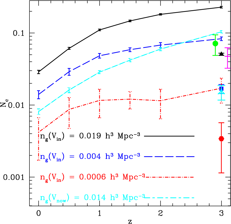
Figure 8: Expected spectroscopic close pair fractions. Plotted are the expectations from $z=0-3$ for different number densities of galaxies corresponding to the specified velocity cuts at $z=3$. The results report the pair fraction in cylinders with radii $r<30~{}h^{-1}{\rm kpc}$ (curves). The expected $N_{cs}$ at $z=3$ for the serendipitous pairs in ”observed” spectroscopic slits are also plotted (points). The solid black curve and triangle point represent the close pair fraction of galaxies, $N_{c}$, in our fiducial sample of haloes using the $V_{in}\geq 133$ km s^-1 cut at $z=3$, and the same number density at all previous redshifts, matched to the LBG correlation function observations. Similarly, the light blue short-dash long-dashed curve and empty triangular point represent our fiducial $V_{now}\geq 142$ km s^-1 sample at $z=3$. More massive and brighter samples are shown with number densities matching the values of $V_{in}\geq 200$ km s^-1 (blue dashed curve, square point) and $V_{in}\geq 300$ km s^-1 (red dot-dashed curve, hexagonal point) at $z=3$. Uncertainties shown for the randomly oriented slits are calculated from a combination of jack knife errors and variance between the four realisations used. Please note that these points are not corrected for sample impurity due to projection effects. The green dodecagonal point at $z=2.9$ and the magenta dash point at $z=3.1$ represent the observed $N_{c}$ from the high signal to noise sample and the full observed sample of $z\sim 3$ LBGs (Cooke et al., 2010), respectively, and are offset from $z=3$ for clarity.

At our fiducial slit radius of $30.0~{}h^{-1}{\rm kpc}$ the sample impurity is $I=0.1716\pm 0.0111$ for the slit and $I=0.2225\pm 0.0099$ for the full cylinder count. These values imply that we have $(1-I)$ $N_{c}$, or a real $N_{cs}\sim 0.042\pm 0.0015$ (cf. $N_{cs}=0.0506\pm 0.0017$, uncorrected) in the slits and $N_{c}\sim 0.177\pm 0.005$ (cf. $N_{c}=0.228\pm 0.006$, uncorrected) for the full cylinder.

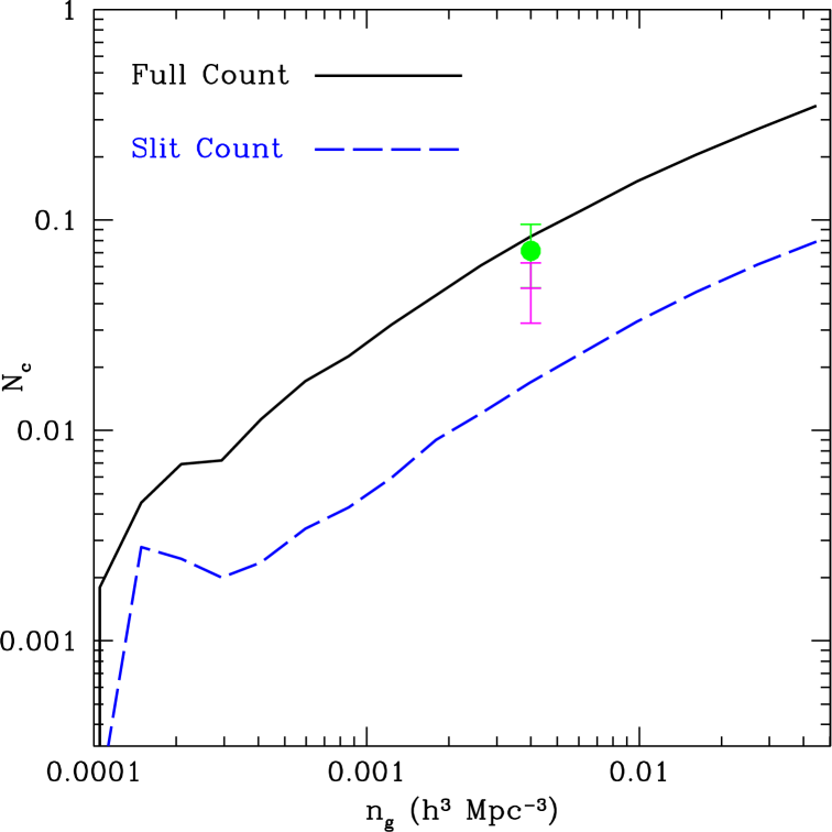
Figure 9: Variation of the $z=3$ close companion count ($N_{c}$) with galaxy number density ($n_{g}$). The black solid line gives the $N_{c}$ for the full cylinder while the blue dashed line gives the $N_{cs}$ for the randomly oriented spectroscopic slits. The green octagonal point represents the observed serendipitous close pair fraction for the high confidence sample in the spectroscopic slits, at the observed number density, in the sample of Cooke et al. (2010). The magenta hash is the pair fraction for the total observed sample.

We can generalize the results of Figure 8 to Figure 9. We examine the values of $N_{c}$ in both the spectroscopic slit (blue dashed curve) and the full cylinder with radius $10\leq r\leq 30$ h^-1 kpc (black solid curve) as a function of the number density of “galaxies” in the sample, $n_{g}$. Here, the observational spectroscopic slit results seems too high for the observed LBG number density ($n_{g}\sim 0.004\pm 0.002$ h³ Mpc^-3) and appears to be more consistent with pair fraction at the density of our full $V_{in}\geq 133$ km s^-1 sample which is $\sim 5\times$ higher. What causes this inconsistency? We discuss this issue in $\S$ 3.4

3.2 Angular Close Pair Fraction

We also use our simulation to estimate the observed angular, or “photometric”, close pair fraction, $N_{p}$. In this case, we calculate a pair fraction without using a velocity cut and exclude all objects inside the minimum projected radius of $10h^{-1}$ kpc. As discussed above, it is possible to approximate the $N_{p}$ at $z=3$ in the simulation box. The simulation is $120h^{-1}{\rm Mpc}$ long in the comoving coordinates, and thus at $z=3$ has an approximate redshift length of $\delta z=0.18$ from front to back. Due to clustering effects being less pronounced beyond $10h^{-1}{\rm Mpc}$ we may use this box for this purpose, despite the redshift range for the survey being $\delta z\sim 0.6$. Thus, while we can easily determine $N_{p}$, we must be cautious that this is only an approximate value.

Figure 7 provides us with some estimate of the effects of a larger velocity cylinder on the purity of the sample. In the case of our photometric sample we are using an equivalent velocity difference based on the total length of the box in local Hubble flow as well as the peculiar velocities along the line of sight for the galaxies. Similarly we can see from Figure 6 that the sample’s impurity increases with larger sample radius. In the case of $30~{}h^{-1}{\rm kpc}$ this is $\sim 0.20\pm 0.01$ from the on the sky dimension of the cylinder alone.

We examine this solely at $z=3$ in a fashion similar to Figure 9 for our photometric pairs sample. The result is Figure 10, which presents $N_{p}$ as a function of $n_{g}$. The solid black line is the observed $N_{p}$, and the blue dashed line is the fraction of galaxies that are actually physically associated.

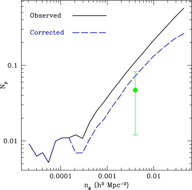
Figure 10: The photometric close pair fraction at $z=3$ as a function of the number density of galaxies in the sample. The solid black line is the observed photometric close pair fraction. The blue dashed line is the close pair fraction for the physically associated sample only. This line illustrates only the fraction of galaxies that would be mutually inside the same hosting dark matter halo. The green octagonal point represents the observed close pair fraction for a sample of photometrically observed LBGs from Cooke et al. (2010) (see text for further details).

We find a photometric close pair fraction, $N_{p}$, of $0.336\pm 0.009$ before correcting for impurity. After this correction we find $N_{p}\sim 0.189$, which agrees with our predicted $N_{c}$. The discrepancy between the “observed” and the physically associated fraction, the “pure” portion of the sample without line of sight contaminants, is reasonable due to the large effective length of the cylinder used in these measurements. The corrected fraction reflects the “real” close ($<30~{}h^{-1}{\rm kpc}$) companion count and therefore the real fraction of interacting galaxies.

These results are interesting when compared with the results presented in Conselice et al. (2003), Bertone & Conselice (2009), and Bluck et al. (2009) which produce similar statistics for these high redshift objects. The close pair fractions we find are consistent with the merger fractions estimated in these works for other observed large samples of galaxies using close galaxy pairs as well as estimates based on the concentration-asymmetry-clumpiness (CAS) method. Conselice et al. (2003) estimates an apparent merger fractions of bright LBG’s at $z\geq 2.5$ to be between $40-50$ per cent. Bluck et al. (2009) identifies $82$ massive galaxies, $M_{*}>10^{11.0}M_{\odot}$ in a redshift range of $1.7-3.0$. These are further divided into a sample of 44 galaxies between $1.7<z<2.3$ and $38$ galaxies from $2.3<z<3.0$. Close pair fractions are estimated for the two samples by identifying all imaged galaxies within $\pm 1.5$ magnitudes of the sample galaxies magnitude that reside within an $R_{max}<30$ kpc (physical, $h=0.7$) and statistically corrected for impurities. Please note that only the original $82$ galaxies have redshift information, the rest of the galaxies included in the measurement are photometric pairs. The observed $N_{p}$ for the $1.7<z<2.3$ ($2.3<z<3.0$) are $N_{p}=0.19\pm 0.07$ ($N_{p}=0.40\pm 0.10$). These observed high redshift values are consistent with our estimates in both the corrected and uncorrected sample. Bertone & Conselice (2009) examines models of galaxy merger rates comparing simulations and observational results. This work also finds a high merger rate at high redshift.

3.3 Comparison To Previous Results

In order to demonstrate the usefulness of this technique in calculating $N_{c}$ across a wide range of redshifts we make a comparison to several previous existing measurements at low redshift (see Berrier et al. (2006) for further discussion on these samples). The samples used in this comparison are extracted from the SSRS2, CNOC2, and the DEEP2 surveys Patton et al. (2002); Lin et al. (2004). These surveys provide several candidate definitions for a close pair. To match the technique used in the observations we use criteria (A). In order to determine the sample of haloes used in our simulation, both host dark matter haloes and substructure, we match the number density of galaxies from the observations to the number density of haloes in the simulation using the $V_{in}$ model as in Berrier et al. (2006).

To extend this method to $z\sim 3$, we examine observed colour-selected LBG pairs with $10-30h^{-1}$ kpc separations from our LBG survey and the larger survey of S03 and find an observed photometric pair fraction of $N_{p}=0.047\pm 0.035$. This result is corrected for spatial impurities that are estimated in a manner similar to that for the low-z samples. We estimate the impurity using mock catalogs constructed to the exact field dimensions and number densities of each observed field. We then distribute mock galaxies using redshift distributions and interloper fractions determined by the photometric selection function. The number of close pairs observed in projection is then corrected to align with the fraction that is found to consist of true pairs in three dimensions.

We then calculate the $z=3$ data in the simulation in the same manner as the low-redshift data and matched it to the LBG number density. From our definition of the close pair fraction, a decrease in number density corresponds to a similar decrease in the close pair fraction. If LBGs randomly comprise $\sim 1/5$ the number of massive haloes as the number densities imply, and thus approximately $1/25$ of our sample would be composed of LBG-LBG pairs, we would expect a lower limit of $N_{c}\sim 0.228\times(1/5)$, or $\sim 0.0456$ ($N_{c}\sim 0.177\times(1/5)$, or $\sim 0.0373$ for the purity corrected sample) for the observed LBG-LBG pair fraction. Our simulated value is still larger than this at $N_{c}=0.083\pm 0.005$ ($N_{c}\sim 0.065$ with purity corrections). For comparison, we look at $N_{p}$ for our photometric pair value after corrections for impurity, as this is the only estimate of the full $N_{c}$ available. This assumes that all galaxies in the fiducial simulation sample which are within the same host halo will be observed, irregardless of the $n_{g}$ issues discussed in § 2.8.

The results of this comparison are presented in Figure 11. Here the solid black line, black points, and solid square points represent the pair fractions calculated from our $n_{g}$ matched samples from $z=0$ to $z\sim 3$. The empty squares are observed values from the DEEP2 Survey taken from fields 1 and 4, Lin et al. (2004) and the triangles are from the CNOC2 and SSRS2 surveys, Patton et al. (2002). The value of $N_{c}$ from the $z\sim 3$ observations is indicated by the green dodecagonal point at $z=3$. The full fiducial sample $N_{c}$ for $z=3$ is shown connected by the dashed line. The $N_{c}$ values determined from the simulations are closely comparable to the matched-density observations in nearby redshift bins across all redshifts observed. The technique used here is more completely described in Berrier et al. (2006).

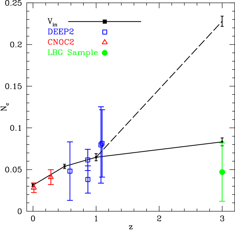
Figure 11: Comparison of $N_{c}$ from $z=0$ to $z=3$ in the simulation with measurements from surveys. The black points, solid squares, and solid line represent the $N_{c}$ calculated from our $n_{g}$ matched samples from $z=0$ to $z=3$. The dashed black line represents $N_{c}$ for our fiducial sample at $z=3$. The empty blue squares are data points from the DEEP2 Survey taken from fields 1 and 4, (Lin et al., 2004). The hollow red triangles are data from CNOC2 and SSRS2, (Patton et al., 2002). The green dodecagonal point at $z=3$ is the $N_{p}$ measured from the LBG surveys of Cooke et al. (2005) and Steidel et al. (2003).

3.4 Galaxy Number Density Problem Revisited

We have matched the 3-D two-point correlation function to produce our fiducial sample of high redshift galaxies. We find that if LBGs comprise all massive haloes in the matched simulation sample, this produces a number density that is too high by a factor of $\sim 4.75$ when compared with the observed LBG number density, as has been similarly found by other authors. In addition, this sample produces a value of $N_{p}$ and $N_{c}$ in the cylinders that is too high by a similar factor but a value of $N_{cs}$ in the spectroscopic slits (that are biased to detecting pairs with separations of $<\sim 20$ h^-1 kpc because of their geometry) that is consistent within the errors of the observations.

In contrast, forcing the sample to match the observed LBG number density yields an $N_{p}$ and cylinder $N_{c}$ similar to the observations but an $N_{cs}$ that is significantly lower than that observed in the slits. Moreover, such a sample ($V_{in}\gtrsim 200$ km s^-1) results in a poor fit to the observed LBG correlation function and corresponds to haloes too massive to be reconciled with the mass of LBGs from clustering analysis.

LBGs do not comprise all massive galaxies at $z\sim 3$. Other identified populations include sub-mm galaxies, passive and star forming BzK galaxies, DRGs, and other galaxy types with typically lower UV luminosities then LBGs. If LBGs represent $\sim 1/4.75$ of the matched massive haloes in our $z\sim 3$ sample, then the agreement in number density produces an $N_{p}$ and cylinder $N_{c}$ that are in very good agreement with the observations but an $N_{cs}$ in the slits that is significantly lower than the observations. In this case, the sample still matches the LBG correlation function (as they are pulled from the same parent population) and thus corresponds to haloes with the same mass as the observations.

Dust obscured galaxies may make up a fraction of the ”missing” massive haloes, however, infrared and sub-mm surveys recover only a small fraction of the number necessary to reconcile the difference. The latter interpretation more accurately reflects the observed LBG population and leaves only the $\lesssim 20h^{-1}$ kpc physical pair fraction in disagreement. The small-scale behaviour (one-halo term regime) measured in accurate 2-D correlation functions that utilise deep, wide-field imaging helps provide the solution to the remaining disagreement and offers interesting insight into the nature and detectability of LBGs.

3.5 Small-scale behaviour: The one-halo term

Measurements of the angular (2-D) correlation function (ACF) at $z\sim 4$ in the Subaru/XMM-Newton Deep Field over $1$ deg^-2 (Ouchi et al., 2005) and at $z\sim 3$ in the Canada-France-Hawaii Telescope Legacy Survey $4$ square-degree Deep fields (Cooke et al., 2012) are able to utilise a large number ($\sim$$10^{4}-10^{5}$) of LBGs to accurately probe the ACF down to $m_{R}\sim 27$ from relatively small to large scales ($\sim 0.5-10~{}h^{-1}$ Mpc, comoving). Both efforts witness a distinct break in the form of the ACF at small scales from the power law fit over larger scales that may provide insight into the discrepancy in the observed and expected close pair fractions in the spectroscopic slits.

In order to measure the angular correlation function at $z=3$ in the simulation, we will follow the method used in previous works such as Conroy et al. (2006) and utilize the Limber transformation.

$$\omega(\theta)=\frac{\int_{0}^{\infty}dzN^{2}(z)\frac{dr}{dz}\int_{\infty}^{\infty}dx\xi(\sqrt{(}r^{2}\theta^{2}+x^{2}))}{[\int_{0}^{\infty}dzN(z)]^{2}},$$ (4)

where $r$ is the comoving distance at $z$ and $N(z)$ is the normalized redshift distribution of the galaxies in the observed sample.

Figure 12 presents the ACFs of our simulation samples and the two observational datasets. As demonstrated in Figure 12, the form of the fiducial ($V_{in}>133$ km s^-1) and observational ACFs in the outer regions are consistent. However, the inner regions show a marked discrepancy. Regardless of the number density, the standard technique of halo assignment cannot reproduce the features of the LBG angular correlation function on both large and small scales. In addition, the mismatch cannot be corrected by any scaling of the data via an integral constraint. Our standard abundance matching model is unable to reproduce the observed break from power law behaviour near $150-200$ h^-1 kpc in comoving coordinates to match both the one-halo and two-halo components of the correlation function to the accuracy of the data without incorporating assumptions of the form of the Limber equation in the inner region.

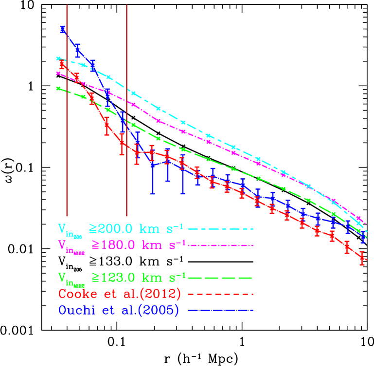
Figure 12: The angular correlation function for samples of dark matter haloes pulled from our primary sample. Two subsamples are taken from the dark matter halo catalog using different $V_{in}$ cuts and are compared with two observational sets. The solid black line is our fiducial sample which matches the three dimensional correlation function of Adelberger et al. (2005). The green long-dashed line is our best match to data from the Millennium-2 simulation sample with $V_{in}\geq 123$ km s^-1. The magenta dot-short dashed line and cyan short-long dashed line represent abundance matched samples with $V_{in}\geq 180$ km s^-1 from Millennium-2 and $V_{in}\geq 200$ km s^-1 from the Z05 simulations respectively. The red short dashed sample represents the observed angular correlation function for $z\sim 3$ from Cooke et al. (2012), and the blue dot-long dashed line illustrates a sample of LBGs at $z=4$ from Ouchi et al. (2005). Both observational samples demonstrate a strong break from a single power law around $100$ h^-1 kpc. None of the simulation samples are able to reproduce this feature through our standard abundance matching techniques. The two dark red solid vertical lines represent the range, in comoving coordinates, that we identify galaxy-galaxy pairs.

If we follow a standard subhalo abundance matching scheme we observe a $N_{c}$ in the cylinder and $N_{p}$ from our mock photometric sample which are consistent with the observed pair counts, however, we do not produce the correct $N_{cs}$ for the mock spectroscopic slits (pairs at $\lesssim 80~{}h^{-1}{\rm kpc}$ in comoving coordinates, or $\lesssim 20~{}h^{-1}{\rm kpc}$ in physical coordinates). $N_{c}$ is smaller than the observed fraction by a factor consistent with the decrease in amplitude of the one-halo term in the correlation function over the same separations.

To further test this result, we analyse the Millennium 2 simulation (Boylan-Kolchin et al., 2009). The Millennium-2 simulation has five times the spatial resolution of the original Millennium simulation, in this case a Plummer equivalent softening of $1~{}h^{-1}{\rm kpc}$. This resolution is more than adequate for our needs. The sample we select from Millennium-2 is well above the resolution limits of the simulation, and thus provide a further test that our results are not adversely effected by resolution issues. Using this simulation, we find the closest match to the two point correlation function of the observations to be a cut of $V_{in}\geq 123$ km s^-1. Haloes with this criterion show a good agreement to the data, with a power law fit of $r_{0}=3.98\pm 1.44$ Mpc h^-1 and $\gamma=-1.47\pm 0.27$. In addition, this sample has a number density $n_{g}=0.017$ h³ Mpc^-3, approximately $4.25$ times larger than the observed $n_{g}$ of LBGs and similar to the overdensity of our primary simulation sample. We have included the Millennium-2 ACFs for the abundance matched sample and for the 3-D correlation function matched sample in Figure 12. Again, the simple abundance matching techniques are not capable of reproducing the shape of the angular correlation function.

This selected sample produces a $N_{c}=0.1521\pm 0.0006$ for our fiducial criteria (A) in the cylinder, and $N_{cs}=0.033\pm 0.001$ for our fiducial criteria (C) in the slits. The sample shows an impurity of $0.1433\pm 0.0176$ in the cylinder and $0.1167\pm 0.0202$ for the slit, thus our corrected values are $0.1303\pm 0.0059$ and $0.02919\pm 0.0014$ for the full cylinder and the spectroscopic slit respectively. For our line of sight mock photometric sample we find $N_{p}=0.2299\pm 0.0144$, before corrections for impurity and $0.1370\pm 0.0154$ after.

To match the number density of observed LBGs we would select a sample of haloes with $V_{in}\geq 180$ km s^-1. As with the previous number density matched sample this has a power law fit of $r_{0}=5.17\pm 2.24$ and $\gamma=-1.56\pm 0.30$. This sample produces a close companion count of only $N_{cs}=0.0101\pm 0.0023$ in the spectroscopic slit, $N_{cs}=0.0089\pm 0.0022$ after impurity corrections, $N_{c}=0.0505\pm 0.0060$ for the full cylinder, only $0.0442\pm 0.0061$ after being corrected for impurity, and $N_{p}=0.0682\pm 0.0092$ photometrically, $0.0471\pm 0.0075$ after correcting for sample impurity.

All results for our primary samples in the Z05 simulations and in Millennium-2 from here and from § 3.1, § 3.2 are summarised in Table 1

Table 1: $N_{c}$ and $N_{p}$ for all samples

Simulation & Criteria	$N_{c}$	Corrected $N_{c}$	$N_{cs}$	Corrected $N_{cs}$	$n_{g}$
Z05 (A)	$0.228\pm 0.006$	$0.177\pm 0.005$	$0.0293\pm 0.0013$	$0.0233\pm 0.0011$	$0.019$
Z05 (B)	$0.246\pm 0.006$	$0.193\pm 0.005$	$0.0375\pm 0.0016$	$0.0305\pm 0.0014$	$0.019$
Z05 (C)	$0.275\pm 0.007$	$0.218\pm 0.006$	$0.0506\pm 0.0017$	$0.0419\pm 0.0015$	$0.019$
Z05(R)(A)	N/A	N/A	$0.0220\pm 0.0234$	N/A	$0.019$
Z05(R)(B)	N/A	N/A	$0.0300\pm 0.0178$	N/A	$0.019$
Z05(R)(C)	N/A	N/A	$0.0430\pm 0.0145$	N/A	$0.019$
Z05(Photometric)	$0.336\pm 0.009$	$0.189\pm 0.003$	N/A	N/A	$0.019$
Millennium-2 (A/C)	$0.1521\pm 0.0006$	$0.1303\pm 0.0059$	$0.033\pm 0.001$	$0.02919\pm 0.0014$	$0.017$
Millennium-2 (Photometric)	$0.2299\pm 0.0144$	$0.1370\pm 0.0154$	N/A	N/A	$0.017$
Observations Photometric	$0.047\pm 0.035$	N/A	N/A	N/A	$0.004$
Observations Spectroscopic	N/A	N/A	$0.047\pm 0.015$	N/A	$0.004$

The Z05 models are our standard simulations. Millennium-2 simulation values are reported using criteria (A) in the cylinder and criteria (C) in the slit. The number density of the abundance matched sample used in Figures 8 and 11 are $n_{g}=0.004$ h³ Mpc^-3

3.6 Discussion

We find that matching haloes in our simulation to the observed LBG number density or the LBG 3-D correlation function and mass using a simple prescription can generate informative close pair statistics. We find that the low density simulation samples are able to reproduce the total observed $N_{c}$ and $N_{P}$ in cylinders, but underpredict the fraction observed serendipitously in spectroscopic slits. In contrast, the higher density 3-D correlation function matched sample is able to reproduce the spectroscopic slit fraction, but overpredicts the number of observed galaxy-galaxy pairs. Our numerical/analytical simulation is not resolution limited in this sense and the discrepancy at small scales occurs above the resolution limit of the Millennium-2 simulation. At these separations, many of the luminous galaxies sharing these haloes are either interactions or imminent interactions. This finding provides an interesting avenue to quantify the spatial behaviour of LBGs and sub-halo assignment schemes.

Galaxy interactions can generate a significant enhancement in their luminosities from the close interactions (e.g. Larson & Tinsley, 1978; Barton et al., 2000; Ellison et al., 2008; Bridge et al., 2010; Wong et al., 2011). Moreover, it is possible that the luminosity enhancement at high redshift is equivalent to, or higher than, that observed at low redshift as a result of the higher gas fractions in LBGs.

The Ly$\alpha$ emission versus separation relationship of observed close LBG pairs found in C10 supports this picture. All of the spectroscopic $\lesssim 20~{}h^{-1}{\rm kpc}$ physical close pairs, and thus interacting systems, exhibit Ly$\alpha$ emission as compared to $\sim 50$ per cent of the full population. A fraction of the observed Lya emission of each interacting galaxy is likely to be a signature of enhanced star formation. This behaviour may extend to the Ly$\alpha$ emitter (LAE) population as well (see C10).

Lower-luminosity LBGs typically have lower masses (Giavalisco & Dickinson, 2001; Kashikawa et al., 2006) and the higher density of these haloes yields a higher interaction fraction as compared to our fiducial (m${}_{R}<25.5$) sample. The luminosity enhancement from interactions would boost a fraction of lower-luminosity LBGs above the magnitude selection cut-off of our sample. This process would create an increase in the number of $\lesssim 20~{}h^{-1}{\rm kpc}$ physical close pairs detected in the observations that are not represented in the simulation analysis.

Our adopted halo assignment (§2.3), does not account for enhanced star formation. Moreover our $V_{now}$ sample (§ 2.3) models haloes where baryons are stripped during infall. Such galaxies would have a decrease in luminosity as compared to our $V_{in}$ model, and we find the $V_{now}$ model predicts fewer close pairs detected in the slits. This result implies that a model which instead includes an appropriate luminosity enhancement per baryon for infalling haloes over the standard assumptions of abundance matching will predict a higher fraction of close pairs in the slits as is seen in the observations.

Our results and the proposed scenario remain consistent within high redshift measurements and fractions of close or interacting/merging LBGs by various means when considering the samples studied (e.g., Conselice et al., 2003; Lotz et al., 2006; Bertone & Conselice, 2009; Förster Schreiber et al., 2009; Bluck et al., 2009; Law et al., 2012). In addition, observations of low redshift LBG analogs (Overzier et al., 2009; Overzier et al., 2010; Gonçalves et al., 2010), which are matched to LBGs in essentially every way (stellar mass, gas fraction, star formation rate, metallicity, dust extinction, physical size, gas velocity dispersion, etc.), show from optical imaging that the bulk of these objects are undergoing interactions even though the UV imaging is inconclusive. Simulated to high redshift, these objects are consistent with the properties and observations of $z\sim 3$ LBGs.

Law et al. (2012) uses Hubble Space Telescope imaging in the restframe optical to estimate the number of real close pairs in a sample of galaxies observed between $2.5\leq z\leq 3.6$. Galaxies with spectroscopically determined redshifts and magnitudes between $H=22.0-24.0$ were compared to objects within $5-16$ h^-1 kpc with no more then one magnitude difference. These results were statistically corrected for false close pairs and produce a value of $N_{c}=0.17^{+0.12}_{-0.08}$ for $z\sim 3$ LBGs. This close pair fraction is consistent with our results.

In our fiducial model, selected by matching the two point correlation function, we have not truly required all galaxies to be visible either due to dust extinction or low star formation, thus we do not have to match the observed number density as we would in Sub Halo Abundance Matching. The work of Reddy et al. (2008) suggests that the rest frame UV luminosity of galaxies at these redshifts are typically extincted by a factor of $4-5$ in flux. Our typical halo masses at accretion are $M\geq 10^{11.54}$. All but $\sim 1$ per cent of our halos have a mass at accretion above the minimum mass of $M_{min}\geq 10^{11.1\pm 0.2}$ h^-1 M_⊙ suggested by halo modeling for $z\sim 2$ star forming galaxies in Conroy et al. (2008), where the number density of halos does not match the observed $n_{g}$ for that population.

Our number-density matched sample implies that every halo hosts a luminous LBG. In this case, the lower fraction of close pairs at $\lesssim 20$ kpc separations as compared to the observations goes against interacting galaxy behaviour. Moreover, we know from high redshift surveys that LBGs comprise a large fraction, but not all, detectable galaxies at high redshift and that haloes indeed host massive galaxies that are not detectable using Lyman break techniques. Thus, we are forced to consider higher densities samples. In order to generate 4.75 times the observed LBG density of the correlation function matched sample, we need to integrate down the faint-end of the luminosity function below $R=25.5$ by $\sim$1 magnitude (Sawicki & Thompson, 2006; Reddy et al., 2008). Although a fraction of the higher luminosity haloes in this magnitude range are expected to have sufficient star formation enhancement to enter into our magnitude cut, the lack of knowledge of the typical enhancement in the FUV at $z\sim 3$ makes it unclear if such a fraction is large enough to match that observed in the spectroscopic slits. If a significant fraction of the star forming galaxies are obscured by dust as suggested by Lacey et al. (2011), a random subsample would have approximately the same correlation function and produce similar close pair fractions. As a result, the enhanced fraction of lower-luminosity galaxies may include high star formation rate, dusty galaxies that may experience a larger magnitude increase from the effects of interaction and morphological disruption.

Finally, assuming that LBGs comprise $\gtrsim$50% of all star forming galaxies at $z\sim 3$ (Reddy et al., 2005; Marchesini et al., 2007), the results of the correlation function matched sample suggest that after considering dust-obscured galaxies, $\sim$3/5 of haloes are not observed using any high redshift detection technique. Driven by (1) the power of the simulation to predict the close pair fraction down to $z=0$ (Berrier et al., 2006), (2) the evidence that abundance matching may be used with high redshift LBGs (Conroy et al., 2006), (3) the possible direct correlation between halo mass and UV luminosity at this epoch (Simha et al., 2012; Conroy & Wechsler, 2009), and (4) the equivalent overdensity of similarly matched massive haloes in other simulations including simulations using different approaches (e.g Lacey et al., 2011), the unaccounted $z=3$ haloes in the correlation function matched sample likely reflect a similar number of real haloes in the Universe. If true, these haloes must either have highly obscured star formation that is not detected by current high redshift selection techniques (e.g. Lacey et al., 2011) such as IR and sub-mm surveys, or they must be massive galaxies with inherently low star formation rates that are below the detection thresholds of current facilities. It may be the case that galaxy interactions is the cause for the initial starburst, or “turn-on”, of many of these undetected haloes within our sample. Thus, a combination of all of the above affects resulting from interaction induced star formation may provide a plausible explanation for the larger fraction of observed ($<20$ kpc) serendipitous pairs in spectroscopic slits when assuming LBGs comprise $\sim$1/5 of the correlation function and mass matched sample and $\sim$1/5 the reported close pair fractions. One means to probe such massive haloes independently of their luminosity is via quasar absorption line systems, in particular, the ubiquitous damped Ly$\alpha$   systems (Wolfe et al., 2005), which have been shown to be associated with massive systems that cluster similar to LBGs (Cooke et al., 2006a, b; Nagamine et al., 2006; Lee et al., 2011). We are engaged in investigation that is testing various components of this scenario on several fronts.

4 Conclusions

We have matched the 3-D two point correlation function of a sample of $z\sim 3$ LBGs to a sample of haloes from our primary numerical/analytic cosmological simulation. Using this sample we have mocked observations of simulated spectroscopic slits and of photometric observations of these galaxies. We also test our model with data from the Millennium-2 simulation for verification of our results. This work has led us to several interesting results which we summarise in the points below, see also Table 1 above.

• We demonstrate that neither standard SubHalo Abundance Matching (SHAM) or a two-point correlation function and mass matching scheme completely reproduces the observational results. Neither model can reproduce galaxy clustering features and $n_{g}$ at same time. Explicitly, we find that the standard SHAM does not reproduce the serendipitously observed $N_{cs}$, and the break in the LBG correlation function at very small scales ($\lesssim 20~{}h^{-1}{\rm kpc}$ physical, $\sim 80~{}h^{-1}{\rm kpc}$ comoving).

• The number density of our candidate LBG sample is $\sim$$4.75$ times the observed LBG number density. The implication is that only $\frac{1}{5}$ halos above a fixed mass are detectable LBGs. These results are consistent with the results of Nagamine et al. (2004, 2006); Lee et al. (2011); Davé et al. (2000); Lacey et al. (2011) and others which find a similar overdensity using other types of simulations.

• We find an observed close pair fraction $N_{c}=0.228\pm 0.006$, which implies an impurity corrected close pair fraction of $N_{c}=0.177\pm 0.005$, ($\sim 18$ per cent) This result is consistent with the previous results of Conselice et al. (2003); Bertone & Conselice (2009); Bluck et al. (2009); Law et al. (2012); Lotz et al (2006); Förster Schreiber et al. (2009) considering the uncertainties specific to those studies and pair fraction/merger rate assumptions.

• Our simulated matched spectroscopic slits produce a close pair fraction of $N_{cs}=0.0506\pm 0.0017$ for our fiducial sample, defined to have a maximum velocity separation of $\pm 500$ km s^-1and an on the sky separation of $\leq 30.0~{}h^{-1}{\rm kpc}$. This is similar to the observed fraction of serendipitous spectroscopic close pairs of $N_{cs}=0.047\pm 0.015$ for the full observed LBG sample and $N_{cs}=0.071\pm 0.023$ for the highest signal to noise ratio sample. After correcting for false close pairs which may be observed we find $N_{c}=0.0419\pm 0.0015$ in the simulation.

• If we examine our catalogs using randomly selected slitlets to generate a more generic result, we find that the expected fraction of LBG pairs that fall serendipitously into the slitlets to be $N_{cs}=0.0430\pm 0.015$ before correcting for sample impurity.

• We find a photometric close pair fraction of $N_{p}=0.336\pm 0.009$ and after correcting for the sample impurity we find $N_{p}\sim 0.189$. The latter fraction reflects the “real” number of close pairs and therefore the real number of potentially interacting galaxy pairs. As mentioned above, only a portion of the corrected value will be observable LBGs. The difference in $n_{g}$ is a factor of $\sim 4.75$ leading to a corrected value of $N_{p}\sim 3.99$ per cent, which is consistent with our photometric pair fractions $N_{p}=0.047\pm 0.035$ estimated from our survey and the survey of Steidel et al. (2003).

• The analysis of the sample taken from Millennium-2 produces similar results to our primary simulation. In Millennium-2, we find the correlation function-matched sample to be overdense in comparison with the observations by a factor of $\sim 4.25$. This selected sample produces a $N_{c}=0.1521\pm 0.0006$ in the cylinder, and $N_{cs}=0.033\pm 0.001$ in the slits. The sample shows an impurity of $I=0.1433\pm 0.0176$ in the cylinder and $I=0.1167\pm 0.0202$ for the slit, producing corrected values of $N_{c}=0.1303\pm 0.0059$ and $N_{cs}=0.02919\pm 0.0014$ for the full cylinder and the spectroscopic slit respectively. For our line of sight mock photometric sample we find $N_{p}=0.2299\pm 0.0144$, without corrections for impurity and $N_{p}=0.1370\pm 0.0154$ after correction.

The excess of close (interacting) pairs $\leq 20$ h^-1 kpc (physical) and the inability for the standard abundance matching with monotonic UV-mass halo assignment to describe the steep slope in the observed LBG correlation function at very small scales provides insight into triggered star formation and the detectability of LBGs (and LAEs) at $z=3$. Our results imply that the spectroscopic slit close pair fraction and the break in the correlation function represent the detection of either a fraction of less massive (higher density) LBGs with luminosities below our magnitude cut ($m_{R}=25.5$) as a result of an enhancement in luminosity from interactions, the “turn-on” of massive haloes with previous low star formation as a result of interaction, or, likely, a combination of both cases.

We find that LBGs likely represent $\sim 20-25$ per cent of all massive ($V_{in}>133$ km sec^-1) haloes at $z\sim 3$ based on the results of the analysis of our simulation, the Millennium-2 simulation, simulation analyses by several other authors, and the power of our simulation analysis to predict the close pair fraction from $z=1$ to $z=0$. The full census of detected star forming galaxies selected by various criteria suggest that LBGs likely account for $\gtrsim 50$ per cent of the massive haloes at $z\sim 3$. The remaining fraction is likely populated by systems with low star formation rates and/or systems that are not detected using current selection techniques. DLAs are a promising means to explore the remaining fraction of massive haloes because they probe galaxy haloes randomly, independent of luminosity, they have a high number density, and they are found to reside in massive haloes (Cooke et al., 2006b; Fynbo et al., 2003; Fynbo et al., 2008; Fynbo et al., 2010; Fynbo et al., 2011; Møller et al., 2002; Möller et al., 2004; Schaye, 2001).

The statistics generated from our mock spectroscopic slits with the serendipitously confirmed close pairs from observations provides a potentially powerful tool to estimate the behaviour and nature of LBGs and the enhanced star formation rate from LBG interactions.

References

- Adelberger et al. (2005) Adelberger K. L., Steidel C. C., Pettini M., Shapley A. E., Reddy N. A., Erb D. K., 2005, ApJ, 619, 697
- Adelberger et al. (2003) Adelberger K. L., Steidel C. C., Shapley A. E., Pettini M., 2003, ApJ, 584, 45
- Allgood et al. (2006) Allgood B., Flores R. A., Primack J. R., Kravtsov A. V., Wechsler R. H., Faltenbacher A., Bullock J. S., 2006, MNRAS, 367, 1781
- Barton et al. (2000) Barton E. J., Geller M. J., Kenyon S. J., 2000, ApJ, 530, 660
- Barton Gillespie et al. (2003) Barton Gillespie E., Geller M. J., Kenyon S. J., 2003, ApJ, 582, 668
- Bell et al. (2006) Bell E. F., Phleps S., Somerville R. S., Wolf C., Borch A., Meisenheimer K., 2006, ApJ, 652, 270
- Berrier et al. (2006) Berrier J. C., Bullock J. S., Barton E. J., Guenther H. D., Zentner A. R., Wechsler R. H., 2006, ApJ, 652, 56
- Berrier et al. (2009) Berrier J. C., Stewart K. R., Bullock J. S., Purcell C. W., Barton E. J., Wechsler R. H., 2009, ApJ, 690, 1292
- Bertone & Conselice (2009) Bertone S., Conselice C. J., 2009, MNRAS, 396, 2345
- Bluck et al. (2009) Bluck A. F. L., Conselice C. J., Bouwens R. J., Daddi E., Dickinson M., Papovich C., Yan H., 2009, MNRAS, 394, L51
- Bond et al. (1991) Bond J. R., Cole S., Efstathiou G., Kaiser N., 1991, ApJ, 379, 440
- Boylan-Kolchin et al. (2009) Boylan-Kolchin M., Springel V., White S. D. M., Jenkins A., Lemson G., 2009, MNRAS, 398, 1150
- Bridge et al. (2010) Bridge C. R., Carlberg R. G., Sullivan M., 2010, ApJ, 709, 1067
- Bryan & Norman (1998) Bryan G. L., Norman M. L., 1998, ApJ, 495, 80
- Bundy et al. (2004) Bundy K., Fukugita M., Ellis R. S., Kodama T., Conselice C. J., 2004, ApJL, 601, L123
- Burkey et al. (1994) Burkey J. M., Keel W. C., Windhorst R. A., Franklin B. E., 1994, ApJL, 429, L13
- Carlberg et al. (2000) Carlberg R. G., et al., 2000, ApJL, 532, L1
- Carlberg et al. (1994) Carlberg R. G., Pritchet C. J., Infante L., 1994, ApJ, 435, 540
- Conroy et al. (2008) Conroy C., Shapley A. E., Tinker J. L., Santos M. R., Lemson G., 2008, ApJ, 679, 1192
- Conroy & Wechsler (2009) Conroy C., Wechsler R. H., 2009, ApJ, 696, 620
- Conroy et al. (2006) Conroy C., Wechsler R. H., Kravtsov A. V., 2006, ApJ, 647, 201
- Conselice et al. (2003) Conselice C. J., Bershady M. A., Dickinson M., Papovich C., 2003, AJ, 126, 1183
- Cooke et al. (2012 ) Cooke J., Omori, Y., 2012, in prep
- Cooke et al. (2010) Cooke J., Berrier J. C., Barton E. J., Bullock J. S., Wolfe A. M., 2010, MNRAS, 403, 1020
- Cooke et al. (2006a) Cooke J., Wolfe A. M., Gawiser E., Prochaska J. X., 2006a, ApJL, 636, L9
- Cooke et al. (2006b) Cooke J., Wolfe A. M., Gawiser E., Prochaska J. X., 2006b, ApJ, 652, 994
- Cooke et al. (2005) Cooke J., Wolfe A. M., Prochaska J. X., Gawiser E., 2005, ApJ, 621, 596
- Davé et al. (2000) Davé R., Gardner J., Hernquist L., Katz N., Weinberg D., 2000, in A. Mazure, O. Le Fèvre, & V. Le Brun ed., Clustering at High Redshift Vol. 200 of Astronomical Society of the Pacific Conference Series, The Nature of Lyman Break Galaxies in Cosmological Hydrodynamic Simulations. pp 173–+
- Dressler (1980) Dressler A., 1980, ApJ, 236, 351
- Ellison et al. (2008) Ellison S. L., Patton D. R., Simard L., McConnachie A. W., 2008, AJ, 135, 1877
- Förster Schreiber et al. (2009) Förster Schreiber N. M., Genzel R., Bouché N., Cresci G., Davies R., Buschkamp P., Shapiro K., Tacconi L. J., Hicks E. K. S., Genel S., Shapley A. E., Erb D. K., Steidel C. C., Lutz D., Eisenhauer F., Gillessen S., Sternberg A., Renzini A., Cimatti A., Daddi E., Kurk J., Lilly S., Kong X., Lehnert M. D., Nesvadba N., Verma A., McCracken H., Arimoto N., Mignoli M., Onodera M., 2009, ApJ, 706, 1364
- Fynbo et al. (2003) Fynbo J. P. U., Jakobsson P., Möller P., Hjorth J., Thomsen B., Andersen M. I., Fruchter A. S., Gorosabel J., Holland S. T., Ledoux C., Pedersen H., Rhoads J., Weidinger M., Wijers R. A. M. J., 2003, AAP, 406, L63
- Fynbo et al. (2010) Fynbo J. P. U., Laursen P., Ledoux C., Møller P., Durgapal A. K., Goldoni P., Gullberg B., Kaper L., Maund J., Noterdaeme P., Östlin G., Strandet M. L., Toft S., Vreeswijk P. M., Zafar T., 2010, MNRAS, 408, 2128
- Fynbo et al. (2011) Fynbo J. P. U., Ledoux C., Noterdaeme P., Christensen L., Møller P., Durgapal A. K., Goldoni P., Kaper L., Krogager J.-K., Laursen P., Maund J. R., Milvang-Jensen B., Okoshi K., Rasmussen P. K., Thorsen T. J., Toft S., Zafar T., 2011, MNRAS, 413, 2481
- Fynbo et al. (2008) Fynbo J. P. U., Prochaska J. X., Sommer-Larsen J., Dessauges-Zavadsky M., Møller P., 2008, ApJ, 683, 321
- Giavalisco & Dickinson (2001) Giavalisco M., Dickinson M., 2001, ApJ, 550, 177
- Gonçalves et al. (2010) Gonçalves T. S., Basu-Zych A., Overzier R., Martin D. C., Law D. R., Schiminovich D., Wyder T. K., Mallery R., Rich R. M., Heckman T. H., 2010, ApJ, 724, 1373
- Guo et al. (2010) Guo Q., White S., Li C., Boylan-Kolchin M., 2010, MNRAS, 404, 1111
- Holmberg (1937) Holmberg E., 1937, Annals of the Observatory of Lund, 6, 1
- Kashikawa et al. (2006) Kashikawa N., Yoshida M., Shimasaku K., Nagashima M., Yahagi H., Ouchi M., Matsuda Y., Malkan M. A., Doi M., Iye M., Ajiki M., Akiyama M., Ando H., Aoki K., Furusawa H., Hayashino T., Iwamuro F., Karoji H., Kobayashi N., Kodaira K., Kodama T., Komiyama Y., Miyazaki S., Mizumoto Y., Morokuma T., Motohara K., Murayama T., Nagao T., Nariai K., Ohta K., Okamura S., Sasaki T., Sato Y., Sekiguchi K., Shioya Y., Tamura H., Taniguchi Y., Umemura M., Yamada T., Yasuda N., 2006, ApJ, 637, 631
- Kells et al. (1998) Kells W., Dressler A., Sivaramakrishnan A., Carr D., Koch E., Epps H., Hilyard D., Pardeilhan G., 1998, PASP, 110, 1487
- Kitzbichler & White (2008) Kitzbichler M. G., White S. D. M., 2008, MNRAS, 391, 1489
- Klypin et al. (1999) Klypin A., Gottlöber S., Kravtsov A. V., Khokhlov A. M., 1999, ApJ, 516, 530
- Kravtsov et al. (2004) Kravtsov A. V., Berlind A. A., Wechsler R. H., Klypin A. A., Gottlöber S., Allgood B., Primack J. R., 2004, ApJ, 609, 35
- Kravtsov et al. (1997) Kravtsov A. V., Klypin A. A., Khokhlov A. M., 1997, ApJS, 111, 73
- Lacey & Cole (1993) Lacey C., Cole S., 1993, MNRAS, 262, 627
- Lacey et al. (2011) Lacey C. G., Baugh C. M., Frenk C. S., Benson A. J., 2011, MNRAS, 412, 1828
- Larson & Tinsley (1978) Larson R. B., Tinsley B. M., 1978, ApJ, 219, 46
- Law et al. (2012) Law D. R., Steidel C. C., Shapley A. E., Nagy S. R., Reddy N. A., Erb D. K., 2012, ApJ, 745, 85
- Le Fèvre et al. (2000) Le Fèvre O., et al., 2000, MNRAS, 311, 565
- Lee et al. (2011) Lee T. S., Nagamine K., Hernquist L., Springel V., 2011, MNRAS, 411, 54
- Lin et al. (2004) Lin L., et al., 2004, ApJL, 617, L9
- Lotz et al (2006) Lotz J. M., Davis M., Faber S. M., Guhathakurta P., Gwyn S., Huang J., Koo D. C., Le Floc’h E., Lin L., Newman J., Noeske K., Papovich C., Willmer C. N. A., Coil A., Conselice C. J., Cooper M., Hopkins A. M., Metevier A., Primack J., Rieke G., Weiner B. J., 2008, ApJ, 672, 177
- Lotz et al. (2006) Lotz J. M., Madau P., Giavalisco M., Primack J., Ferguson H. C., 2006, ApJ, 636, 592
- Marchesini et al. (2007) Marchesini D., van Dokkum P., Quadri R., Rudnick G., Franx M., Lira P., Wuyts S., Gawiser E., Christlein D., Toft S., 2007, ApJ, 656, 42
- Masjedi et al. (2006) Masjedi M., Hogg D. W., Cool R. J., Eisenstein D. J., Blanton M. R., Zehavi I., Berlind A. A., Bell E. F., Schneider D. P., Warren M. S., Brinkmann J., 2006, ApJ, 644, 54
- McCarthy et al. (1998) McCarthy J. K., Cohen J. G., Butcher B., Cromer J., Croner E., Douglas W. R., Goeden R. M., Grewal T., Lu B., Petrie H. L., Weng T., Weber B., Koch D. G., Rodgers J. M., 1998, in S. D’Odorico ed., Society of Photo-Optical Instrumentation Engineers (SPIE) Conference Series Vol. 3355 of Society of Photo-Optical Instrumentation Engineers (SPIE) Conference Series, Blue channel of the Keck low-resolution imaging spectrometer. pp 81–92
- Möller et al. (2004) Möller P., Fynbo J. P. U., Fall S. M., 2004, AAP, 422, L33
- Møller et al. (2002) Møller P., Warren S. J., Fall S. M., Fynbo J. U., Jakobsen P., 2002, ApJ, 574, 51
- Moster et al. (2010) Moster B. P., Somerville R. S., Maulbetsch C., van den Bosch F. C., Macciò A. V., Naab T., Oser L., 2010, ApJ, 710, 903
- Nagamine et al. (2006) Nagamine K., Cen R., Furlanetto S. R., Hernquist L., Night C., Ostriker J. P., Ouchi M., 2006, NewAR, 50, 29
- Nagamine et al. (2005) Nagamine K., Cen R., Hernquist L., Ostriker J. P., Springel V., 2005, ApJ, 618, 23
- Nagamine et al. (2004) Nagamine K., Springel V., Hernquist L., Machacek M., 2004, MNRAS, 350, 385
- Navarro et al. (1997) Navarro J. F., Frenk C. S., White S. D. M., 1997, ApJ, 490, 493
- Neuschaefer et al. (1997) Neuschaefer L. W., Im M., Ratnatunga K. U., Griffiths R. E., Casertano S., 1997, ApJ, 480, 59
- Oke et al. (1995) Oke J. B., Cohen J. G., Carr M., Cromer J., Dingizian A., Harris F. H., Labrecque S., Lucinio R., Schaal W., Epps H., Miller J., 1995, PASP, 107, 375
- Ouchi et al. (2005) Ouchi M., Hamana T., Shimasaku K., Yamada T., Akiyama M., Kashikawa N., Yoshida M., Aoki K., Iye M., Saito T., Sasaki T., Simpson C., Yoshida M., 2005, ApJL, 635, L117
- Ouchi et al. (2004) Ouchi M., Shimasaku K., Okamura S., Furusawa H., Kashikawa N., Ota K., Doi M., Hamabe M., Kimura M., Komiyama Y., Miyazaki M., Miyazaki S., Nakata F., Sekiguchi M., Yagi M., Yasuda N., 2004, ApJ, 611, 685
- Overzier et al. (2010) Overzier R. A., Heckman T. M., Schiminovich D., Basu-Zych A., Gonçalves T., Martin D. C., Rich R. M., 2010, ApJ, 710, 979
- Overzier et al. (2009) Overzier R. A., Heckman T. M., Tremonti C., Armus L., Basu-Zych A., Gonçalves T., Rich R. M., Martin D. C., Ptak A., Schiminovich D., Ford H. C., Madore B., Seibert M., 2009, ApJ, 706, 203
- Patton et al. (2002) Patton D. R., et al., 2002, ApJ, 565, 208
- Patton et al. (1997) Patton D. R., Pritchet C. J., Yee H. K. C., Ellingson E., Carlberg R. G., 1997, ApJ, 475, 29
- Postman & Geller (1984) Postman M., Geller M. J., 1984, ApJ, 281, 95
- Reddy et al. (2005) Reddy N. A., Erb D. K., Steidel C. C., Shapley A. E., Adelberger K. L., Pettini M., 2005, ApJ, 633, 748
- Reddy et al. (2008) Reddy N. A., Steidel C. C., Pettini M., Adelberger K. L., Shapley A. E., Erb D. K., Dickinson M., 2008, ApJS, 175, 48
- Sawicki & Thompson (2006) Sawicki M. Thompson D. 2006, ApJ, 642, 653
- Schaye (2001) Schaye J., 2001, ApJL, 559, L1
- Shapley et al. (2003) Shapley A. E., Steidel C. C., Pettini M., Adelberger K. L., 2003, ApJ, 588, 65
- Simha et al. (2012) Simha V., Weinberg D. H., Davé R., Fardal M., Katz N., Oppenheimer B. D., 2012, MNRAS, 423, 3458
- Somerville & Kolatt (1999) Somerville R. S., Kolatt T. S., 1999, MNRAS, 305, 1
- Steidel et al. (2003) Steidel C. C., Adelberger K. L., Shapley A. E., Pettini M., Dickinson M., Giavalisco M., 2003, ApJ, 592, 728
- Steidel et al. (1996) Steidel C. C., Giavalisco M., Pettini M., Dickinson M., Adelberger K. L., 1996, ApJL, 462, L17+
- Stewart et al. (2009) Stewart K. R., Bullock J. S., Barton E. J., Wechsler R. H., 2009, ApJ, 702, 1005
- Toomre & Toomre (1972) Toomre A., Toomre J., 1972, ApJ, 178, 623
- Vale & Ostriker (2006) Vale A., Ostriker J. P., 2006, MNRAS, 371, 1173
- Wechsler et al. (2002) Wechsler R. H., Bullock J. S., Primack J. R., Kravtsov A. V., Dekel A., 2002, ApJ, 568, 52
- Wechsler et al. (2006) Wechsler R. H., Zentner A. R., Bullock J. S., Kravtsov A. V., Allgood B., 2006, ApJ, 652, 71
- Wolfe et al. (2005) Wolfe A. M., Gawiser E., Prochaska J. X., 2005, ARAA, 43, 861
- Wong et al. (2011) Wong K. C., Blanton M. R., Burles S. M., Coil A. L., Cool R. J., Eisenstein D. J., Moustakas J., Zhu G., Arnouts S., 2011, ApJ, 728, 119
- Woods et al. (1995) Woods D., Fahlman G. G., Richer H. B., 1995, ApJ, 454, 32
- Yee & Ellingson (1995) Yee H. K. C., Ellingson E., 1995, ApJ, 445, 37
- Zentner et al. (2005) Zentner A. R., Berlind A. A., Bullock J. S., Kravtsov A. V., Wechsler R. H., 2005, ApJ, 624, 505
- Zepf & Koo (1989) Zepf S. E., Koo D. C., 1989, ApJ, 337, 34