Indication of insensitivity of planetary weathering behavior and habitable zone to surface land fraction

Abstract

It is likely that unambiguous habitable zone terrestrial planets of unknown water content will soon be discovered. Water content helps determine surface land fraction, which influences planetary weathering behavior. This is important because the silicate weathering feedback determines the width of the habitable zone in space and time. Here a low-order model of weathering and climate, useful for gaining qualitative understanding, is developed to examine climate evolution for planets of various land-ocean fractions. It is pointed out that, if seafloor weathering does not depend directly on surface temperature, there can be no weathering-climate feedback on a waterworld. This would dramatically narrow the habitable zone of a waterworld. Results from our model indicate that weathering behavior does not depend strongly on land fraction for partially ocean-covered planets. This is powerful because it suggests that previous habitable zone theory is robust to changes in land fraction, as long as there is some land. Finally, a mechanism is proposed for a waterworld to prevent complete water loss during a moist greenhouse through rapid weathering of exposed continents. This process is named a “waterworld self-arrest,” and it implies that waterworlds can go through a moist greenhouse stage and end up as planets like Earth with partial ocean coverage. This work stresses the importance of surface and geologic effects, in addition to the usual incident stellar flux, for habitability.

1. Introduction

The habitable zone is traditionally defined as the region around a star where liquid water can exist at the surface of a planet (Kasting et al., 1993). Since climate systems include both positive and negative feedbacks, a planet’s surface temperature is non-trivially related to incident stellar flux. The inner edge of the habitable zone is defined by the “moist greenhouse,” which occurs if a planet becomes hot enough (surface temperature of $\approx$340 K) that large amounts of water can be lost through disassociation by photolysis in the stratosphere and hydrogen escape to space. The outer edge occurs when CO₂ reaches a high enough pressure that it can no longer provide warming, either because of increased Rayleigh scattering or because it condenses at the surface, which results in permanent global glaciation. These limits do not necessarily represent hard limits on life of all types. For example, life survived glaciations that may have been global (“Snowball Earth”) on Earth 600–700 million years ago (Kirschvink, 1992; Hoffman et al., 1998). Furthermore, if greenhouse gases other than CO₂ are considered, e.g., hydrogen (Pierrehumbert & Gaidos, 2011; Wordsworth, 2012), the outer limit of the habitable zone could be pushed beyond the CO₂ condensation limit. Alternative limits on habitability have also been proposed. For example, a reduction in the partial pressure of atmospheric CO₂ below $10^{-5}$ bar may prevent C₄ photosynthesis, which could curb the complex biosphere (Caldeira & Kasting, 1992; Bloh et al., 2005), although it would certainly not limit most types of life.

Studies of planetary habitability have become increasingly pertinent as capabilities for the discovery and characterization of terrestrial or possibly terrestrial exoplanets in or near the habitable zone have improved. For example, planets GJ581d (Udry et al., 2007; Mayor et al., 2009; Vogt et al., 2010; Wordsworth et al., 2011), HD85512b (Pepe et al., 2011; Kaltenegger et al., 2011), Kepler-22b (Borucki et al., 2011), and GJ 677c (Anglada-Escudé et al., 2012) have recently been discovered and determined to be potentially in the habitable zone. It is likely that the number of good candidates for habitable terrestrial exoplanets will increase in the near future as the Kepler mission, ground-based transit surveys, radial velocity surveys, and gravitational microlensing studies continue to detect new planetary systems.

The “Faint Young Sun Problem” discussed in the Earth Science literature is analogous to the habitable zone concept. A planet orbiting a main-sequence star receives ever increasing incident flux (“insolation”) as the star ages. This should tend to hurry a planet through the habitable zone unless the planetary albedo or thermal optical thickness (greenhouse effect) adjust as the system ages. As pointed out by Sagan & Mullen (1972), geological evidence for liquid water early in Earth’s history suggests that just such an adjustment must have occurred on Earth. Although there is some debate about the details (Kasting, 2010), it is fairly widely accepted that the silicate-weathering feedback (Walker et al., 1981) played an important role in maintaining clement conditions through Earth’s history (Feulner, 2012). Through this negative feedback the temperature-dependent weathering of silicate rocks on continents, which represents the main removal process for CO₂ from the atmosphere, is reduced when the temperature decreases, creating a buffering on changes in temperature since CO₂ is a strong infrared absorber. The silicate weathering feedback also greatly expands the habitable zone annulus around a star in space (Kasting et al., 1993), since moving a planet further from the star decreases the insolation it receives just as moving backward in time does. If insolation boundaries are used to demarcate the habitable zone, the concept can be used to consider habitability as a function of position relative to the star at a particular time, or as a function of time for a planet at a constant distance from a star.

In addition to continental silicate weathering, weathering can also occur in hydrothermal systems in the basaltic oceanic crust at the seafloor. Seafloor weathering is poorly constrained on Earth; however, it is thought to be weaker than continental weathering and to depend mainly on ocean chemistry, pH, and circulation of seawater through basaltic crust, rather than directly on surface climate (Caldeira, 1995; Sleep & Zahnle, 2001; Le Hir et al., 2008). If this is true, CO₂ would be less efficiently removed from the atmosphere of a planet with a lower land fraction, leading to higher CO₂ levels and a warmer climate. Furthermore, a planet with a lower land fraction could have a weaker buffering to changes in insolation than a planet with a higher land fraction, which would cause it to have a smaller habitable zone.

While the weathering behavior of a planet could depend on surface land fraction, the water complement of planets in the habitable zone should vary substantially. The reason for this is that the habitable zone is in general located closer to the star than the snow line, the location within a protoplanetary disk outside of which water ice would be present and available to be incorporated into solids. In the solar system, for example, the current habitable zone ranges from approximately 0.8 to 1.7 AU (Kasting et al., 1993) if one neglects the uncertain effects of CO₂ clouds. If CO₂ clouds are assumed to produce a strong warming (Forget & Pierrehumbert, 1997), the outer limit of the habitable zone could be extended to $\approx$2.4 AU (Mischna et al., 2000; Selsis et al., 2007; Kaltenegger & Sasselov, 2011), although recent three-dimensional simulations including atmospheric CO₂ condensation suggest that the warming effect may in fact be fairly modest (Wordsworth et al., 2011; Forget et al., 2012; Wordsworth et al., 2012). The snow line is thought to have been around $\sim$2.5 AU (Morbidelli et al., 2000); beyond this distance, evidence for water in the form of ice or hydrated minerals is seen in asteroids and planets. The general picture for water delivery to Earth has been that the orbits of bodies from beyond the snow line were excited to high eccentricities through gravitational scattering by massive planetary embryos and a young Jupiter. These high eccentricities would have put water-bearing planetesimals and embryos on Earth-crossing orbits. A fraction of such bodies would have been accreted by Earth, stochastically delivering volatiles to the young planet (Morbidelli et al., 2000; O’Brien et al., 2006; Raymond et al., 2009).

Efforts have been made to extend this analysis to planetary systems around other stars. The same dynamical effects are expected to occur, with the amount of water delivered to a potentially habitable planet being strongly dependent on the presence or orbits of giant planets (O’Brien et al., 2006; Raymond, 2006; Raymond et al., 2009). As low mass stars are expected to have lower mass disks and therefore fewer massive bodies to produce gravitational scattering, low mass stars may be more likely to have volatile-poor habitable-zone planets (Raymond et al., 2007). Stars of mass $\sim$1 $M_{\odot}$ or higher, on the other hand, could easily have habitable-zone planets of similar or greater fractional mass of water than Earth (Raymond et al., 2007).

As described above, current thinking mostly focuses on hydrated asteroids as the main source of water for a habitable planet; however, there are other dynamical mechanisms that could allow habitable planets to accrete significant amounts of water and volatiles. Cometary-bodies would deliver a larger amount of water for a given impactor mass than asteroids. Should such bodies get scattered over the course of planet formation, this may allow larger amounts of water to be accreted than otherwise predicted. Furthermore, Kuchner (2003) argued that planets which formed outside the snow line could migrate inwards due to gravitational torques from a protoplanetary disk or scattering with other planets. Such bodies would naturally accrete large fractions of water ice during formation beyond the snow line, which would then melt and sublimate in a warmer orbit, providing a high volatile content to a planet close to its star.

Habitable zone planets could therefore have a wide variety of water mass fractions, which would lead to varying land fractions. Furthermore, even for a constant mass fraction of water, scaling relations dictate that land fraction depends on planetary size. At the same time, the surface land fraction could exert strong control on the planetary carbon cycle, which strongly influences planetary habitability. This warrants a general consideration of weathering behavior on planets of varying land fraction.

The main objective of this paper is to investigate the effect of land fraction on the carbon cycle and weathering behavior of a terrestrial planet in the habitable zone. We will outline and use a simple analytical model for weathering and global climate that necessarily makes grave approximations to the real physical processes. For example, we will use existing parameterizations of seafloor weathering, while acknowledging that observational and experimental constraints on such parameterizations are minimal. We will only use the model, however, to make statements that do not depend strongly on uncertain aspects of the parameterizations. This model should be used to understand intuitively the qualitative behavior of the system rather than to make quantitative estimates. A major strength of the model is that it is easy to derive and understand, yet should capture the most significant physical processes. This type of modeling is appropriate in the study of exoplanets, for which limited data that would be relevant for a geochemical model exist.

We will consider an Earth-like planet with silicate rocks, a large reservoir of carbon in carbonate rocks, and at least some surface ocean. We will use equilibrium relations for weathering, which is reasonable for the slow changes in insolation that a main-sequence star experiences. The climate model we use is a linearization of a zero dimensional model. Although this is a severe approximation, it allows the analytical progress that we feel is useful for obtaining insight into the problem. We will consider planetary surface land fractions ranging from partial ocean coverage to complete waterworlds. In this context a planet would be a waterworld if the highest land were covered by even 1 m of water, although a planet with more water than this would qualify as a waterworld as well. However we will assume the geophysical context is a planet with a substantial rock mantle and only up to roughly $\approx$10 times Earth’s water mass fraction (0.02%-0.1%; Hirschmann & Kohlstedt, 2012) rather than potential waterworlds that might be O(10%) or more water by mass (Fu et al., 2010) and would therefore have vastly different volatile cycles. Although partially ocean-covered planets have recently been referred to as “aquaplanets” (Abe et al., 2011), we will not adopt this terminology because “aquaplanet” has a long history of being used to denote a completely ocean-covered planet in the climate and atmospheric dynamics communities.

We will find that the weathering behavior is fairly insensitive to land fraction when there is partial ocean coverage. For example, we will find that weathering feedbacks function similarly, yielding a habitable zone of similar width, if a planet has a land fraction of 0.3 (like modern Earth) or 0.01 (equivalent to the combined size of Greenland and Mexico). In contrast, we will find that the weathering behavior of a waterworld is drastically different from a planet with partial ocean coverage. If seafloor weathering depends mainly on ocean acidity, rather than planetary surface temperature, no weathering feedback operates on a waterworld and it should have a narrow habitable zone and progress through it quickly as its star ages. Finally, we will argue that it is possible for a waterworld to stop a moist greenhouse in progress when continent is exposed by drawing down the CO₂ through massive weathering, which would leave the planet in a clement state with partial ocean coverage. We will refer to this possibility as a “waterworld self-arrest.”

This paper complements in two ways the recent work of Abe et al. (2011), who found that a nearly dry planet should have a wider habitable zone than a planet with some water. First, the calculations made by Abe et al. (2011) focused on climate modeling rather than weathering, although they included a qualitative description of factors that would influence weathering on a dry planet. Second, we consider a variety of land fractions up to the limiting case of a waterworld.

The outline of this paper is as follows. We describe our model in Section 2, use it in Section 3, and perform a sensitivity analysis in Section 4. We discuss the possibility of a waterworld self-arrest in Section 5. We outline observational implications and prospects for confirmation or falsification of our work in Section 6. We discuss our results further in Section 7, including considering the limitations of our various assumptions, and conclude in Section 8.

2. Model Description

Here we will briefly review silicate weathering and the carbon cycle before developing our model. The reader interested in more detail should consult Berner (2004) and Chapter 8 of Pierrehumbert (2010). The carbon cycle on a terrestrial planet can be described as a long-term balance between volcanic outgassing of CO₂ and the burial of carbonates, mediated by chemical weathering of silicates. Silicate minerals are weathered through reactions such as

$$\mathrm{CaSiO_{3}(\mathrm{s})+CO_{2}(\mathrm{g})}\rightleftharpoons\mathrm{CaCO_{3}(\mathrm{s})+SiO_{2}(\mathrm{s})},$$ (1)

where we have used CaSiO₃ as an example silicate mineral, but MgSiO₃, FeSiO₃, and much more complex minerals can also participate in similar weathering reactions. The reaction product CaCO₃ is an example carbonate and silicon dioxide (SiO₂) is often called silica. These reactions occur in aqueous solution and lead to a net decrease in atmospheric CO₂ if the resulting CaCO₃ is eventually buried in ocean sediment, ultimately to be subducted into the mantle. CaCO₃ is generally produced in the ocean by biological precipitation, but if there were no biology weathering fluxes into the ocean would drive up carbonate saturation until abiotic CaCO₃ precipitation were possible. Carbon in the mantle can be released from carbonate minerals if it reaches high enough temperatures, leading to volcanic outgassing and closing the carbon cycle. The mantle reservoir of carbon is large enough that CO₂ outgassing does not depend on the amount of carbon subducted into the mantle.

Weathering reactions can occur either on continents or at the seafloor and the weathering rate is the total amount of CO₂ per year that is converted into carbonate by reactions like Equation (1) and subducted. The weathering rate is often measured in units of kilograms carbon per year (kg C yr^-1). Below we will work with the dimensionless weathering rate, which is normalized such that it equals unity at the modern weathering rate. Because weathering reactions are aqueous and because rain increases erosion, allowing more rock to react, the continental weathering rate should increase with increasing precipitation. Experiments suggest that weathering reactions should increase with increasing CO₂ concentration, but that this dependence may be significantly reduced when land plants are present (Berner, 2004; Pierrehumbert, 2010). Finally, weathering rates are generally assumed to have an exponential dependence on temperature. This is based on temperature fits (Marshall et al., 1988) to cation, e.g., Ca²⁺ and Mg²⁺, data in river runoff (Meybeck, 1979), and appears to be ultimately due to an Arrhenius law for rock dissolution (Berner, 1994).

These dependencies of continental weathering can be combined into the following approximation for $W_{l}$, the continental silicate weathering rate,

$$\frac{\tilde{W_{l}}}{W_{l0}}=\left(\frac{\tilde{P}}{P_{0}}\right)^{a}\left(\frac{\tilde{\phi}}{\phi_{0}}\right)^{b}e^{\frac{\tilde{T}-T_{0}}{T_{u}}},$$ (2)

where $P$ is the precipitation rate, $\phi$ is the partial pressure of CO₂, $T$ is the surface temperature (see Table 1 for a list of important model variables), and $T_{u}=10^{\circ}$ C, $a=0.65$, and $b=0.5$ are constants. The subscript $0$ represents the current value and a tilde represents a dimensionful quantity. The precipitation dependence of continental weathering, $a$, is determined experimentally by measuring the Ca²⁺ and Mg²⁺ solute concentration in rivers and regressing against annual runoff. Berner (1994) and Pierrehumbert (2010) use $a=0.65$ based on a study in Kenya that found $a=0.6$ (Dunne, 1978) and a study in the United States that found $a=0.7$ (Peters, 1984). We will use $a=0.65$ as our standard value, but we find in Section 4 that our main results are robust for $a$ between 0 and 2. The CO₂-dependence of continental weathering, $b$, could be as low as 0 if land plants eliminate the effect of CO₂ on weathering (Pierrehumbert, 2010), and the maximum value it should take is 1 (Berner, 1994). Both (Berner, 1994) and Pierrehumbert (2010) adopt the intermediate value of 0.5, as we will here. Our main results are only sensitive to $b$ if it becomes very small (Section 4). Various estimates of the $e$-folding temperature, $T_{u}$, exist in the literature, including $T_{u}=10.0$ K (Pierrehumbert, 2010), $T_{u}=11.1$ K (Berner, 1994), $T_{u}=21.7$ K (Marshall et al., 1988), and $T_{u}=17.7$ K (Walker et al., 1981). We adopt $T_{u}=10.0$ K and show that our main conclusions are valid for $T_{u}=5-25$ K in Section 4.

Equation (2) can be nondimensionalized to take the following form

$$W_{l}=P^{a}\phi^{b}e^{T},$$ (3)

where $W_{l}=\frac{\tilde{W_{l}}}{W_{l0}}$, $P=\frac{\tilde{P}}{P_{0}}$, $\phi=\frac{\tilde{\phi}}{\phi_{0}}$, and $T=\frac{\tilde{T}-T_{0}}{T_{u}}$.

We parameterize the precipitation as a function of temperature as

$$\frac{\tilde{P}}{P_{0}}=1+\tilde{\alpha}_{p}(\tilde{T}-T_{0}),$$ (4)

where $\tilde{\alpha}_{p}$ represents the fractional increase in precipitation per degree of warming. Climate change simulations in a variety of global climate models suggest that $\tilde{\alpha}_{p}=0.02-0.03$, corresponding to a 2%-3% increase in global mean precipitation per Kelvin increase in global mean temperature, is an appropriate value when $\tilde{T}\approx T_{0}$ (Schneider et al., 2010). Simulations in an idealized global climate model, however, suggest that precipitation asymptotically approaches an energetically determined constant limit at $\tilde{T}\approx 300-310$ K as the atmospheric optical thickness is increased (O’Gorman & Schneider, 2008). The energetic constraint on precipitation would be expected to change, however, if the insolation changes, which is the situation we will be considering below. For simplicity, we will take $\tilde{\alpha}_{p}=0.025$ in what follows. Because of the exponential dependence of continental weathering on $T$ in Equation (3), our results are only minimally affected by $\tilde{\alpha}_{p}$, such that our results are not substantially altered even if we eliminate the temperature dependence of precipitation by setting $\tilde{\alpha}_{p}=0$ (Section 4). Defining $\alpha_{p}=\tilde{\alpha}_{p}T_{u}=0.25$ we can nondimensionalize Equation (4) to find

$$P=1+\alpha_{p}T.$$ (5)

Table 1List of the Most Important Model Variables

Variables	Definition
$T$	Global mean surface temperature
$\phi$	Partial pressure CO2 in the atmosphere
$S$	Stellar flux at planetary distance
	(solar constant for Earth)
$\gamma$	Planetary land fraction
$\frac{\partial T}{\partial S}$	Climate sensitivity to external forcing
$W$	Weathering rate
$\Gamma$	Outgassing rate

In addition to continental silicate weathering, reactions similar to Equation (1), which lead to the net consumption of CO₂, can occur at the seafloor. We will refer to this “low-temperature” alteration of basaltic ocean crust as “seafloor weathering.” We do not consider “high-temperature” basaltic alteration here because it does not lead to net CO₂ consumption. Seafloor weathering should depend on many factors, including ocean pH, the chemical composition of the ocean, the temperature at which the reactions occur, circulation of seawater through basaltic crust, and the seafloor spreading rate. We will consider a constant seafloor spreading rate and assume a chemical composition similar to the modern ocean. Based on laboratory measurements, Caldeira (1995) parameterized the seafloor weathering rate ($W_{o}$) as

$$\frac{\tilde{W}_{o}}{W_{o0}}=\frac{[\tilde{\mathrm{H}}^{+}]^{m}+\tilde{\nu}}{[\mathrm{H}^{+}]_{0}^{m}+\tilde{\nu}},$$ (6)

where $[\mathrm{H}^{+}]$ is the hydrogen ion concentration and $m$ is a constant. $\tilde{\nu}$ has a value of $10^{-3}$ and units of M^m, where M is molar concentration, in order to satisfy dimensional constraints in Equation (6). This parameterization assumes that there is enough weatherable material at the seafloor, and sufficient circulation of seawater through it, to accommodate arbitrary increases in ocean acidity. If the weatherable material produced at ocean spreading regions is completely used up before subduction occurs, $W_{o}$ will be limited in a way not included in Equation (6). We will return to this assumption in Section 7.

Ocean chemistry leads to a functional relationship between $\phi$, the atmospheric CO₂ concentration, and [H⁺] of the ocean. We will assume that the ocean chemistry can be described as a carbonate ion system coupled to an equilibrium relation for CaCO₃. Although this assumption neglects other sources of ocean alkalinity, e.g., Mg²⁺, Na⁺, and K⁺, it has been useful for modeling the carbon cycle in deep time Earth problems (e.g., Higgins & Schrag, 2003). Furthermore, we implicitly assume that Ca²⁺ can be supplied to the ocean by submarine rocks in a waterworld or a planet with very low land fraction. This system is described by the equilibrium relations for the dissolution of CO₂ and CaCO₃, the disassociation of H₂CO₃, HCO${}_{3}^{-}$, and H₂O, and alkalinity (charge) balance (see chapter 4 of Drever, 1988, for details). Using the equilibrium constants given by Drever (1988), we find that for an atmospheric CO₂ concentration between $10^{-4}$ and $10^{2}$ bar, the dominant alkalinity balance is $2[Ca^{2+}]=[HCO_{3}^{-}]$ in this system. Since in the carbonate ion system $[Ca^{2+}]\propto\frac{[H^{+}]}{[HCO_{3}^{-}]}$ and $[HCO_{3}^{-}]\propto\frac{\tilde{\phi}}{[H^{+}]}$, this dominant balance leads to $[\mathrm{H}^{+}]=c(T)\tilde{\phi}^{\frac{2}{3}}$ with $c(T)$ given by a combination of equilibrium constants. $c(T)$ varies by only $\cal{O}$(10%) between 0^∘C and 90^∘C, and we therefore neglect this temperature dependence below. This leads to the nondimensional approximation $[\mathrm{H}^{+}]=\phi^{\frac{2}{3}}$, which allows Equation (6) to be written in nondimensional form

$$W_{o}=\left(\frac{\phi^{n}+\nu}{1+\nu}\right),$$ (7)

where $W_{o}=\frac{\tilde{W}_{o}}{W_{o0}}$, $n=\frac{2}{3}m$, and $\nu=\frac{\tilde{\nu}}{[H^{+}]_{0}^{m}}$. Using the Caldeira (1995) values ($m=\frac{1}{2}$ and $R=10^{-3}$ M${}^{\frac{1}{2}}$) and assuming a reference ocean pH (pH=-log$[\tilde{\mathrm{H}}^{+}]$) of 8.2 yields $n=\frac{1}{3}$ and $\nu$=12.6. Note that Caldeira (1995) discussed the possibility that an exponent to $[H^{+}]$ other than $\frac{1}{2}$ may be appropriate and we will discuss other scalings in Sections 4 and 7. We note that we have neglected any dependence of seafloor weathering on surface temperature, which is equivalent (e.g., Sleep & Zahnle, 2001) to assuming the temperature at which seafloor weathering occurs ($\approx$20-40^∘C) is set by heat flux from Earth’s interior, rather than by the temperature of seawater. Since this assumption eliminates the potential for a weathering-climate feedback due to seafloor weathering (Section 3), it represents a conservative assumption when considering the effect of changing the land fraction on weathering. We discuss the effect of allowing a seafloor weathering dependence on surface temperature in Section 7.

Combining Eqs. (3), (5), and (7), and assuming that continental weathering scales linearly with land fraction ($\gamma$) and seafloor weathering scales linearly with ocean fraction (1-$\gamma$), the total weathering rate can be written

$$W=\beta_{0}\frac{\gamma}{\gamma_{0}}(1+\alpha_{p}T)^{a}\phi^{b}e^{T}+(1-\beta_{0})\frac{1-\gamma}{1-\gamma_{0}}\left(\frac{\phi^{n}+\nu}{1+\nu}\right),$$ (8)

where $\gamma_{0}$ is the modern Earth land fraction and $\beta_{0}=\frac{W_{l0}}{W_{l0}+W_{o0}}$ is the fraction of total weathering accomplished on continents for modern Earth conditions ($\gamma=\gamma_{0}$, $T=0$, and $\phi=1$). $\beta_{0}$ will not generally be the actual fraction of weathering accomplished on continents for other climatic conditions. The magnitude of the seafloor weathering rate on modern Earth is constrained by drilling cores in the ocean floor, measuring the amount of basaltic rock that has been weathered, and scaling to the entire ocean. Because relatively few core holes have been drilled and analyzed, and because weathering rates differ significantly among them, the seafloor weathering rate on Earth is only roughly known (Caldeira, 1995). Caldeira (1995) assumes $\beta_{0}=0.67$, Le Hir et al. (2008) assume $\beta_{0}=0.78$, and we will take $\beta_{0}=0.75$ as our standard value, although we show that our results are robust as long as $\beta_{0}\approx 0.5-1$ in Section 4. Our assumption that continental and seafloor weathering scale linearly with land and ocean fraction, respectively, cannot be rigorously justified and should be viewed as a first step. It is possible, for example, that most seafloor weathering occurs near spreading centers so that total seafloor weathering is nearly independent of ocean fraction. If true this would not affect our main results significantly since they do not depend on the details of the seafloor weathering parameterization (Section 4), but would affect an evaluation of the effect of seafloor weathering on the outer edge of the habitable zone, where strong seafloor weathering could keep CO₂ below the limit imposed by CO₂ condensation or Rayleigh scattering (Section 7).

Global mean energy balance for a planet can be written

$$\frac{\tilde{S}}{4}(1-\alpha)=\tilde{\Omega}(\tilde{T},\tilde{\phi}),$$ (9)

where $\tilde{S}$ is the dimensionful insolation ($S_{0}$=1365 W m^-2 for modern Earth), $\alpha$ is the planetary Bond albedo, or reflectivity ($\approx$$0.3$ for modern Earth), $\frac{1}{4}$ is a geometric factor representing the ratio of the area of a planet intercepting stellar radiation to the total planetary area, and $\tilde{\Omega}(\tilde{T},\tilde{\phi})$ is the infrared radiation emitted to space (outgoing longwave radiation). Below we will take $\alpha=\alpha_{0}$ to be a constant for simplicity. We discuss this assumption further in Section 7.

After nondimensionalizing ($\Omega=\frac{\tilde{\Omega}}{S_{0}}$, $S=\frac{S}{S_{0}}$), the emitted thermal radiation, $\Omega$, can be Taylor expanded around current Earth conditions ($S=1$, $T=0$, and $\phi=1$) to find

$$\Omega(T,\phi)\approx\frac{1}{4}(1-\alpha)+\omega_{1}T-\omega_{2}\log\phi,$$ (10)

where $\omega_{1}=\frac{\partial\Omega}{\partial T}|_{T=0,\phi=1,S=1}$ and $\omega_{2}=-\frac{\partial\Omega}{\partial\log(\phi)}|_{T=0,\phi=1,S=1}$. Note that for a planet with no atmosphere, $\Omega\propto T^{4}$, as one would expect for a blackbody; the current parameterization accounts for the effects of the atmosphere, but is only a linearization of more complete radiative transfer. Because the CO₂ absorption bands are saturated, the outgoing longwave radiation is roughly linear in $\log\phi$ (Pierrehumbert, 2010), so we expand in $\log\phi$. We calculate $\omega_{1}$ and $\omega_{2}$ using published polynomial fits to $\tilde{\Omega}$ calculated using a single column radiative-convective model (Pierrehumbert, 2010). We find $\omega_{1}$=0.015 using $\omega_{1}=\tilde{\omega}_{1}\frac{T_{u}}{S_{0}}$ and calculating $\tilde{\omega}_{1}$ as the average slope of $\tilde{\Omega}$ between $\tilde{T}=275$ C and $\tilde{T}=325$ K with CO₂=1000 ppm and a relative humidity of 50%. We find $\omega_{2}$=0.007 using $\omega_{2}=\frac{\tilde{\omega_{2}}}{S_{0}}$ and calculating $\tilde{\omega_{2}}$ as the negative of the average slope of $\tilde{\Omega}$ with respect to $\log\phi$ between CO₂=280 ppm and CO₂=$2.8\times 10^{5}$ ppm with a surface temperature of $\tilde{T}$=280 K and a relative humidity of 50%. We show that our main conclusions are unaltered if $\omega_{1}$ and $\omega_{2}$ are changed by a factor or two in either direction in Section 4. The linearization of $\Omega(T,\phi)$ leads to the following climate model (nondimensional form of Equation (9))

$$\frac{1}{4}(S-1)(1-\alpha)=\omega_{1}T-\omega_{2}\log\phi.$$ (11)

Taking $\Gamma$ to be the ratio of the CO₂ outgassing rate to that on modern Earth, CO₂ equilibrium in the atmosphere requires $\Gamma=W$, where $W$ is given by Equation (8). Such an equilibrium is set up on a million year timescale, so that kinetic (non-equilibrium) effects can be neglected when considering variations in the weathering rate in response to changes in stellar luminosity. We make order-of-magnitude estimates on a kinetic process in Section 5 and we discuss the possibility that weathering cannot increase enough to establish $\Gamma=W$ in Section 7. $\Gamma=W$, along with Equation (11), represents a coupled climate-weathering system that can be solved for temperature and CO₂ as a function of insolation ($T(S)$ and $\phi(S)$). For simplicity we will take $\Gamma=1$ in what follows, which is consistent with assuming a constant seafloor spreading rate and plate tectonics.

3. Effect of Land Fraction on Weathering

3.1. Simple Limits

Throughout this paper we will be interested in the stability that the carbon cycle can provide to the climate system. We will consider specifically the change in surface temperature caused by a change in insolation ($\frac{\partial T}{\partial S}$), which we will call the climate sensitivity to external forcing. The lower $\frac{\partial T}{\partial S}$ is, the more stable the climate is, the wider the habitable zone will be, and the longer a planet will stay in the habitable zone as its star evolves. We do not consider the many effects that could become important near habitable zone limits, such as water clouds on the inner edge (Selsis et al., 2007; Kaltenegger & Sasselov, 2011) and CO₂ clouds on the outer edge (Forget & Pierrehumbert, 1997; Selsis et al., 2007; Wordsworth et al., 2011; Forget et al., 2012; Wordsworth et al., 2012), but $\frac{\partial T}{\partial S}$ will give us a sense of how wide the habitable zone is in the broad range between where these effects could be important.

We can calculate $\frac{\partial T}{\partial S}$ by differentiating Equation (11) with respect to $S$

$$\frac{\partial T}{\partial S}=\frac{1-\alpha}{4\omega_{1}}+\frac{\omega_{2}}{\omega_{1}\phi}\frac{\partial\phi}{\partial S}.$$ (12)

The change in CO₂ as the insolation changes ($\frac{\partial\phi}{\partial S}$) defines the weathering feedback strength. In the traditional picture of the silicate weathering feedback (Walker et al., 1981), the CO₂ decreases as the insolation increases ($\frac{\partial\phi}{\partial S}<0$), stabilizing the climate. If $\frac{\partial\phi}{\partial S}=0$ there is no weathering feedback, and the temperature increases at a constant rate, $\left(\frac{\partial T}{\partial S}\right)_{0}=\frac{1-\alpha}{4\omega_{1}}$, as the insolation increases.

To calculate $\frac{\partial\phi}{\partial S}$, we need to consider weathering. We can generalize the weathering relations we described in Section 2 by rewriting Equation (8) as

$$W=f(\gamma)W^{\ast}_{l}(\phi,T)+g(\gamma)W^{\ast}_{o}(\phi,T),$$ (13)

where $f(\gamma)=\gamma$, $g(\gamma)=1-\gamma$, $W^{\ast}_{l}(\phi,T)\equiv\frac{\beta_{0}}{\gamma_{0}}(1+\alpha_{p}T)^{a}\phi^{b}e^{T}$, and $W^{\ast}_{o}(\phi,T)\equiv\frac{1-\beta_{0}}{1-\gamma_{0}}\left(\frac{\phi^{n}+\nu}{1+\nu}\right)$ in our standard model. The arguments in this section only require that $f(\gamma=1)=g(\gamma=0)=1$ and $f(\gamma=0)=g(\gamma=1)=0$.

We will assume that the outgassing rate ($\Gamma$), and therefore the total weathering rate ($\Gamma=W$), does not depend directly on insolation ($S$). This is a reasonable assumption for surface temperatures in the habitable zone, although the chemical composition of outgassed material does vary at much higher temperatures (Schaefer & Fegley, 2010). Using this assumption, we can differentiate Equation (13) with respect to $S$ to find

$$0= f(\gamma)\left(\frac{\partial W^{\ast}_{l}}{\partial\phi}\frac{\partial\phi}{\partial S}+\frac{\partial W^{\ast}_{l}}{\partial T}\frac{\partial T}{\partial S}\right)$$ (14)

$$+g(\gamma)\left(\frac{\partial W^{\ast}_{o}}{\partial\phi}\frac{\partial\phi}{\partial S}+\frac{\partial W^{\ast}_{o}}{\partial T}\frac{\partial T}{\partial S}\right).$$

Equation (14) can be solved for $\frac{\partial\phi}{\partial S}$, which can be substituted into Equation (12) to solve for $\frac{\partial T}{\partial S}$.

Before proceeding we consider two simple limits. First we consider a waterworld ($\gamma=0\to f=0,g=1$) in which seafloor weathering does not depend on planetary surface temperature ($W^{\ast}_{o}(\phi,T)\equiv W^{\ast}_{o}(\phi)$), as implied by most seafloor weathering parameterizations (Section 2). In this case all that is left of Equation (14) is $\frac{\partial W^{\ast}_{o}}{\partial\phi}\frac{\partial\phi}{\partial S}=0$. If we assume that $W^{\ast}_{o}$ has a $\phi$ dependence so that it can adjust to match outgassing, we are left with $\frac{\partial\phi}{\partial S}=0$. We therefore see that the assumption that seafloor weathering does not depend on planetary surface temperature implies that there can be no weathering feedback on a waterworld.

Figure 1.— Temperature and CO₂ concentration as a function of insolation with modern Earth volcanic outgassing ($\Gamma=1$) and various land fractions: $\gamma=0$ (dashed), $\gamma=0.01$ (light gray solid), $\gamma=0.1$ (dark gray solid), and $\gamma=0.99$ (black solid). Both dimensionless (left) and dimensionful (right) values are given on axes. For reference, the time relative to zero age main sequence for a planet located 1 AU from a Sun-like star is plotted following Gough (1981). Gray shaded regions of the plot represent conditions that may be considered uninhabitable by some definition. The habitable zone upper temperature limit is the moist greenhouse, which we take to occur at 340 K ($T=5.3$) (Kasting et al., 1993), and the lower temperature limit is global glaciation, which we take to occur at 265 K ($T=-2.2$) (Voigt et al., 2011), although it could occur 10-20 K colder than this (Abbot et al., 2011; Yang et al., 2012). The lower limit placed on CO₂ for habitability in the figure, 10^-5 bar, (Caldeira & Kasting, 1992; Bloh et al., 2005) should be understood only as a potential limit on complex photosynthetic life, and not on other types of life.

As a second limit, we allow the land fraction ($\gamma$) to be non-zero but make seafloor weathering ($W^{\ast}_{o}$) a constant independent of temperature and CO₂. While this limit does not accurately describe our parameterizations in Section 2, we do expect seafloor weathering to be weaker than continental weathering and to respond weakly to changes in CO₂ (Caldeira, 1995), which makes this limit useful for gaining insight into the full model. Furthermore, seafloor weathering may be limited by the availability of basaltic crust for reaction, which would lead to constant seafloor weathering (Sections 2 and 7). If seafloor weathering is set constant, then Equation (14) reduces to

$$0=f(\gamma)\left(\frac{\partial W^{\ast}_{l}}{\partial\phi}\frac{\partial\phi}{\partial S}+\frac{\partial W^{\ast}_{l}}{\partial T}\frac{\partial T}{\partial S}\right).$$ (15)

Equation (15) implies that the change in CO₂ as insolation changes ($\frac{\partial\phi}{\partial S}$) is independent of land fraction ($\gamma$) so that, by Equation (12), the climate sensitivity to external forcing ($\frac{\partial T}{\partial S}$) must also be independent of land fraction. This important result will lend insight to the full model, in which we relax the assumption of constant seafloor weathering, where we find that $\frac{\partial T}{\partial S}$ is insensitive to land fraction ($\gamma$), even for very small land fraction. Note that as long as $f(\gamma)$ is monotonically increasing and all other parameters are held fixed, the continental weathering rate decreases as the land fraction decreases (Equation (13)). This would lead to increases in temperature and CO₂ ($T$ and $\phi$) as land fraction ($\gamma$) decreases, but they adjust precisely to keep $\frac{\partial T}{\partial S}$ constant in the limit of constant seafloor weathering.

3.2. Using the Full Model

We now consider the full model described in Section 2 rather than just the simple limits considered in Section 3.1. This means, for example, that seafloor weathering is given by Equation (7) rather than held constant. In the full model there is a striking difference between the weathering behavior of a waterworld and a planet with even a little land (Figure 1). Varying the land fraction ($\gamma$) from 0.99 to 0.01 causes only a moderate warming and has a very small effect on the climate sensitivity to external forcing ($\frac{\partial T}{\partial S}$). The functioning of the silicate weathering feedback in the partially ocean-covered planets can be seen from the decrease in CO₂ ($\phi$) with insolation ($S$; Figure 1). Decreasing $\gamma$ from 0.99 to 0.01 would therefore shift the habitable zone outward in insolation ($S$) slightly, but would not significantly alter its width.

Setting the land fraction to zero ($\gamma=0$), however, causes a huge shift in planetary weathering behavior. With $\gamma=0$, the CO₂ builds up to a high enough value that seafloor weathering can accommodate outgassing, and stays at this high value regardless of insolation ($S$), so there is no weathering-climate feedback. This leads to a large increase in surface temperature, CO₂, and the climate sensitivity to external forcing ($\frac{\partial T}{\partial S}$) for the waterworld relative to the partially ocean-covered planets, so the waterworld crosses the moist greenhouse threshold much sooner (Figure 1). Therefore a planet with even a small amount of continent should enjoy a much wider habitable zone, and longer tenure in it, than a waterworld.

None of the curves with $\gamma>0$ in Figure 1 cross the moist greenhouse threshold for $S<1.4$ due to the simplifications in radiative transfer we have made, which is unrealistic when compared to more detailed calculations (Kasting et al., 1993); however, it is clear that a planet with a lower land fraction will tend to be warmer and experience a moist greenhouse at a lower insolation ($S$). On the other hand, a lower land fraction ($\gamma$) leads to a higher CO₂ ($\phi$), so a planet with a lower land fraction ($\gamma$) will cross the CO₂ ($\phi$) threshold for C4 photosynthesis (Bloh et al., 2005) at higher insolation ($S$).

Figure 2.— Ratio of the climate sensitivity to external forcing ($\frac{\partial T}{\partial S}$) to the value it takes if there is no weathering feedback ($\left(\frac{\partial T}{\partial S}\right)_{0}=\frac{1-\alpha}{4\omega_{1}}$), as a function of the insolation ($S$) and the land fraction ($\gamma$) with $b$=0.1 (upper panel) and $b$=0.5 (lower panel). $b$ is the exponent of atmospheric CO₂ in the continental weathering rate parameterization (Equation (3)). Our standard value of $b$ is 0.5, and we consider a lower value because the effect of atmospheric CO₂ concentration on continental weathering may be reduced if land plants are present (Pierrehumbert, 2010).

We can solve for climate sensitivity to external forcing ($\frac{\partial T}{\partial S}$) explicitly as follows

$$\frac{\partial T}{\partial S}=\left(\frac{1-\alpha}{4\omega_{1}}\right)\left(\frac{b+\Theta(T,\phi,\gamma)}{\frac{\omega_{2}}{\omega_{1}}(1+\frac{a\alpha_{p}}{1+\alpha_{p}T})+b+\Theta(T,\phi,\gamma)}\right),$$ (16)

where

$$\Theta(T,\phi,\gamma)= \left(\frac{(1-\beta_{0})\gamma_{0}}{\beta_{0}(1-\gamma_{0})}\right)\left(\frac{n(1-\gamma)}{\gamma}\right)$$ (17)

$$\times\left(\frac{\phi^{n-b}e^{-T}}{(1+\nu)(1+\alpha_{p}T)^{a}}\right).$$

Note that the factor multiplying $\frac{1-\alpha}{4\omega_{1}}=\left(\frac{\partial T}{\partial S}\right)_{0}$ in Equation (16) is always less than or equal to one, which reduces the climate sensitivity to external forcing ($\frac{\partial T}{\partial S}$) below $\left(\frac{\partial T}{\partial S}\right)_{0}$ and is a statement of the silicate weathering feedback. Also, if $\beta_{0}=1$ (no seafloor weathering), $\Theta=0$ and $\frac{\partial T}{\partial S}$ has no dependence on the land fraction ($\gamma$), as we expected from Section 3.1. Additionally, $\lim_{\gamma,\beta_{0}\to 0}\Theta=\infty$ and $\lim_{\Theta\to\infty}\frac{\partial T}{\partial S}=\left(\frac{\partial T}{\partial S}\right)_{0}$, which recovers the waterworld limit.

We plot the climate sensitivity to external forcing ($\frac{\partial T}{\partial S}$, Equation (16)) as a function of insolation ($S$) and land fraction ($\gamma$) for different values of $b$ in Figure 2. It is useful to consider a lower value of $b$ because the effect of CO₂ ($\phi$) on continental weathering may be greatly reduced if land plants are present (Pierrehumbert, 2010), as we will discuss further in Section 4. The climate sensitivity to external forcing ($\frac{\partial T}{\partial S}$) increases for small land fraction ($\gamma$), but insolation ($S$) has a much stronger effect on $\frac{\partial T}{\partial S}$ than land fraction ($\gamma$) does. The climate sensitivity to external forcing ($\frac{\partial T}{\partial S}$) is highest at low insolation ($S$) and land fraction ($\gamma$) and decreases as $S$ and $\gamma$ increase. $\lim_{\gamma\to 1}\Theta=0$ and $\Theta\to 0$ as $S$ becomes large because $T$ becomes large (Equation (17)). This allows the approximation that if either the planet is more than $\approx$10% land covered and/or the insolation is as large as or greater than the modern Earth value, $\frac{\partial T}{\partial S}$ approaches the limit

$$\frac{\partial T}{\partial S} = \left(\frac{\partial T}{\partial S}\right)_{0}\left(\frac{b}{\frac{\omega_{2}}{\omega_{1}}(1+\frac{a\alpha_{p}}{1+\alpha_{p}T})+b}\right)$$ (18)

$$\approx \left(\frac{\partial T}{\partial S}\right)_{0}\left(\frac{b}{\frac{\omega_{2}}{\omega_{1}}+b}\right).$$

Therefore, despite the many parameters in our model (Section 2), the climate sensitivity to external forcing ($\frac{\partial T}{\partial S}$, Equation (16)) can be reduced to a function of only a few relevant variables over most of the land fraction-insolation plane (Equation (18)). In particular, if we neglect the (usually small) term $\frac{a\alpha_{p}}{1+\alpha_{p}T}$, the only weathering parameter present in Equation (18) is $b$, which controls the strength of the scaling of land weathering with CO₂ (other remaining variables are from the climate model). The weaker land weathering scales with CO₂ (lower $b$), the less $T$ can change while maintaining a balance between outgassing and weathering, and the lower $\frac{\partial T}{\partial S}$ is. In the context of this paper, what is important about Equation (18) is that for a broad range of insolation, the climate sensitivity to external forcing ($\frac{\partial T}{\partial S}$) is near the limit given by Equation (18) and is therefore nearly independent of land fraction ($\gamma$). This explains the insensitivity of the climate sensitivity to external forcing ($\frac{\partial T}{\partial S}$) to land fraction in this model.

4. Sensitivity to Model Parameters

Figure 3.— Ratio of the climate sensitivity to external forcing ($\frac{\partial T}{\partial S}$) to the value it takes if there is no weathering feedback ($\left(\frac{\partial T}{\partial S}\right)_{0}=\frac{1-\alpha}{4\omega_{1}}$) at both low land fraction ($\gamma=0.01$, thick black solid line) and moderate land fraction ($\gamma=0.3$, thick gray solid line). $\frac{\partial T}{\partial S}$ is displayed as a function of $\beta_{0}$, the fraction of total weathering accomplished on continents on Earth today; $n$, the exponent of atmospheric CO₂ ($\phi$) in the seafloor weathering parameterization (Equation (7)); $\nu$, the constant in the seafloor weathering parameterization; $a$, the exponent of precipitation in the continental weathering parameterization (Equation (3)); $\alpha_{p}$, the constant defining the increase in precipitation with temperature (Equation (5)); $b$, the exponent of atmospheric CO₂ ($\phi$) in the continental weathering parameterization (Equation (3)); $\omega_{1}$, the first term in the expansion of the outgoing longwave radiation ($\Omega$) with temperature ($\frac{\partial\Omega}{\partial T}$; Equation (10)); and $\omega_{2}$, the first term in the expansion of outgoing longwave radiation with the logarithm of CO₂ ($-\frac{\partial\Omega}{\partial\log(\phi)}$, Equation (10)). Circles and the thin black line signify standard values of parameters.

In this Section we will evaluate the robustness of our result from Section 3 that the weathering behavior, specifically the climate sensitivity to external forcing ($\frac{\partial T}{\partial S}$), of a planet is relatively insensitive to surface land fraction ($\gamma$). We will compare $\frac{\partial T}{\partial S}$ for a small land fraction ($\gamma=0.01$) with that for an Earth-like land fraction ($\gamma=0.3$) while we vary model parameters. For simplicity we consider reference insolation, outgassing, and weathering values ($S=\Gamma=W=1$) and define $\Delta=\left(\frac{\partial T}{\partial S}\right)|_{T=0,\phi=1,S=1,\gamma=0.01}-\left(\frac{\partial T}{\partial S}\right)|_{T=0,\phi=1,S=1,\gamma=0.3}$ as a measure of the change in $\frac{\partial T}{\partial S}$ for a large change in land fraction.

We first consider the effect on our results if current estimates of the fraction of total weathering accomplished on continents on modern Earth ($\beta_{0}$) were incorrect. A lower $\beta_{0}$ would increase $\frac{\partial T}{\partial S}$ (Equation (16)), and this effect is exaggerated when the land fraction ($\gamma$) is smaller, increasing $\Delta$ (Figure 3). For $\beta_{0}$ less than approximately 0.5, $\Delta$ starts to become relatively large. Given current estimates of 0.67 (Caldeira, 1995) and 0.78 (Le Hir et al., 2008) for $\beta_{0}$, seafloor weathering on modern Earth would have to be 2-3 times larger than it is thought to be to affect our main conclusions.

Next we consider changes in the seafloor weathering scheme. Ionic concentration in seawater may either increase or decrease $n$ (Caldeira, 1995), the exponent of $\phi$ in the seafloor weathering parameterization (Equation (7)). The constant $m$ in Equation (6), however, is typically taken to be less than 1 (Caldeira, 1995), which would correspond to $n=\frac{2}{3}$. Such a change would lead to a moderate increase in $\Delta$ (Figure 3), although a larger increase in $n$ would significantly increase $\Delta$. It is less clear whether a vastly different value of $\nu$ could be appropriate, but only an extremely large decrease in $\nu$ would significantly increase $\Delta$ (Figure 3). The large effect that $\beta_{0}$ and $n$ would have on $\Delta$ if appropriate values were outside current ranges highlights the importance of more experimental and field work to better understand seafloor weathering.

The exponent of precipitation in Equation (3), $a$, and the constant defining the increase in precipitation with temperature (Equation (5)), $\alpha_{p}$, have a small effect on $\frac{\partial T}{\partial S}$ (Figure 3). This is because the exponential temperature dependence of the Arrhenius component of the continental weathering parameterization (Equation (3)) dominates changes in continental weathering due to temperature. Moreover, changes in $a$ and $\alpha_{p}$ affect $\frac{\partial T}{\partial S}$ similarly at low and high land fraction ($\gamma$), leading to only very small changes in $\Delta$ when these parameters are changed (Figure 3).

We next consider changes in $b$, the exponent of CO₂ in the continental weathering parameterization. If seafloor weathering is constant , setting $b=0$ yields a perfect thermostat ($\frac{\partial T}{\partial S}=0$), since weathering is a function of $T$ alone in this case (Equation (8)). As $b$ is decreased in the full model, $\frac{\partial T}{\partial S}$ decreases, with larger changes for larger land fraction ($\gamma$), since the model behaves more like the constant seafloor weathering case in this limit (Figure 3). For very small $b$, $\Delta$ becomes somewhat large, although this effect is greatly diminished for insolation larger than the reference value $S>1$ (Figure 2), when the temperature becomes large enough to make $\Theta$ small (Section 3).

Finally, we consider the terms defining the expansion of infrared emission to space ($\Omega$, outgoing longwave radiation) as a function of temperature ($\omega_{1}=\frac{\partial\Omega}{\partial T}$) and the logarithm of CO₂ ($\omega_{2}=-\frac{\partial\Omega}{\partial\log(\phi)}$). We only kept the first order terms in these expansions, and we made specific assumptions to calculate them (Section 2), so it is worth considering whether variations in $\omega_{1}$ and $\omega_{2}$ affect our results. Decreasing $\omega_{1}$ has the simplistic effect of increasing the climate sensitivity to external forcing with no weathering feedback $\left(\frac{\partial T}{\partial S}\right)_{0}=\frac{1-\alpha}{4\omega_{1}}$. We focus on weathering feedbacks in Figure 3 by normalizing the climate sensitivity to external forcing by $\left(\frac{\partial T}{\partial S}\right)_{0}$. $\omega_{1}$ and $\omega_{2}$ enter the relation for the weathering feedback in Equation (16) (the part multiplying $\left(\frac{\partial T}{\partial S}\right)_{0}$ on the right hand side) through the ratio $\frac{\omega_{2}}{\omega_{1}}$, which is a measure of the climate sensitivity to changes in CO₂. Increasing the climate sensitivity to changes in CO₂ ($\frac{\omega_{2}}{\omega_{1}}$) increases the warming effect of a given increase in CO₂, increasing the weathering feedback strength, and decreasing the climate sensitivity to external forcing (Figure 3). This effect shows little dependence on land fraction, so large changes in $\omega_{1}$ and $\omega_{2}$ do not alter our main results (Figure 3).

We note that $T_{u}$, the exponential temperature scale for the direct temperature dependence in Equation (2), comes into the nondimensional relations through $\alpha_{p}=\tilde{\alpha}_{p}T_{u}$ and $\omega_{1}=\tilde{\omega}_{1}\frac{T_{u}}{S_{0}}$. Since reasonable variations in $\alpha_{p}$ and $\omega_{1}$ do not alter our main conclusions, we can conclude that reasonable changes in $T_{u}$ would not. Indeed, we find that the climate sensitivity to external forcing depends minimally on land fraction ($\gamma$) when we vary $T_{u}$ between 5 and 25 K (not shown).

5. Waterworld Self-Arrest

Due to the lack of a climate-weathering feedback in a waterworld, we have argued that a waterworld should experience a moist greenhouse at much lower insolation ($S$) and have a smaller habitable zone than a planet with even a very small land fraction. We will now discuss the possibility that a waterworld could stop a moist greenhouse by engaging silicate weathering when enough ocean is lost that continent is exposed, engaging weathering and reducing temperature ($T$), and thereby preventing complete water loss. We will refer to this possibility as a “waterworld self-arrest” (see Figure 4 for a schematic diagram of the idea). The waterworld self-arrest is similar to the idea, discussed by Abe et al. (2011), that a planet with partial ocean coverage could experience a moist greenhouse and become a habitable land planet.

If a waterworld experiences a moist greenhouse, there will be some amount of time before any continent is exposed and continental weathering is possible. We call this timescale $\tau_{0}$ (Figure 5), and we will not use it in the present argument. We call the time after the first exposure of continent until all remaining water is lost through hydrogen escape to space $\tau_{m}$. To determine whether a waterworld self-arrest is possible, we must compare $\tau_{m}$ to the timescale for CO₂ to be reduced by continental silicate weathering to a level such that moist greenhouse conditions cease to exist, which we call $\tau_{w}$. If $\tau_{w}<\tau_{m}$, then a waterworld self-arrest is possible.

Figure 4.— Schematic diagram showing how the waterworld from Figure 1 could experience a waterworld self-arrest as the insolation ($S$) increases and end up as an Earth-like planet with partial ocean coverage ($\gamma=0.3$ in this case) in the habitable zone. Axes are as in Figure 1.

If we take the hydrogen atom mixing ratio in the stratosphere to be unity as a limiting case, the diffusion-limited rate of loss of hydrogen atoms to space is $2\times 10^{13}$ H atoms cm^-2 s^-1 (Kasting et al., 1993). Earth would be essentially a waterworld if the ocean were a few times more deep, which would correspond to $\approx 10^{29}$ H atoms cm^-2, so that $\tau_{m}$ is of order 100 Myr. Since we seek only an order of magnitude here, we do not consider the effect of different topography on $\tau_{m}$, but note that larger planets will tend to have less topography, which would reduce $\tau_{m}$ somewhat. We note also that energetic limitation on hydrogen escape could increase $\tau_{m}$ (Watson et al., 1981; Abe et al., 2011).

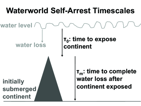
Figure 5.— Schematic diagram of the timescales involved in a waterworld self-arrest. $\tau_{0}$ is the time the planet exists in a moist greenhouse state before submerged continent is exposed. $\tau_{m}$ is the time to complete planetary water loss after the first exposure of continent. In order to determine whether a waterworld self-arrest is possible, $\tau_{m}$ must be compared with $\tau_{w}$, the timescale for CO₂ to be sufficiently reduced by silicate weathering that moist greenhouse conditions cease to exist.

$\tau_{w}$ is much more difficult to estimate than $\tau_{m}$. The closest known analog to a moist greenhouse in post-Hadean Earth is likely the aftermath of the Snowball Earth events, which occurred 600–700 million years ago. The dominant explanation for Snowball Earth events (Kirschvink, 1992; Hoffman et al., 1998) is that some cooling factor forced Earth into a global glaciation, which is an alternative stable state of climate because of the high reflectivity of snow and ice. Because it would be very cold during a Snowball and because any precipitation would fall as snow, rather than rain, the continental weathering rate would be near zero. As we expect volcanic CO₂ outgassing to continue unabated, the atmospheric CO₂ would increase until it reached up to a thousand times its present value ($\phi=\cal{O}$(10³)), at which point it would be warm enough to melt the ice and end the Snowball. In the immediate aftermath of a Snowball Earth event the planetary albedo would be very low and the CO₂ concentration would be very high, which would lead to surface temperatures in the range of a moist greenhouse. Extremely high weathering would then reduce the atmospheric CO₂ until Earth’s surface temperatures were comparable to modern values (Higgins & Schrag, 2003). If post-Snowball Earth was truly in a moist greenhouse state, complete water loss must not have occurred, which would imply that $\tau_{w}<\tau_{m}$ and a waterworld self-arrest is possible. Even if post-Snowball Earth was not a true moist greenhouse, the drawdown of CO₂ must have been immense, and geochronological evidence indicates that this took less than 4 Myr (Condon et al., 2005). This further motivates the idea that $\tau_{w}$ could be small compared to $\tau_{m}$.

The CO₂ required to end a Snowball Earth, however, may have been 1-2 orders of magnitude lower than that quoted above (Abbot & Pierrehumbert, 2010), in which case the Snowball aftermath would be a weaker analog for a moist greenhouse and further consideration is required. Geochemical modeling under conditions similar to a moist greenhouse yield weathering rates of $\cal{O}$($10^{13}$) kg C yr^-1 (Higgins & Schrag, 2003) and $\cal{O}$($10^{12}$) kg C yr^-1 (Le Hir et al., 2009), although Mills et al. (2011) suggest that ion transport constraints could limit the weathering rate to $\approx 5\times 10^{11}$ kg C yr^-1 (Mills et al., 2011). The waterworld CO₂ is $1.65\times 10^{4}$ times the present value (Figure 1) in our model with standard parameters, which corresponds to $\cal{O}$($10^{19}$ kg C). This yields an estimate of $\tau_{w}=\cal{O}$(1-10 Myr), which further suggests that $\tau_{w}<\tau_{m}$.

Although we have not performed a full analysis of the kinetic (non-equilibrium) effects, the order-of-magnitude analysis we have done indicates that a habitable zone waterworld could stop a moist greenhouse through weathering and become a habitable partially ocean-covered planet. We note that this process would not occur if the initial water complement of the planet is so large that continent is not exposed even after billions of years in the moist greenhouse state ($\tau_{0}>\cal{O}$(10 Gyr)). Additionally, we have neglected the possibility of water exchange between the mantle and the surface, which is poorly constrained on Earth. If, for some reason, water were continuously released from the planetary interior to replace water lost through hydrogen escape, then the conclusions reached here would be invalid. This would require significantly higher mantle-surface fluxes than on present Earth, which are constrained by cerium measurements at mid-ocean ridges to be small enough to require $\approx$10 Gyr to replace Earth’s surface water reservoir (Hirschmann & Kohlstedt, 2012). Finally, we note that since we have considered a moist greenhouse caused by high atmospheric optical thickness rather than high insolation, the waterworld would not be likely to suffer a full runaway greenhouse during the process described here (Nakajima et al., 1992).

6. Discussion of Observability

The theory developed here suggests that if an Earth-size planet is detected near the habitable zone it should be considered a good candidate to have a wide habitable zone and a long-term stable climate as long as it has some exposed land. The first observational point to consider, therefore, is whether the surface land fraction could be measured on an Earth-like planet.

Using measurements of the rotational variations of disk-integrated reflected visible light from a future mission such as TPF-C it will be possible to determine the surface land fraction of an Earth-like planet orbiting a Sun-like star. Cowan et al. (2009) used observations of Earth from the Deep Impact spacecraft to demonstrate that this is possible with multi-band high-cadence photometry. The multi-band observations are critical because the albedo of land and ocean have very different wavelength dependencies, while the integration times must be sufficiently short to resolve the planet’s rotational variability. Clouds tend to obscure surface features and make such a determination more difficult (Ford et al., 2001; Kaltenegger et al., 2007; Palle et al., 2008), and regions of a planet that are consistently cloudy are impervious to this form of remote sensing (Cowan et al., 2011). Kawahara & Fujii (2010, 2011) have extended this method to include seasonal changes in illumination to generate rough two-dimensional maps of otherwise unresolved planets. Provided that a habitable zone planet is not much cloudier than Earth, its land fraction should therefore be observationally accessible with sufficient signal-to-noise ratio, and the present study can be used to help assess the probability of its habitable zone width and long-term habitability.

The presence of exposed land could be detected on an exoplanet via an infrared emission spectrum, provided the overlying atmosphere is not too much of a hindrance (Hu et al., 2012). At thermal wavelengths, the land fraction of a planet could in principle be estimated based on its thermal inertia, but in idealized tests Gaidos & Williams (2004) found that the obliquity-inertia degeneracy impedes quantitative estimates of a planet’s heat capacity. It is therefore unlikely that a thermal mission, on its own, could constrain the land fraction of an exoplanet.

Direct confirmation or falsification of the theory developed here will be more difficult, requiring not only an estimate of land fraction, but also atmospheric CO₂ abundance and/or surface temperature. The difference between the temperature and CO₂ of a waterworld and a partially ocean-covered planet could be quite large, particularly near the inner (hotter) edge of the habitable zone (Figure 1). This entails measuring, in exoplanets, discrepancies in carbon dioxide abundance of roughly four orders of magnitude, and surface temperatures differences of $\sim 70$ K.

Detecting carbon dioxide in an exoplanet atmosphere is relatively easy: the James Webb Space Telescope will determine whether CO₂ is present in the atmospheres of transiting super-Earths orbiting M-stars (Deming et al., 2009; Kaltenegger & Traub, 2009; Belu et al., 2011; Rauer et al., 2011). The challenge is in estimating the amount of CO₂ in an atmosphere. In order to measure the carbon dioxide abundance of an atmosphere, the atmospheric mass must be estimated. This could be achieved for M-Dwarf habitable zone planets with transit spectroscopy covering the Rayleigh scattering slope (Benneke & Seager, 2012). The unknown radius of directly-imaged (longer-period) exoplanets may hinder such estimates with a TPF-C type mission. At thermal wavelengths, the planetary radius will be measurable and the pressure broadening of absorption features may offer an estimate of surface pressure and hence atmospheric mass (e.g., Des Marais et al., 2002; Meadows & Seager, 2010).

Using a thermal mission like TPF-I, it may be possible to determine the surface temperature of an Earth analog via its brightness temperature in molecular opacity windows, at least for a cloud-free atmosphere with few IR absorbers (Des Marais et al., 2002; Kaltenegger et al., 2010; Selsis et al., 2011). While low-lying clouds do not significantly degrade such estimates, high cloud coverage can lead to surface temperature estimates at least 35 K too low (Kaltenegger et al., 2007; Kitzmann et al., 2011). Continuum opacity from water vapor will also lead to lower brightness temperatures, even in opacity windows. This could lead to under-estimating the surface temperature of planets with high vapor content, precisely the moist greenhouse planets expected to have high surface temperatures. Moreover, Venus dramatically demonstrates that brightness temperatures, even in supposed windows, are not necessarily a good probe of the surface temperature.

Given the similar temperature and CO₂ among partially ocean-covered planets of varying land fraction (Figure 1), it is unlikely that any mission in the foreseeable future would be able to distinguish between them. Additionally, factors that we have neglected here introduce uncertainties that make the temperature and CO₂ abundance among partially ocean-covered planets effectively indistinguishable.

To summarize, measurements from a mission like TPF-C would provide a surface land fraction estimate for planets not much cloudier than Earth. TPF-C could provide an order-of-magnitude atmospheric CO₂ estimate if the radius were known, which would be possible if (1) the planet were transiting, (2) its radius were estimated from TPF-I observations, or (3) its radius were estimated based on a mass measurement. TPF-I could provide a surface temperature estimate that would likely be good to $\cal{O}$(10 K) for an Earth analog, but possibly much worse for a cloudier and/or more humid atmosphere. It would therefore be possible to directly test our predictions for differences in weathering behavior of waterworlds and partially ocean-covered planets if data from missions like both TPF-C and TPF-I were available, and sufficient numbers of nearby habitable zone planets exist. Prospects are limited, but testability is still possible in special cases (such as a transiting planet), if only one type of data is available.

A final observational point is that in Section 5 we calculated that a waterworld self-arrest, through which a fully ocean planet would be transformed into a partial ocean planet, is possible. Waterworlds, however, would still exist and their detection would not falsify the waterworld self-arrest idea. Waterworlds could have orders of magnitude more water than Earth (e.g., Raymond et al., 2007; Fu et al., 2010), and could therefore exist in a moist greenhouse state for many billions of years. Additionally, a waterworld in the outer regions of the habitable zone would not be in a moist greenhouse state (Figure 4).

7. General Discussion

We note again that we make numerous approximations in our model, so that it is useful for qualitative understanding rather than quantitative predictions. Our linearized climate model, for example, is a gross simplification of the real climate system, which is probably responsible for the delayed onset of the moist greenhouse in our model as the insolation is increased (Figure 1) relative to more detailed calculations (Kasting et al., 1993). Our approach, however, is appropriate for a general study of potential terrestrial exoplanets, whose detailed characteristics are not known, and our main conclusions should be robust to more detailed modeling. For example, we point out that no weathering feedback is possible ($\frac{\partial T}{\partial S}=\left(\frac{\partial T}{\partial S}\right)_{0}$) for a waterworld as long as seafloor weathering is independent of surface temperature ($T$), regardless of the specific form of the seafloor weathering parameterization.

Nonetheless, our parameterization of seafloor weathering is probably the most uncertain aspect of this work. For example, we have neglected the potential effect of a different ocean chemical composition on an exoplanet, which could lead to different base weathering rates or a different scaling of seafloor weathering with CO₂ ($\phi$). Furthermore, in order to derive a scaling relationship between [H⁺] and $\phi$, we have approximated ocean chemistry as a carbonate ion system with changes in alkalinity determined by changes in Ca²⁺. Real oceans have other ions present, which can alter the charge balance. These approximations, however, have been useful for modeling carbon cycling in deep time Earth problems (e.g., Higgins & Schrag, 2003) and our knowledge of typical ion concentrations in terrestrial exoplanets is unconstrained. Finally, we have assumed that surface temperature has a negligible effect on seafloor weathering rate, which we will now consider in more detail.

As there is a temperature dependence of the reactions relevant for seafloor weathering (Brady & Gislason, 1997), we have effectively assumed that surface temperature does not strongly affect the temperature at which seafloor weathering occurs. If a dependence of seafloor weathering on surface temperature is allowed, a climate-seafloor weathering feedback is possible, which should tend to reduce the effect of changing land fraction. In terms of the effect of land fraction on weathering behavior, we have therefore considered a conservative case in assuming no surface temperature dependence of seafloor weathering, yet we still found that land fraction has only a small effect on weathering behavior for partially ocean-covered planets.

A strong temperature dependence of seafloor weathering would affect waterworld behavior at the inner edge of the habitable zone. We can see this by multiplying the seafloor weathering parameterization (Equation (7)) by an exponential temperature dependence of the form $e^{\eta T}$, where $\eta=\frac{dT_{u}}{T_{w}}$, where $d$ is the change in seafloor weathering reaction temperature per unit change in surface temperature, and $T_{w}\approx 15$K is the exponential scale of increase in seafloor weathering reaction rate with temperature (Brady & Gislason, 1997). The largest value $\eta$ could take would be if current reactions occur near the bottom water temperature ($\approx$0^∘C) and each unit increase in surface temperature creates a unit increase in bottom water temperature ($d$=1, $\eta=\frac{2}{3}$). Our standard assumption is that seafloor weathering reactions occur at a temperature of $\approx$20-40^∘C regardless of surface temperature, which is equivalent to $d$=$\eta$=0. Using $\eta=\frac{2}{3}$ increases the insolation required to cause a waterworld moist greenhouse from $S$$\approx$1.2 to $S$$\approx$2.1 if $\nu$=0 and prevents a waterworld moist greenhouse from ever happening if $\nu$=12.6. A strong temperature dependence of seafloor weathering would therefore make it much harder for a waterworld to experience a moist greenhouse, although we do not consider the limiting case considered in this paragraph likely.

As noted in Section 2, we assume that seafloor spreading produces a sufficient quantity of weatherable material and a sufficient amount of water can circulate through it that the seafloor weathering rate can increase arbitrarily as the ocean pH decreases. Since we assume seafloor weathering accounts for 25% of weathering on modern Earth ($\beta_{0}=0.75$), if the CO₂ outgassing rate takes its modern value ($\Gamma=1$), then the seafloor weathering rate must be able to increase by a factor of four if it alone is to balance outgassing, as would be required to establish a CO₂ steady state on a waterworld. If there is not enough weatherable material for this to be possible, for example due to weak circulation of seawater through weatherable material, then the waterworld CO₂ will not be limited to the value calculated in Section 3 (Figure 1), but will instead steadily increase due to an unbalanced source and sink. This would push a waterworld more quickly to a moist greenhouse, and potentially a waterworld self-arrest, than one would otherwise expect. A related issue is that if the land fraction is very small, there may be physical limits on continental weathering not included in Equation (3). This would lead to higher CO₂ concentrations and temperatures for small land fractions than those found in Section 3. The smallest land fraction we explicitly considered, however, was $\gamma=0.01$, which corresponds to the combined area of Greenland and Mexico on Earth. Given continuous resurfacing it is not clear that physical limitations on weathering would be in play on such a large land area.

We have focused on the effect on land fraction on weathering behavior relevant for the broad interior of the habitable zone and the evolution of a planet through the habitable zone over time. The effect of land fraction on the outer (cold) edge of the habitable zone is of interest as well. Based on increased Rayleigh scattering or CO₂ condensation at the surface, the outer edge of the habitable zone occurs when CO₂$\approx$5–10 bar (Kasting et al., 1993). Le Hir et al. (2008), however, found that seafloor weathering should limit the maximum CO₂ concentration on Earth to a few tenths of a bar. As pointed out by Pierrehumbert (2011), if this is the case, then the CO₂ condensation limit could not be reached and seafloor weathering would shrink the habitable zone. Using our seafloor weathering parameterization, we can derive an upper limit on the atmospheric CO₂ concentration with Earth’s land fraction ($\gamma=\gamma_{0}$): $\bar{\phi}=\left(\frac{\Gamma(1+\nu)}{(1-\beta_{0})}-\nu\right)^{\frac{1}{n}}$. Using our standard parameters, we find $\bar{\phi}=7.3\times 10^{4}$, or $\approx$20 bar. $\bar{\phi}$ depends strongly, however, on model parameters (Figure 6), particularly $n$. $\bar{\phi}=10^{3}$, roughly the value Le Hir et al. (2008) found, would be produced by our model by either a change in $n$ from 0.33 to 0.54 or a change in $\nu$ from 12.6 to 2.0. Therefore, in contrast to our main results (Section 4), the weathering behavior relevant for the outer edge of the habitable zone is highly sensitive to the seafloor weathering parameterization. A convincing study of the effect of seafloor weathering on the outer edge of the habitable zone will have to wait until seafloor weathering is better understood.

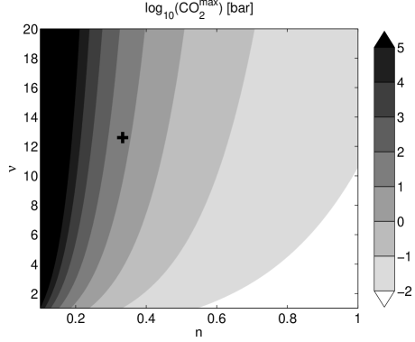
Figure 6.— Maximum atmospheric partial pressure of CO₂ (dimensionful version of $\bar{\phi}$) allowed by seafloor weathering, as a function of $n$ and $\nu$, parameters in the seafloor weathering scheme (Equation (7)). The “+” represents standard parameter values.

We have found that relatively ineffective seafloor weathering will tend to lead to much warmer temperatures in a waterworld than a partial ocean planet. This might appear to contrast with Sleep & Zahnle (2001), who calculated very cold temperatures for Earth during the Hadean, when Earth had a much lower land fraction and was further out in the habitable zone. The primary reason for the difference is that Sleep & Zahnle (2001) include a significant sink of carbon due to weathering of impact ejecta during the Hadean, which significantly reduces the equilibrated CO₂ and temperature. They also assume that seafloor weathering is much more active due to increased internal heat flux early in Earth’s history. We do not include either of these effects because our effort is aimed at general consideration of the problem in the context of exoplanets, but we acknowledge that either could limit the CO₂, and therefore the probability of a moist greenhouse, on a waterworld. Finally, Sleep & Zahnle (2001) also find a strong dependence of equilibrated CO₂ on the strength of the CO₂ dependence of seafloor weathering, as we do (Figure 6), early in Earth’s history when the CO₂ may have been very high. This again emphasizes that the details of the seafloor weathering scheme are critical for its effect on the outer edge of the habitable zone, or equivalently the climate of early Earth.

In our analysis we set the planetary albedo to a constant for simplicity. Since the albedo of land (0.05-0.3, Peixoto & Oort, 1992) tends to be higher than the albedo of ocean (0.05-0.1, Peixoto & Oort, 1992), one would expect the planetary albedo to increase as the land fraction increases. This would decrease the temperature (T, Equation (11)) and the climate sensitivity to external forcing ($\frac{\partial T}{\partial S}$, Equation (16)), both of which we found would already be lower due to more continental weathering (Section 3). This effect would likely not be very large, however, as detailed analysis of satellite measurements indicates that because of extensive absorption and reflection by clouds and gas in the atmosphere the surface contributes only $\cal{O}$(10%) to the global mean albedo on Earth (Donohoe & Battisti, 2011). The influence of surface albedo on planetary albedo would be further reduced around M stars, which emit at longer wavelengths, due to increased atmospheric scattering and absorption (Kasting et al., 1993). Another surface albedo effect we have neglected is the change in albedo in colder climates due to the formation of ice and snow at the surface. This would lead to a reduction in the range of $S$ for which a planet is habitable in Figure 1. Again, however, this effect would be reduced around M stars due to greatly reduced ice and snow albedos (Joshi & Haberle, 2011).

Our model neglects spatial variation in climate and weathering, and therefore cannot address spatially heterogeneous effects such as the feedbacks described by Kite et al. (2011). An assumption of spatial homogeneity, however, is a reasonable first approximation even on planets with highly asymmetric insolation distributions, such as tidally locked planets in the habitable zone of M stars, if there is an ocean or atmosphere similar in size to those on Earth to redistribute heat (e.g., Joshi et al., 1997; Merlis & Schneider, 2010; Edson et al., 2011).

Current understanding is that continents were not present at Earth’s formation, but started to form soon afterward. For example, zircon evidence indicates that there was continental crust 4.4 Gyr ago, or within $\approx$100 Myr of Earth’s formation (Wilde et al., 2001). Available evidence cannot constrain whether the continents reached their present size quickly (within $\approx$500 Myr) or have grown slowly over Earth’s history and continue to grow today (Eriksson et al., 2006). We have neglected such processes, but this is unlikely to modify our main conclusions because we found that the climate sensitivity to external forcing ($\frac{\partial T}{\partial S}$) does not depend strongly on land fraction. Our work suggests that the order of magnitude of water delivery, which determines whether a planet is dry, partially ocean-covered, or a waterworld, is much more important for determining weathering behavior than evolution in the size of continents through a planet’s lifetime. Finally, it is worth speculating that Earth could have experienced a waterworld self-arrest early in its history, although much more thought is needed to determine what the geochemical signals left behind by such an event would be.

If a waterworld has a thick enough ocean, the overburden pressure could significantly suppress volcanic outgassing. For example, CO₂ degassing could be completely suppressed on an Earth-like planet with 100 km of ocean (Kite et al., 2009). This uncertainty is commensurate with other volcanic outgassing uncertainties, such as CO₂ content in the magma, for partial ocean planets and waterworlds that barely cover their continents with ocean. Overburden outgassing suppression could lead to lower CO₂ levels and higher chance of a Snowball state than predicted here for waterworlds with a thick ocean layer.

In our discussion of a waterworld self-arrest (Section 5) we neglected effects of changing planetary size. Super-Earths would have higher gravity and therefore reduced orography. This will reduce the amount of time it takes from first exposure of land to complete water loss ($\tau_{m}$), which will make a waterworld self-arrest less likely. On the other hand, the higher gravity of a super-Earth will also make gas escape from the atmosphere to space more difficult, which would reduce $\tau_{m}$. Full consideration of a waterworld self-arrest on a super-Earth is beyond the scope of this paper.

8. Conclusions

We have shown that using standard weathering parameterizations, the weathering behavior of a partially ocean-covered Earth-like planet does not depend strongly on land fraction, as long as the land fraction is greater than $\approx$0.01. Consequently, planets with some continent and some ocean should have a habitable zone of similar width. This is a powerful result because it indicates that previous habitable zone theory developed assuming Earth-like land fraction and weathering behavior should be broadly applicable.

We have also pointed out that, as long as seafloor weathering does not depend directly on surface temperature, a climate-weathering feedback cannot operate on a waterworld. This is a significant result because it would imply that waterworlds have a much narrower habitable zone than a planet with even a few small continents. We find, however, that weathering could operate quickly enough that a waterworld could “self-arrest” while undergoing a moist greenhouse and the planet would be left with partial ocean coverage and a clement climate. If this result holds up to more detailed kinetic weathering modeling, it would be profound, because it implies that waterworlds that form in the habitable zone have a pathway to evolve into a planet with partial ocean coverage that is more resistant to changes in stellar luminosity.

9. Acknowledgements

We thank Jens Teiser for suggesting that we consider whether weathering could draw down CO₂ fast enough to stop a moist greenhouse and David Archer and Ray Pierrehumbert for fruitful discussions early in the development of this project. We acknowledge input from Francis MacDonald on Snowball geochronology, John Higgins on weathering parameterizations, and Bob Wordsworth on the effect of CO₂ clouds on the habitable zone. Jacob Bean, Albert Colman, Itay Halevy, Guillaume Le Hir, Edwin Kite, Daniel Koll, Arieh Konigl, and an anonymous reviewer provided helpful comments on early drafts of this paper. We thank Björn Benneke for sharing an early draft of his manuscript.

References

- Abbot & Pierrehumbert (2010) Abbot, D. S., & Pierrehumbert, R. T. 2010, J. Geophys. Res., 115, D03104
- Abbot et al. (2011) Abbot, D. S., Voigt, A., & Koll, D. 2011, J. Geophys. Res., 116, D18103
- Abe et al. (2011) Abe, Y., Abe-Ouchi, A., Sleep, N. H., & Zahnle, K. J. 2011, Astrobiology, 11, 443
- Anglada-Escudé et al. (2012) Anglada-Escudé, G., et al. 2012, ApJ, accepted (arXiv:1202.0446)
- Belu et al. (2011) Belu, A. R., Selsis, F., Morales, J.-C., et al. 2011, A&A, 525, A83
- Benneke & Seager (2012) Benneke, B., & Seager, S. 2012, ApJ, 753, 100
- Berner (1994) Berner, R. 1994, Am J Sci, 294, 56
- Berner (2004) Berner, R. A. 2004, The Phranerozoic Carbon Cycle (New York: Oxford Univ. Press)
- Bloh et al. (2005) Bloh, W. V., Bounama, C., & Franck, S. 2005, Celest. Mech. Dyn. Astr., 92, 287
- Borucki et al. (2011) Borucki, W. J., et al. 2011, ApJ, 745, 120
- Brady & Gislason (1997) Brady, P., & Gislason, S. 1997, Geochim. Cosmochim. Acta, 61, 965
- Caldeira (1995) Caldeira, K. 1995, Am J Sci, 295, 1077
- Caldeira & Kasting (1992) Caldeira, K., & Kasting, J. 1992, Nature, 360, 721
- Condon et al. (2005) Condon, D., Zhu, M. Y., Bowring, S. et al. 2005, Science, 308, 95
- Cowan et al. (2009) Cowan, N. B., Agol, E., Meadows, V.S. 2009, ApJ, 700, 915
- Cowan et al. (2011) Cowan, N. B., Robinson, T., Livengood, T. A., et al. 2011, ApJ, 731, 76
- Deming et al. (2009) Deming, D., Seager, S., Wigg, J., et al. 2009, PASP, 121, 952
- Des Marais et al. (2002) Des Marais, D. J., Harwit, M. O., Jucks, K. W. et al. 2002, Astrobiology, 2, 153
- Donohoe & Battisti (2011) Donohoe, A., & Battisti, D. S. 2011, J. Clim., 24, 4402
- Drever (1988) Drever, J. I. 1988, The Geochemistry of Natural Waters (Englewood Cliffs, JJ: Prentice-Hall), 437
- Dunne (1978) Dunne, T. 1978, Nature, 274, 244
- Edson et al. (2011) Edson, A., Lee, S., Bannon, P., Kasting, J. F., & Pollard, D. 2011, Icarus, 212, 1
- Eriksson et al. (2006) Eriksson, P. G., Mazumder, R., Catuneanu, O., Bumby, A. J., & Ilondo, B. O. 2006, Earth-Sci Rev, 79, 165
- Feulner (2012) Feulner, G. 2012, Rev. Geophys., 50
- Ford et al. (2001) Ford, E., Seager, S., & Turner, E. 2001, Nature, 412, 885
- Forget & Pierrehumbert (1997) Forget, F., & Pierrehumbert, R. T. 1997, Science, 278, 1273
- Forget et al. (2012) Forget, F., Wordsworth, R. D., Millour, E., Madeleine, J.-B., & Charnay, B. 2012, Icarus, submitted
- Fu et al. (2010) Fu, R., O’Connell, R. J., & Sasselov, D. D. 2010, ApJ, 708, 1326
- Gaidos & Williams (2004) Gaidos, E., & Williams, D. 2004, New Astron., 10, 67
- Gough (1981) Gough, D. O. 1981, Sol. Phys., 74, 21
- Higgins & Schrag (2003) Higgins, J. A., & Schrag, D. P. 2003, Geochem. Geophys. Geosyst., 4, 1028
- Hirschmann & Kohlstedt (2012) Hirschmann, M., & Kohlstedt, D. 2012, Phys Today, 65, 40
- Hoffman et al. (1998) Hoffman, P. F., Kaufman, A. J., Halverson, G. P., & Schrag, D. P. 1998, Science, 281, 1342
- Hu et al. (2012) Hu, R., Ehlmann, B. L., & Seager, S. 2012, ApJ, 752, 7
- Joshi & Haberle (2011) Joshi, M., & Haberle, R. 2011, Astrobiology, 12, 3
- Joshi et al. (1997) Joshi, M., Haberle, R., & Reynolds, R. 1997, Icarus, 129, 450
- Kaltenegger & Sasselov (2011) Kaltenegger, L., & Sasselov, D. 2011, ApJ, 736, L25
- Kaltenegger & Traub (2009) Kaltenegger, L., & Traub, W. A. 2009, ApJ, 698, 519
- Kaltenegger et al. (2007) Kaltenegger, L., Traub, W. A., & Jucks, K. W. 2007, ApJ, 658, 598
- Kaltenegger et al. (2011) Kaltenegger, L., Udry, S., & Pepe, F. 2011, A&A, submitted (arXiv:1108.3561)
- Kaltenegger et al. (2010) Kaltenegger, L., Selsis, F., Fridlund, M., et al. 2010, Astrobiology, 10, 89
- Kasting (2010) Kasting, J. F. 2010, Nature, 464, 687
- Kasting et al. (1993) Kasting, J. F., Whitmire, D. P., & Reynolds, R. T. 1993, Icarus, 101, 108
- Kawahara & Fujii (2010) Kawahara, H., & Fujii, Y. 2010, ApJ, 720, 1333
- Kawahara & Fujii (2011) Kawahara, H., & Fujii, Y. 2011, ApJ, 739, L62
- Kirschvink (1992) Kirschvink, J. 1992, in The Proterozoic Biosphere: A Multidisciplinary Study, ed. J. Schopf & C. Klein (New York: Cambridge Univ. Press), 51
- Kite et al. (2011) Kite, E., Gaidos, E., & Manga, M. 2011, ApJ, 743, 41
- Kite et al. (2009) Kite, E., Manga, M., & Gaidos, E. 2009, ApJ, 700, 1732
- Kitzmann et al. (2011) Kitzmann, D., Patzer, A. B. C., von Paris, P., Godolt, M., & Rauer, H. 2011, A&A, 531, A62
- Kuchner (2003) Kuchner, M. J. 2003, ApJ, 596, L105
- Le Hir et al. (2009) Le Hir, G., Donnadieu, Y., Godderis, Y., et al. 2009, Earth Planet. Sci. Lett., 277, 453
- Le Hir et al. (2008) Le Hir, G., Ramstein, G., Donnadieu, Y., & Godderis, Y. 2008, Geology, 36, 47
- Marshall et al. (1988) Marshall, H., Walker, J., & Kuhn, W. 1988, J. Geophys. Res., 93, 791
- Mayor et al. (2009) Mayor, M., Bonfils, X., Forveille, T. et al. 2009, A&A, 507, 487
- Meadows & Seager (2010) Meadows, V., & Seager, S. 2010, in Exoplanets, ed. S. Seager (Tucson, AZ: The University of Arizona Press), 441
- Merlis & Schneider (2010) Merlis, T., & Schneider, T. 2010, Journal of Advances in Modeling Earth Systems, 2, 13
- Meybeck (1979) Meybeck, M. 1979, Rev. Géol. Dyn. Géogr. Phys., 21, 215
- Mills et al. (2011) Mills, B., Watson, A. J., Goldblatt, C., Boyle, R., & Lenton, T. M. 2011, Nature Geosci., 4, 861
- Mischna et al. (2000) Mischna, M. A., Kasting, J. F., Pavlov, A., & Freedman, R. 2000, Icarus, 145, 546
- Morbidelli et al. (2000) Morbidelli, A., Chambers, J., Lunine, J. I., et al. 2000, Meteorit. Planet. Sci., 35, 1309
- Nakajima et al. (1992) Nakajima, S., Hayashi, Y. Y., & Abe, Y. 1992, J. Atmos. Sci., 49, 2256
- O’Brien et al. (2006) O’Brien, D. P., Morbidelli, A., & Levison, H. F. 2006, Icarus, 184, 39
- O’Gorman & Schneider (2008) O’Gorman, P. A., & Schneider, T. 2008, J. Cli., 21, 3815
- Palle et al. (2008) Palle, E., Ford, E. B., Seager, S., Montanes-Rodriguez, P., & Vazquez, M. 2008, ApJ, 676, 1319
- Peixoto & Oort (1992) Peixoto, J. P., & Oort, A. H. 1992, Physics of Climate (New York: AIP), 520
- Pepe et al. (2011) Pepe, F., Lovis, C., Ségransan, D. et al. 2011, A&A, 534, A58
- Peters (1984) Peters, N. 1984, U.S. Geol. Surv. Water Supply Pap. 2228, 39
- Pierrehumbert & Gaidos (2011) Pierrehumbert, R., & Gaidos, E. 2011, ApJ, 734, L13
- Pierrehumbert (2010) Pierrehumbert, R. T. 2010, Principles of Planetary Climate (Cambridge: Cambridge Univ. Press)
- Pierrehumbert (2011) Pierrehumbert, R. T. 2011, ApJ, 726, L8
- Rauer et al. (2011) Rauer, H., Gebauer, S., Paris, P. V. et al. 2011, A&A, 529, A8
- Raymond (2006) Raymond, S. N. 2006, ApJ, 643, L131
- Raymond et al. (2009) Raymond, S. N., O’Brien, D. P., Morbidelli, A., & Kaib, N. A. 2009, Icarus, 203, 644
- Raymond et al. (2007) Raymond, S. N., Scalo, J., & Meadows, V. S. 2007, ApJ, 669, 606
- Sagan & Mullen (1972) Sagan, C., & Mullen, G. 1972, Science, 177, 52
- Schaefer & Fegley (2010) Schaefer, L., & Fegley, B. 2010, Icarus, 208, 438
- Schneider et al. (2010) Schneider, T., O’Gorman, P. A., & Levine, X. J. 2010, Rev. Geophys., 48, RG3001
- Selsis et al. (2007) Selsis, F., Kasting, J. F., Levrard, B. et al. 2007, A&A, 476, 1373
- Selsis et al. (2011) Selsis, F., Wordsworth, R. D., & Forget, F. 2011, A&A, 532, A1
- Sleep & Zahnle (2001) Sleep, N. H., & Zahnle, K. 2001, J. Geophys. Res., 106, 1373
- Udry et al. (2007) Udry, S., Bonfils, X., Delfosse, X. et al. 2007, A&A, 469, L43
- Vogt et al. (2010) Vogt, S. S., Butler, R. P., Rivera, E. J., et al. 2010, ApJ, 723, 954
- Voigt et al. (2011) Voigt, A., Abbot, D. S., Pierrehumbert, R. T., & Marotzke, J. 2011, Clim. Past, 7, 249
- Walker et al. (1981) Walker, J., Hays, P., & Kasting, J. 1981, J. Geophys. Res., 86, 9776
- Watson et al. (1981) Watson, A., Donahue, T., & Walker, J. 1981, Icarus, 48, 150
- Wilde et al. (2001) Wilde, S. A., Valley, J. W., Peck, W. H., & Graham, C. M. 2001, Nature, 409, 175
- Wordsworth (2012) Wordsworth, R. 2012, Icarus, 219, 267
- Wordsworth et al. (2012) Wordsworth, R. D., Forget, F., Millour, E., and Head, J.-B. M., & Charnay, B. 2012, Icarus, submitted
- Wordsworth et al. (2011) Wordsworth, R. D., Forget, F., Selsis, F., et al. 2011, ApJ, 733, L48
- Yang et al. (2012) Yang, J., Peltier, W., & Hu, Y. 2012, J. Cli., 25, 2711