Swarm-NG: a CUDA Library for Parallel  $n$-body Integrations with focus on Simulations of Planetary Systems

Abstract

We present Swarm-NG, a C++ library for the efficient direct integration of many  $n$-body systems using a Graphics Processing Unit (GPU), such as NVIDIA’s Tesla T10 and M2070 GPUs. While previous studies have demonstrated the benefit of GPUs for  $n$-body simulations with thousands to millions of bodies, Swarm-NG focuses on many few-body systems, e.g., thousands of systems with 3…15 bodies each, as is typical for the study of planetary systems. Swarm-NG parallelizes the simulation, including both the numerical integration of the equations of motion and the evaluation of forces using NVIDIA’s “Compute Unified Device Architecture” (CUDA) on the GPU. Swarm-NG includes optimized implementations of 4th order time-symmetrized Hermite integration and mixed variable symplectic integration, as well as several sample codes for other algorithms to illustrate how non-CUDA-savvy users may themselves introduce customized integrators into the Swarm-NG framework. To optimize performance, we analyze the effect of GPU-specific parameters on performance under double precision. For an ensemble of 131072 planetary systems, each containing 3 bodies, the NVIDIA Tesla M2070 GPU outperforms a 6-core Intel Xeon X5675 CPU by a factor of $\sim 2.75$. Thus, we conclude that modern GPUs offer an attractive alternative to a cluster of CPUs for the integration of an ensemble of many few-body systems.

Applications of Swarm-NG include studying the late stages of planet formation, testing the stability of planetary systems and evaluating the goodness-of-fit between many planetary system models and observations of extrasolar planet host stars (e.g., radial velocity, astrometry, transit timing). While Swarm-NG focuses on the parallel integration of many planetary systems, the underlying integrators could be applied to a wide variety of problems that require repeatedly integrating a set of ordinary differential equations many times using different initial conditions and/or parameter values.

1 Introduction

1.1 Background

An  $n$-body simulation numerically approximates the evolution of a system of bodies in which each body continuously interacts with every other body, a fundamental component of many physical and chemical systems.  $n$-body simulations are ubiquitous in astrophysics and planetary science. Example applications include investigating the trajectories of spacecraft, the formation and orbital evolution of the solar system and other planetary systems, the delivery of water to Earth via collisions with asteroids and/or comets, the evolution of star clusters, the formation of galaxies and even the evolution of the entire universe.

Given the widespread use of  $n$-body simulations, astronomers have developed a variety of algorithms and computer programs for performing  $n$-body integrations. At its core, an  $n$-body simulation requires solving a set of $3\times\mbox{$n$}$  second-order ordinary differential equations (ODEs). For $\mbox{$n$}\geq 3$, most sets of initial conditions result in chaotic evolution and are best studied numerically. The computational requirements of  $n$-body simulations can be significant, either due to long timescales (e.g., billions of years), a large number of bodies (e.g., $\sim 10^{5\ldots 7}$ for star cluster, $>10^{9}$ for galaxy or universe), and/or the need to consider a large number of systems with slightly different initial conditions (e.g., $\sim 10^{6\ldots 9}$ model evaluations for Bayesian analysis of exoplanet observations).

Several previous studies have demonstrated that the combination of modern Graphical Processing Unit (GPU) hardware and the CUDA (Compute Unified Device Architecture) programming environment can greatly accelerate a gravitational  $n$-body problem for large $n$ (e.g., star clusters) [2, 3, 6, 14, 18, 23, 24, 26]. Here we focus on the problem of integrating an ensemble of many few-body systems, e.g., thousands to millions of systems with 3 to tens of bodies each, as is needed for the study of planetary systems.

Given the large number of integrations of few-body systems, GPUs can dramatically reduce the total time required to obtain scientific results for many real-world applications (§6.2).

In this paper, we present the Swarm-NG library for parallel integration of  $n$-body systems. In §2, we describe the physical setup and the numerical methods. In §3, we describe key aspects of GPU computing with CUDA. In §4, we discuss the details of our implementations. In §5, we present performance benchmarks. In §6, we discuss present and likely applications.

2 Physics and Numerics of  $n$-body systems

2.1 Physics

The time evolution of a classical system of $n$ bodies is described by Newton’s laws of motion, ${\bf F_{i}}=m_{\bf i}{\bf a_{i}}$, where ${\bf a_{i}}$ is the acceleration vector (second time derivative of the position vector, ${\bf x_{i}}$) for the $i$th body, ${\bf F_{i}}$ is the gravity force of other bodies on the $i$th body and $m_{\bf i}$ is the mass of the $i$th body. Swarm-NG integrates systems interacting under Newtonian gravity,

$${\bf a_{i}}=\sum_{j\neq~{}i}\frac{Gm_{j}({\bf x_{j}}-{\bf x_{i}})}{\left|{\bf x_{j}}-{\bf x_{i}}\right|^{3}},$$ (1)

where $m_{j}$ is the mass of the $j$th body and $G$ is Newton’s Gravitational constant. Without loss of generality, we set $G=1$. If we use the astronomical unit (AU) as the unit of length and the solar mass ($M_{\odot}$) as the unit of mass, then one year corresponds to $2\pi$ time units. The modular design of Swarm-NG allows for the Newtonian force law to be replaced with an alternative force law, should users want to include additional effects such as general relativity, precession due to oblateness, or gas drag.

2.2 Numerical Integration of ODEs

For numerical integration, we replace the system of 3$\times$$n$ second-order differential equations by 6$\times$$n$ first-order differential equations,

$${\bf\dot{v_{i}}} ={\bf a_{i}}$$

$${\bf\dot{x_{i}}} ={\bf v_{i}},$$ (2)

where ${\bf v_{i}}$ is the velocity of the $i$th body.

There are a variety of methods for numerically integrating (2). The simplest, Euler integration given by

$${\bf{v_{i}}}(t+\Delta t) :={\bf{v_{i}}}(t)+{\bf a_{i}}(t)\Delta t,$$

$${\bf{x_{i}}}(t+\Delta t) :={\bf{x_{i}}}(t)+{\bf v_{i}}(t)\Delta t+\frac{1}{2}{\bf a_{i}}(t){\Delta t}^{2},$$

is however famously unstable and not practical for scientific simulations. Swarm-NG provides several advanced integration algorithms. The Hermite (§2.2.1) and Mixed Variables Symplectic (MVS; §2.2.3) integrators are currently the workhorse for scientific short-term and long-term integrations, respectively. Other integrators (e.g., Verlet, Runge-Kutta, modified midpoint method) have been implemented in Swarm-NG to compare their efficiency when using GPUs and to ensure that the Swarm-NG framework is sufficiently general to accommodate a variety of complex integration algorithms.

The Swarm-NG libraries are designed so that advanced users can quickly implement a new integration algorithm by writing code to advance the system by one time-step (i.e., a “propagator” class). They can then decide whether to write a more efficient but less generic and more complicated “integrator” class, where user has more control over the overall algorithm. Converting the Hermite propagator into a Hermite integrator class resulted in more complex code and four additional lines of code, but provided a performance gain of up to 5%, depending on ensemble parameters.

While our implementation of these algorithms on the GPU is original, the underlying integration algorithms are the same as the corresponding standard CPU-based integrators. Therefore, readers may consult standard texts and references on the accuracy and stability of each algorithm to determine which algorithms are appropriate for their scientific problem.

2.2.1 Hermite

The fourth-order, time-symmetric Hermite integrator is described in [17]. Like a standard Hermite integrator, it uses analytic expressions to calculate both the acceleration and ${\bf j}:=\dot{\bf a}$, the “jerk” (time derivative of the acceleration). Each Hermite step consists of a prediction step,

$${\bf x_{1}} :={\bf x_{0}}+{\bf v_{0}}\Delta t+\frac{1}{2}{\bf a_{0}}(\Delta t)^{2}+\frac{1}{6}{\bf j_{0}}(\Delta t)^{3}$$

$${\bf v_{1}} :={\bf v_{0}}+{\bf a_{0}}\Delta t+\frac{1}{2}{\bf j_{0}}(\Delta t)^{2},$$ (3)

followed by one or more correction steps,

$${\bf x_{k+1}} :={\bf x_{k}}-\frac{3}{10}\left({\bf a_{0}}-{\bf a_{k}}\right)(\Delta t)^{2}-\frac{1}{60}\left(7{\bf j_{0}}+2{\bf j_{k}}\right)(\Delta t)^{3}$$

$${\bf v_{k+1}} :={\bf v_{0}}-\frac{1}{2}\left({\bf a_{0}}-{\bf a_{k}}\right)\Delta t-\frac{1}{12}\left(5{\bf j_{0}}+{\bf j_{k}}\right)(\Delta t)^{2},$$ (4)

where the ${\bf a_{k}}$ and ${\bf j_{k}}$ are recalculated based on ${\bf x_{k}}$. Following [17], Swarm-NG’s Hermite integrator stops after two iterations of the correction step.

We implement two versions of the Hermite integrator, one with a fixed time-step and one with an adaptive time-step (see §4.3.1). Swarm-NG also includes a CPU-based Hermite integrator (fixed time step only), allowing for direct comparisons of CPU and GPU performance for this algorithm.

2.2.2 Runge-Kutta

Swarm-NG provides a fourth/fifth-order Runge-Kutta Cash-Karp integrator closely based on the gsl_odeiv2_step_rkck stepper from the GNU Science Library. We implemented two versions of the Runge-Kutta integrator, one with a fixed time-step and one with an adaptive time-step (see §4.3.2). The Runge-Kutta integrator uses only the accelerations and not the jerk. In order to achieve fifth order accuracy, the integrator estimates higher derivatives numerically. Therefore, both versions of the Runge-Kutta integrator require six sub-steps and six force evaluations for each step (fixed time-step) or trial step (adaptive time-step). Thus, this integrator is significantly more computationally expensive and memory intensive than the Hermite integrator. Its primary advantage is that only the acceleration needs to be specified. This makes it is easier to use with alternative force laws, when deriving an analytic expression for the jerk is not practical.

2.2.3 Mixed-Variable Symplectic

The Mixed-Variable Symplectic (MVS) integrator is optimized for integrating systems containing one dominant central body (e.g., star) and several small mass bodies (e.g., planets). Technically, it is not based on integrating the exact equations of motion, but rather the evolution of a map which has very similar properties to the actual equations of motion. The theory of the MVS integrator [30] is beyond the scope of this paper. We provide only an overview of the calculations and the essential properties so that readers can begin to understand the parallelization and judge whether MVS is an appropriate integrator for their problem.

Each step of the MVS integrator requires three kinds of sub-steps. To minimize the error due to the symplectic nature of the algorithm, the sub-steps are broken in half steps and calculated symmetrically as:

• Cartesian drift half step

• Kick half step

• Keplerian drift step

• Kick half step

• Cartesian drift half step

In the Cartesian drift half steps, the position of the center of mass is advanced based on the current center-of-mass velocity and the position of each planet relative to the central body is advanced due to the reflex motion of the central body in response to all of the planets.
In the Interaction or Kick half steps, the velocities of each planet are advanced based on the acceleration due to the mutual gravitational interaction of the planets (while excluding the acceleration due to gravity between each planet and the central body).
In the Keplerian drift step, the positions and velocities of each planet are evolved along a Keplerian orbit (i.e., elliptical path with a non-uniform speed given by Kepler’s third law of planetary motion) corresponding to the trajectory of the planet if it were not being perturbed by any other planets.

As the name suggests, the MVS integrator makes use of multiple parameterizations of the system state. There is a one-to-one mapping between Cartesian coordinates and Keplerian orbital parameters (e.g., [22]). Using the two sets of variables makes each sub-step extremely simple. For example, the $i$th planet can be advanced exactly along a Keplerian orbit for an arbitrary $\Delta t$ simply by increasing the mean anomaly by $\frac{2\pi\Delta t}{P_{i}}$, where $P=\left(\frac{G(m_{0}+m_{i})}{a_{i}^{3}}\right)^{\frac{1}{2}}$ is the orbital period, $a_{i}$ is the semi-major axis, $m_{0}$ is the mass of the central body and $m_{i}$ is the planet mass. The work of the MVS integrator is dominated by converting between the two representations of the system. For few-body systems, the coordinate conversions can even require more computation than the force calculation. The most expensive part of the conversion is iteratively solving Kepler’s equation that relates the orbit in space to the orbit in time. Swarm-NG adopts a previously developed CUDA kernel for repeatedly solving Kepler’s equation on the GPU [12].

While the MVS integrator is only second-order in the time step, the error term for the integration is also proportional to the ratio of the planet masses to the central mass. The Keplerian drift sub-step evolves planets along Keplerian orbits, allowing accurate integrations even for large time-steps. If there were no mutual planetary perturbations then one could use an arbitrarily long time-step and still maintain accuracy to machine precision. Even more importantly, the MVS integrator is symplectic, resulting in excellent long-term energy conservation and only linear growth in the error of the orbital phase. This makes the MVS integrator very well suited for long-term integrations of planetary systems (e.g., testing for long-term stability).

The main drawback of MVS is that, to maintain the symplectic nature, a fixed time-step is required. This makes the MVS integrator inappropriate for evolving systems through close encounters, which would require either an adaptive time-step scheme or an unrealistically small fixed time-step.

3 The NVIDIA CUDA Architecture

A GPU offers between 5 and 30 multiprocessors with Single Instruction, Multiple Thread (SIMT) architecture. A kernel is a portion of an application program, compiled to the instruction set of the GPU and loaded to the GPU for execution on one or more multiprocessors. To achieve high parallelism, the kernel is launched on a large number of compute threads, each operating on its own set of data. Threads are organized into a grid of thread blocks, each containing $n_{\rm blocksize}$ threads. CUDA-capable GPUs have an on-chip shared memory with very fast general read and write access, approximately as fast as on-chip registers. This memory is shared among threads within the same block. The local and global memory space are implemented as read-write regions of device memory which has high throughput, but also high latency. While this memory is not cached on earlier generations of GPUs (before Fermi), recent GPU architectures (Fermi and Kepler) include a two level cache mechanism; see Table 2. Still, the high computational throughput means that memory access can easily become the bottleneck.

3.1 Challenges of GPU Computing

GPU memory is arranged in different memory spaces, e.g., the latency of accessing global memory is about 100 times that of accessing shared memory or registers. In order to reduce the memory latency, we need to maximize the use of the available bandwidth for memory with lower latency. Therefore a well-designed memory access pattern can be the key to maximizing the instruction throughput. Prior to Fermi-based GPUs, many CUDA kernels minimized memory access cost by loading data from device memory into shared memory before processing. Using the L1 cache on Fermi-based chips, many kernels now achieve a similar performance without using the shared memory as a user-managed cache. Shared memory is nevertheless valuable when sharing data between threads. Given the high computational throughput, GPU-based codes are often memory bandwidth bound, limiting performance by the number of registers per thread, shared memory per multiprocessor and/or size of the L1 cache on a given GPU (see Table 2).

Transfer between the device memory and the host memory is even slower than between the multiprocessors and device memory. Therefore, Host-Device communications should be minimized. This brings us the trade off between data control and parallelism. That is, for a better utilization of device, we need to move more code from the host to device, even if that means sometimes running kernels that included small sections of serialized computations.

4 Implementation

In this Section, we describe implementations of Swarm-NG integrators. First, we describe how the computation is distributed among CUDA cores in section §4.1. Next, implementation of gravitational force calculation is discussed in §4.2. After discussing the concepts, in §4.3, we discuss specific details about implementation of different numerical methods which covers integrator algorithms and calculation of time step and gravitational force. Finally, in §4.4, we describe how the computation is distributed among CUDA cores and techniques we use to minimize the effects of memory latency. we also enumerate several techniques we used to optimize performance for CUDA Fermi architecture.

4.1 Work Parallelization Models

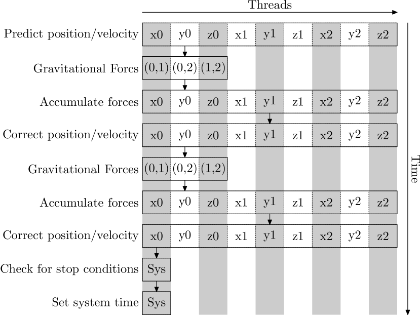
Figure 1: Illustration of effort distribution across threads with a multiprocessor for a single system with two planets using the Hermite integrator and default gravitation class. The notation x1..z2 indicates the component and body number that is being assigned as a part of current task. (i,j) pairs indicate that the interaction between bodies i and j being assigned to a thread as a part of current task. “Sys” refers to assignment of the current task to one thread to operate on the whole system. The execution changes parallelism for each substep. The columns represent the threads that are running and rows represent the tasks being scheduled. The active threads are shown in the boxes. For some steps, not all threads get assigned a task and some sit idle. Active threads from different systems are grouped into a single warp, allowing the GPU scheduler to minimize the number of idle threads.

The raw computational power of modern GPUs can result in performance being limited by memory transfer. Therefore, a general rule of thumb for optimizing GPU code is to implement parallel algorithms that hide memory latency by providing the GPU enough work to remain well-utilized for one set of calculations while waiting for data for a subsequent set of calculations.

Our original implementation of Swarm-NG (v0.1) used only one thread per system. This work model led to a simple parallelization and was quite efficient for large ensembles of small systems using the Hermite integrator. However, fully utilizing the GPU required a large ensemble of systems and that each thread use a significant amount of memory, even for the Hermite integrator. With the advent of the GF100-based Fermi GPUs, the maximum number of registers per thread was significantly reduced (i.e., from 255 to 63). While the code still worked, the code’s efficiency depended on a large number of registers. Registers spilled into GPU-device memory and overflowed the L1 cache. Initially, the performance of Swarm-NG v0.1 was reduced when using Fermi GPUs. This led us to implement highly parallelized work models. There are four different work models currently used in Swarm-NG:

• System per thread: One thread performs all computations related to one system.

• Body per thread: One thread is responsible for calculations pertaining to one body.

• Component per thread: One thread is responsible for calculations related to one coordinate component (i.e., x, y or z) of one body. Operations are carried out on the same component of multiple vectors (e.g., position, velocity and acceleration).

• Body-pair per thread: One thread is responsible for calculations related to one pair of bodies within one  $n$-body system (e.g., mutual interaction between bodies).

While the entire integration could be parallelized using the system per thread work model (as in Swarm-NG v0.1), the GPU efficiency can be significantly increased using finer-grained parallelism. Since threads within a thread block can communicate efficiently using shared memory, we can distribute the calculations for one system over multiple threads. The vast majority of calculations can be parallelized using the body per thread work model ($n$ threads per system). While this scheme provides a significant improvement over system per thread, we found that the performance could be increased further by using still finer-grained parallelism. For example, for most integrators, the majority of the code for the actual integration (i.e., updating the positions and velocities once derivatives have been computed) can be parallelized using the component per thread work model ($3\times\mbox{$n$}$ threads per system). One notable exception is the drift step of the MVS integrator that uses the body per thread work model.

The most computationally intensive portion of the integration is calculating mutual forces between each pair of bodies (specifically the reciprocal square root) in order to calculate the acceleration of each body. For sufficiently small $n$, the mutual component of the force between each body pair can be stored in shared memory, so that each force is only computed once. In this case, the body-pair per thread work model provides the finest grain parallelization ($\frac{\mbox{$n$}(\mbox{$n$}-1)}{2}$ threads per system) for calculating the distances between body pairs. The final step of accumulating the accelerations acting on a given body is to revert to the component per thread work model.

Since no single work model is optimal for all parts of the required calculations, Swarm-NG utilizes different work models for different parts of the simulation to maximize the GPU efficiency. The kernel is launched with the maximum number of threads to accommodate any of the work models. We use simple conditional C structures (if statements operating on the thread ID) to assign tasks to the appropriate worker threads and leave the extra threads idle. We issue a syncthreads() when we switch between work models to ensure correct flow of data. Figure 1 is an example of this scheme being applied to fixed time step Hermite algorithm with default gravitation implementation for a system with two planets.

We dramatically improved performance of Swarm-NG on Fermi GPUs by implementing the more fine-grained parallelization. When using the maximum number of threads per multiprocessor, the GF100-based GPUs have fewer register per thread than the GT200-based GPUs. The new work models is better suited for using fewer registers per thread and still results in higher performance than the original implementation when using GT200-based cards (for most ensemble parameters). Further, Swarm-NG’s performance is significantly improved using either GT200 or GF100-based GPUs for ensembles with fewer systems, systems with more bodies or more memory intensive integrators. We are optimistic that our current implementation will scale well on the next generation of NVIDIA GPUs (i.e., codename “Kepler”).

4.2 Gravitational force calculations

For CPU-based  $n$-body integrators, the most computationally expensive part of the integration is the force calculation, as it requires computing a square root to determine the distance between every pair of bodies. Therefore, special attention was paid to optimizing the force calculation in Swarm-NG.

For small  $n$-body systems, Swarm-NG uses the body-pair per thread work model to achieve maximum efficiency when calculating the acceleration per unit mass between each pair of bodies exactly once and in parallel.

For the Hermite integrators, we also calculate the jerk per unit mass between each pair of bodies. The results are stored in shared memory and threads within the block synchronize. Then, the work model reverts to component per thread, and each thread accumulates the one component of the accelerations (and jerks for Hermite integrators) from each of the other bodies. While the function Gravitation::sum() has four branches inside a loop, the compiler is likely to unroll the loop and optimize the branches. Further, all threads within a warp take the same branch of the remaining if statement. In this implementation each block requires storing $3\mbox{$n_{\rm systems/block}$}\times\frac{\mbox{$n$}(\mbox{$n$}-1)}{2}$ double precision values in the multiprocessor’s shared memory (twice that amount for the Hermite integrators). Therefore, this version of the force calculation algorithm imposes an upper limit on $n$. For $n$ approaching this limit, the efficiency is reduced since each multiprocessor is limited in the number of blocks that it can work with to hide memory latency.

Swarm-NG also includes an alternative Gravitation class optimized for larger $n$. This version parallelizes under the component per thread work model. Its force computation calculates each square root twice: once when calculating the acceleration of body i due to body j and once for calculating the acceleration of body j due to body i. As a result, each block stores the magnitude of the acceleration (and jerk for Hermite integrators) for only $\mbox{$n$}\times\mbox{$n_{\rm systems/block}$}$ body-pairs into shared memory at a time. Since only $\mbox{$n$}\times\mbox{$n_{\rm systems/block}$}$ (or $2\mbox{$n$}\times\mbox{$n_{\rm blocksize}$}$ for Hermite) double precision values are stored in shared memory, this algorithm can handle significantly larger $n$.

In both variants of the force calculation, the impact of the massive star (body 0) on acceleration (or jerk) is accumulated last.

4.3 Integrators

Algorithm 1 Pseudo code for the generic algorithm highlighting the components of the framework, including integrator, monitor, force calculation time step adaptation.

  $\mathbf{M}\leftarrow$ instance of monitor component for the system

  $\mathbf{G}\leftarrow$ instance of gravitation component for the system

  $\mathbf{P}\leftarrow$ instance of propagator component for the system with $\mathbf{G}$ as gravitation component

  prepare($\mathbf{P}$)

  while $state_{system}=$ active and $count_{iterations}<max_{iterations}$ do

     advance($\mathbf{P}$)

     execute($\mathbf{M}$)

     if $time_{system}>time_{destination}$ then

        $state_{system}\leftarrow$ inactive

     end if

     $count_{iterations}\leftarrow count_{iterations}+1$

  end while

  clean up($\mathbf{P}$)

Algorithm 2 Advance procedure for Hermite propagator. Note that $x^{(0)}_{b,c}$ is the initial $c$th coordinate of $b$th body. Likewise, $v^{(0)}_{b,c}$ is the initial $c$th component of velocity of $b$th body.

  $x^{(1)}_{b,c}\leftarrow x^{(0)}_{b,c}+v^{(0)}_{b,c}\Delta t+\frac{a^{(0)}_{b,c}}{2}(\Delta t)^{2}+\frac{j^{(0)}_{b,c}}{6}(\Delta t)^{3}$

  $v^{(1)}_{b,c}\leftarrow v^{(0)}_{b,c}+a^{(0)}_{b,c}\Delta t+\frac{j^{(0)}_{b,c}}{2}(\Delta t)^{2}$

  for  $k=1$ to $2$  do

     $a^{(k)}_{b,c},j^{(k)}_{b,c}\leftarrow$ calculate acceleration and jerk($\mathbf{G}$)

     $x^{(k+1)}_{b,c}\leftarrow x^{(k)}_{b,c}-\frac{3}{10}\left(a^{(0)}_{b,c}-a^{(k)}_{b,c}\right)(\Delta t)^{2}-\frac{1}{60}\left(7j^{(0)}_{b,c}+2j^{(k)}_{b,c}\right)(\Delta t)$

     $v^{(k+1)}_{b,c}\leftarrow v^{(0)}_{b,c}-\frac{1}{2}\left(a^{(0)}_{b,c}-a^{(k)}_{b,c}\right)\Delta t-\frac{1}{12}\left(5j^{(0)}_{b,c}+j^{(k)}_{b,c}\right)(\Delta t)^{2}$

  end for

  $time^{\prime}_{system}\leftarrow time_{system}+\Delta t$

Swarm-NG includes several integrators that build on the common data structures and work models described above. This framework makes it easy for a developer to implement a new integrator that takes advantage of the highly parallel GPU architecture with minimal attention to hardware details. First, we describe the common pattern for Swarm-NG integrators. Then, we discuss implementation details relevant to specific integrators.

Swarm-NG provides a generic GPU integrator class that facilitates rapid development and testing of various integration algorithms and/or parallelization schemes. The generic integrator class provides common logic, such as setting which threads are active and which are idle for various portions of the calculation, generating references and pointers to the system, logging the system state, and enforcing the stopping criteria. A simplified pseudocode is listed in Algorithm 1. A “propagator” class is responsible for advancing the system by one time step (e.g., Hermite propagator in Algorithm 2). A “monitor” class is responsible for determining when the system state should be logged and when the GPU should cease integrating a given system. The generic integrator automatically enforces a maximum number of iterations of the propagator and a maximum destination time, separate from the monitor class.

After some initial setup, the generic GPU integrator kernel initializes the monitor and propagator while providing monitor and propagator their respective parameters. Next, it enters a loop allowing for many propagator steps within a single GPU kernel call, so as to minimize overhead associated with each kernel call. For each iteration, the generic integrator calculates the maximum time step, calls the propagator’s advance() function, synchronizes threads, calls the monitor function and resynchronizes the threads. If the monitor determines that logging is needed, then the system’s current state is written to a buffer in the GPU global device memory. The system can be set inactive either by the monitor class or if the system reaches the destination time.

While the generic GPU integrator class allows for developers to focus on their algorithm with minimal attention to bookkeeping and GPU hardware, it incurs some additional overhead, and imposes some constraints on the structure. The overhead can be significant for relatively simple integrators and few-body systems (e.g., Hermite). Therefore, Swarm-NG also offers the developer the option of writing a GPU integrator kernel that bypasses the generic GPU integrator class. The developer is still able to avoid many details of GPU programming by inheriting from a GPU integrator base class and reusing data structures and programming patterns from existing integrators.

4.3.1 Hermite Integrator

The Hermite integrator closely follows the pattern of the generic GPU integrator. There are three differences. A thread loads the position and velocity of the body-component that it is assigned once prior to entering the loop over multiple integration steps, rather than loading the data at the beginning of each integration step. Since Hermite has a relatively small integration kernel, removing the additional loads improves performance. Second, the Hermite integrator has been optimized to remove syncthreads() calls that are needed in the generic GPU integrator to ensure correctness, but are not necessary for the Hermite integrator. With the reduced number of synchronization statements, the GPU has more flexibility in assigning threads to hide memory latency.

Finally, the Hermite integrator requires both the acceleration and the jerk be computed analytically. Therefore, it must use a gravitation class that computes both the acceleration and jerk. As a result, the Hermite integrator uses more shared memory per block than the Verlet, Runge-Kutta and MVS integrators, so fewer systems can be assigned to a multiprocessor simultaneously. As a result either the number of systems per block or the maximum number of blocks executing on a multiprocessor is reduced relative to an integrator which uses a Gravitation class that does not require computing the jerk.

Time Step adaptation

For adaptive time steps, the user specifies a constant step size scale ($\tau$). During each step, the simulation time is advanced by a time step ($\Delta t$) that is recalculated based on the ratio of the acceleration and the jerk for each body,

$$\Delta t=\tau\left[\sum_{i}\frac{\left|{\bf j}_{i,0}\right|^{2}}{\left|{\bf a}_{i,0}\right|^{2}}\right]^{-\frac{1}{2}},$$ (5)

where $i$ indexes a body in the system. Each acceleration and jerk component for each body is computed by the Gravitation class. These values are written to shared memory and the ratio $\left|{\bf j}_{i,0}\right|^{2}/\left|{\bf a}_{i,0}\right|^{2}$ is determined using the body per thread work model. The summation is performed using the system per thread work model and the result is distributed to all threads using shared memory.

Since the above time step algorithm uses only the values at the beginning of the time step, technically, it is not fully time-symmetric. In principle, one could ensure time symmetry by iterating until the time steps calculated using the coordinates at the beginning and end of the step are the same. To facilitate convergence, one could choose from a discrete set of time steps, e.g., $\tau\times 2^{q}$ for any integer $q$ [17]. Such a time step scheme could be valuable if the Hermite integrator were to be used for long-term integrations. However, complete time symmetry is often not essential for short-term integrations, the most common use case for the Hermite integrator.

4.3.2 Runge-Kutta Integrator

The fixed time step Runge-Kutta integrator implementation is very similar to that of the fixed time step Hermite integrator. Since Runge-Kutta uses the acceleration (and not the jerk), it uses less shared memory per system than the Hermite integrator, potentially allowing a multiprocessor to integrate more systems simultaneously. However, the Runge-Kutta integrator requires more than three times as many computations per step (i.e., six rather than three force calculations per step). Furthermore, the Runge-Kutta integrator requires much more memory for local variables than the Hermite integrator. The local variables may not fit in registers, and for practical block sizes the local variables may not even fit into the L1 cache on current Fermi GPUs. Therefore, local variables spill over into the L2 cache and perhaps global device memory. This results in significantly greater latency in accessing memory and reduces computation throughput.

Time Step Adaptation

The adaptive version of Runge-Kutta integrator uses the Cash-Karp method at the end of the step to compute the 5th order error. If the error exceeds the user spec- ified accuracy parameter error tolerance ($\epsilon$), The step is rejected, e.g, positions, velocities and time are not updated in the device memory. Instead, the next attempted time-step will use a smaller time-step.

4.3.3 MVS Integrator

The Mixed-Variable Symplectic (MVS) integrator is implemented as a propagator to be used with the generic GPU integrator. The four sub-steps that use Cartesian coordinates (both Cartesian drift sub-steps and both kick sub-steps; see §2.2.3) use the body-component per thread work model. The force calculation is implemented the same as for Runge-Kutta and uses the body-pair per thread work model for small $n$. The Keplerian drift sub-step (drifting along a Keplerian orbit; see §2.2.3) and the variable transformations are performed using the body per thread work model. Since the separation between planets does not change during Cartesian drift and kick sub-steps, we reuse the accelerations calculated after Keplerian drift substep at the beginning of the next step.

4.4 Optimizations

Coalesced Memory Access

In current CUDA architecture, the threads within a block are assembled into “warps”, a group of $n_{\rm warpsize}$ threads ($\mbox{$n_{\rm warpsize}$}=32$ on current NVIDIAGPUs) that are executed (nearly) concurrently.

Although only one warp can be executed at once, multiprocessor can schedule warps to execute in a manner that hides memory latency for load and store operations. Load/store operations can be significantly faster if threads within a warp access data in a contiguous region of memory. This is known as “coalesced” memory access.

Swarm-NG provides data structures (CoalescedStructArray and CoalescedMemberArray) that facilitate coalesced memory access and generally optimize the memory access pattern. Using these classes, accessing these arrays correctly is transparent to developers. In the data structures, systems are grouped into “chunks”. The data for the same member of a structure for all systems within a chunk is stored consecutively, so as to facilitate coalesced memory access. The number of systems in a chunk ($n_{\rm chunksize}$) must be power of 2 and can be set at compile time to a number between 1 and 32. For fully coalesced memory access, $n_{\rm chunksize}$ should be chosen in a way that $\mbox{$n_{\rm chunksize}$}\geq\mbox{$n_{\rm warpsize}$}$ and $\mbox{$n_{\rm systems/block}$}=m\times\mbox{$n_{\rm chunksize}$}$ for some integer $m$.

The non-trivial data structure minimizes the cost of load/store operations by allowing for both coalesced memory access and good cache performance (as compared to a structure of arrays indexed by the system number).

Coherent Execution

The chunk-based data structures also have implications for the organization of threads within a block. If multiple threads within a warp take different branches (e.g., an if statement or loop), then the time required is as if all threads executed every branch taken by any of the threads within the warp. Therefore, maximum efficiency is achieved when a warp is “coherent”, meaning that all threads within the warp execute the same instructions by taking the same branch of conditional statements or loops.

Within a block of threads, threads are organized into a two dimensional thread grid, where the dimensions of the outer array is the number of threads per system ($n_{\rm thread}$) and the dimension of the inner dimension is the number of systems per block. This implies that systems within a chunk that access the same structure member are accessing a continuous region of memory, allowing them to benefit from coalesced memory access. Additionally, the threads are organized so that underutilized threads are ordered consecutively, allowing the GPU to exit from the extra threads efficiently. This occurs whenever the current work model uses fewer than the total number of threads launched for the kernel (e.g., during the calculation of distances for $\mbox{$n$}\leq 6$).

Caching in Fermi architecture

A second rule of thumb for optimizing GPU code is to maximize memory throughput. In general, transfer to and from global memory is expensive due to the high memory latency ($\sim$300-1000 clock cycles if not cached). The shared memory and L1 cache have much smaller latencies (e.g., $\sim$20 clock cycles). Swarm-NG uses data structures optimized to provide for both coalesced memory access and higher spatial and temporal locality. This provides significantly better performance on an architecture where cache is present (e.g., Fermi GF100 GPUs) with minimal cost for older GPUs (e.g., GT200) that do not cache GPU memory.

GPU-optimized mathematical functions

We take advantage of the GPU hardware-optimized rsqrt(x) (reciprocal square root) function which is slightly faster than 1.0/sqrt(x). Although rsqrt(x) is not IEEE-754 complaint the deviation does not introduce significant numerical error. Similarly, the MVS integrator makes use of the combined sincos(x) function.

Aggressive loop unrolling using C++ templates

We unroll small loops (e.g., over bodies or body pairs) so as to avoid loop overhead and to provide the compiler information at compile time that allows further optimization of code flow. For some loops, we use the #pragma compiler directive to unroll loops. However, the compiler may choose to ignore this directive. On the other hand, the C++ compiler is obliged to unroll templates, guaranteeing that sequential code will be generated for loops and code flow can be optimized at compile time. Therefore, we use template meta-programming in order to generate static, optimized code for the most important loops, e.g., the loop over body pairs in the gravitation class. The static code generation gives a better performance at the cost of longer compile time and a significantly larger code size.

Data Reduction

For some applications, transferring data from the GPU memory to CPU memory can become a bottleneck. Data reduction is the strategy of choosing to download only a subset of data and/or performing post-processing on the GPU, so less data needs to be transferred to CPU, reducing CPU-GPU communication overhead.

When using the simplest syntax, Swarm-NG synchronizes the state of the ensemble between the CPU and GPU before and after each kernel call. Advanced programmers may choose to call the  $n$-body integrator kernel without invoking CPU-GPU memory transfer, provided they manage the CPU-GPU memory transfer separately. This can be useful for applications that frequently inspect the state of the systems, but do not need all data about every system. For example, when comparing model planetary systems to radial velocity observations, one only need to inspect the star’s radial velocity, rather than every component of every body. Transferring only these coordinates reduces the amount of memory transferred by more than a factor of six. Another example consists of monitoring the energy and/or angular momentum of each system. The energy and angular momentum can be calculated on the GPU, so only 1-4 values per system need to be transferred to the CPU.

Automatic selection of $n_{\rm systems/block}$ and register utilization

Our CUDA kernels utilize the maximum number of registers allowed per thread in Fermi architecture (63). Each multiprocessor has a finite size register file, so register utilization has considerable effect on overall performance of the simulation. At run-time, Swarm-NG automatically selects the block size to maximize $n_{\rm systems/block}$  considering the following three hardware resource limits: 1) the maximum number of threads allowed per multiprocessor, 2) the size of shared memory module per multiprocessor, and 3) the size of the register file per multiprocessor. The automatic selection is largely based on our performance benchmarks explained in §5.3. For a given chunk size, Swarm-NG’s performance generally increases with increasing occupancy, which is defined to be the ratio of active warps to the maximum number of warps supported on a multiprocessor. For GT200-based GPUs, Swarm-NG achieves near 25% occupancy for standard integrators. For Fermi-based GPUs, Swarm-NG achieves nearly 30% occupancy for the standard integrators. If one wants to choose the optimal values for $n_{\rm chunksize}$ and $n_{\rm systems/block}$, then we recommend performing benchmarks specifically for the problem of interest. For example, in some cases, we observe a modest performance benefit when using a smaller $n_{\rm systems/block}$, if that choice also results in an occupancy comparable to or greater than that of the maximum $n_{\rm systems/block}$. This can be due to slightly greater occupancy (due to requirement that $n_{\rm systems/block}$  is a multiple of the chunk size) or due to reducing the impact of synchronization operations.

5 Validation and Performance

In this section, we present the results of  $n$-body simulations that were designed to (a) verify that the GPU integrators in Swarm-NG are implemented correctly and to (b) measure how the performance of the integrators depends on simulation and implementation parameters. §5.1 lists the initial conditions for our tests and benchmarks, §5.2 explains how integrators are validated. §5.3 presents performance benchmarks.

5.1 Initial Conditions for Verification & Benchmarking

The range of possible initial conditions and the chaotic nature of the general  $n$-body problem make it impossible to test the integrators in all possible regimes. Since the accuracy and the limitations of the underlying integration algorithms are well-studied [17, 27, 30], Swarm-NG uses the regime of particular scientific interest to the authors: the integration of planetary systems.

Here, we consider a system with one central body, the ‘sun’, with mass $m_{0}=1$ placed at rest at the origin and the $n_{\rm pl}$‘planets’ indexed by $i=1$ with identical masses $m_{i}$ and initial conditions corresponding to a circular orbit about the origin with separation of $a_{i}:=(1+\alpha)^{i-1}$. Thus, the initial velocity is perpendicular to the position vector and has a magnitude $|v_{i}|=2\pi(\frac{m_{0}}{a_{i}^{3}})^{\frac{1}{2}}$. Unless specified otherwise, our benchmarks are based on the case $\mbox{$n$}=3$. Default values are relative planet masses comparable to Jupiter, $m_{i}=0.001$ (planet_mass parameter in the configuration file) with $\alpha=0.4$ (spacing_factor parameter). For $\mbox{$n_{\rm pl}$}=2$, these initial conditions are provably ‘Hill stable’, i.e., there will be no close approaches, and hence provide a test appropriate for both fixed and adaptive time step algorithms – and they are reasonable for $\mbox{$n_{\rm pl}$}>2$, where long-term orbital stability can not be guaranteed, even if equations of motion were integrated exactly.

5.2 Validation

5.2.1 Direct Comparison of Results

To compare two integrators using the same initial conditions, the Swarm-NG demonstrate code offers a ‘test’ mode, where a user can provide a set of initial conditions and a set of reference final conditions. This test mode allows users to test existing integrators in new regimes or to validate the new integrators. Swarm-NG performs the integration and compares the magnitude of the Cartesian position and velocities of each body (relative to the origin), as well as the final integration time. Passing the test requires that all match to within specified tolerances. The default value for position tolerance (pos_threshold), velocity tolerance (vel_threshold) and time tolerance (time_threshold) is $10^{-10}$.

First, we verified agreement of short-term simulations using a CPU-based Hermite integrator and a GPU-based Hermite integrator. Differences below the thresholds are due to hardware precision and/or rounding behavior such as our GPU implementation using the hardware-optimized rsqrt (reciprocal square-root) function rather than sqrt. Next, to verify the accuracy of the Swarm-NG integrators, rather than implementing a CPU version of each integrator, we compared their results to that of the GPU-based Hermite integrator. When comparing the results of two different integration algorithms, we use a sufficiently small time step or accuracy parameter so that the truncation error is minimized for both integrators. Since the actual systems are chaotic, we must restrict comparisons to short-term integrations. The Swarm-NG demonstration code’s default test integration duration is $10\pi$ time units (or 5 inner orbital periods) and can be overridden using the destination_time configuration parameter. All of Swarm-NG’s integrators pass these tests using the initial conditions described in §5.1 and the default integrator parameters for $\mbox{$n$}=3\ldots 6$.

5.2.2 Energy Conservation

To test the long-term stability of Swarm-NG GPU integrators, we monitored the total energy of a closed system evolving under Newtonian gravity. For an exact integrator, the system energy is preserved. The energy is given by

$$E=\sum_{i}m_{i}\frac{1}{2}\left|{\bf v}_{i}\right|^{2}-\sum_{i\neq j}\frac{Gm_{i}m_{j}}{\left|{\bf r}_{i}-\bf{r}_{j}\right|},$$ (6)

where $\bf{r}_{i}$ and $\bf{v}_{i}$ are the position and velocity vectors of the $i$th planet. We monitor $\left|\frac{\Delta E(t)}{E(0)}\right|=\left|\frac{E(t)-E(0)}{E(0)}\right|$, the fractional error in the energy of an integration as a function of the time in the simulation.

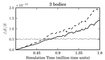
Figure 2: Energy error versus time. The three line styles correspond to simulations using the adaptive time step Hermite (solid), adaptive time step Runge-Kutta (short, but thick dashes) and MVS (dotted). Initial conditions are described in §5.1. The time step and accuracy parameters are listed in §5.2.2 and have been chosen so that the integrators have a roughly similar level of energy error after $\sim 100,000$ inner orbital periods.

We ran simulations for $2\times 10^{6}$ time units, corresponding to over 286,000 inner orbital periods. After experimenting with the time-step and accuracy parameters, we adopted $\Delta t=10^{-3}$ for Fixed time-step Hermite, $\Delta\tau=1.7\times 10^{-2}$ for Adaptive time-step Hermite, $\epsilon=5.0\times 10^{-33}$ for Adaptive time-step Runge-Kutta, and $\Delta t=10^{-2}$ for MVS. We use these values for all future benchmarks. These choices result in a very good long-term energy conservation and a roughly similar level of energy error after $\sim 100,000$ inner orbital periods, facilitating rough comparisons of the performance of different integrators over these timescales.

	Simulation Time (million time units)
Integrator	.45	.90	1.3	1.8
Hermite Adaptive	2.9	6.3	9.2	14.1
MVS	5.0	5.2	5.1	5.1
Runge-Kutta Adaptive	3.7	8.6	12.2	19.2

Table 1: Fractional energy error for selected integration algorithms. Results ($\times 10^{-11}$) are listed for $\mbox{$n$}=3$ using initial conditions as described in §5.1. The columns indicate the energy error after different integration times. Time-step parameters are listed in §5.2.2.

The growth of the fractional energy error for selected integrators is shown in Figure 2 and specific values are given in Table 1.

As expected, the Hermite and the Runge-Kutta integrators result in a slow accumulation of energy error, while the MVS integrator results in a roughly constant energy error. We verified that the Swarm-NG integrators are capable of high-precision integrations; most scientific studies use significantly larger time-steps and lower accuracy.

5.3 Performance

Machine	Cluster 1	Cluster 2	Server 1	Workstation
CUDA Device	Tesla T10	Tesla M2070	Tesla C2070	Geforce GTX480
CUDA Driver	4.2	4.2	4.2	4.2
CUDA Toolkit	4.2	4.2	4.2	4.2
Compute Capability	1.3	2.0	2.0	2.0
GPU MPs	30	14	14	15
Cores/MP	8	32	32	32
GPU Clock	1.30 GHz	1.15 GHz	1.15 GHz	1.45 GHz
GPU Memory	4GB	6GB	5GB	1.5GB
Memory Clock	800 MHz	1566 MHz	1494 MHz	1900 MHz
Shared Memory	16KB	48KB	48KB	48KB
L1 Cache Size	None	16KB	16KB	16KB
L2 Cache Size	None	768KB	768KB	768KB
Registers per MP	16384	32768	32768	32768

Table 2: Key specifications of GPUs used for performance benchmarks.

The performance of GPU integrators in Swarm-NG depends on the number of systems, $n_{\rm sys}$, the number $n$ of bodies in each system, as well as on the parameters $n_{\rm blocksize}$, $n_{\rm chunksize}$ and of course on the GPU hardware. In this section, we examine how the performance of selected GPU integrators is affected by these parameters. The results can help users optimize their choice of implementation parameters, or at least avoid particularly inefficient choices. The results also demonstrate that several of the optimizations implemented in Swarm-NG provide significant performance benefit compared to a naive GPU implementation.

Unless noted otherwise, performance benchmarks are based on integrating an ensemble of 2000 planetary systems for 1 time unit, $\mbox{$n$}=3$, $\mbox{$n_{\rm chunksize}$}=4$ and an automatically chosen number of systems per block ($n_{\rm systems/block}$); see §4.4.

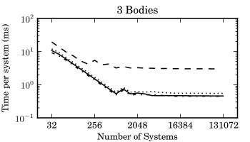
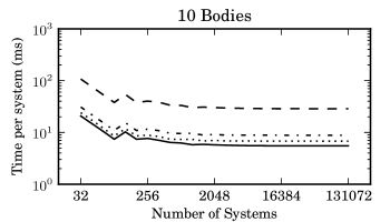
Figure 3: Wall clock time per system versus number of systems in the ensemble for the Hermite (fixed time step) integrator and the standard initial conditions and integration parameters described in §5.1 and 5.2.2. The line styles show results for different machines: Cluster 1 (dashed), Cluster 2 (dotted), Server 1 (dot-dashed), Workstation (solid).

	Machine
$n$	Cluster 1	Cluster 2	Server 1	Workstation
3	140.008	35.951	29.290	30.482
4	203.036	65.284	52.635	53.132
5	310.685	100.800	69.346	81.880
6	807.346	121.908	102.880	103.536
10	1874.480	444.202	577.674	362.020

Table 3: Performance comparison of different Machines. The numbers in table represent the time (in seconds) required to integrate the ensemble. The ensemble in this benchmark consists of 131072 systems and it was integrated for 1 time unit using the default configurations of the Hermite integrator.

Fig. 3 and Table 3 compare the performance of the Hermite and MVS integrators using three different types of GPU hardware whose specifications are given in Table 2.

Figure 3 shows that the wall clock time for integrating each system asymptotes for large $n_{\rm sys}$, as expected since both computation and memory access scale linearly. However, when there are not enough systems in the ensemble to utilize all GPU resources, the time per system significantly increases. On the other hand, the wall clock time per system is minimized when the ensemble contains enough systems to efficiently utilize the GPU’s computational resources while waiting for memory transfers. The minimum number of systems to achieve near maximum efficiency usually scales with the number of multiprocessors. On the ‘Server 1’ configuration, high efficiency is reached when the ensemble size is $\mbox{$n_{\rm sys}$}>1024$ for a 3-body system, respectively $\mbox{$n_{\rm sys}$}>128$ for a 10-body system.

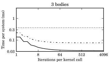
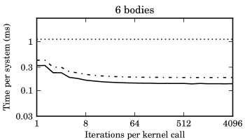
Figure 4: Wall clock time per system versus number of integrator iterations per GPU kernel call. The line styles show results for three different integrators, Hermite (solid), MVS (dotted), Runge Kutta (dotted-short dashed). Integrations were performed on Server 1 using standard initial conditions and integration parameters described in §5.1 & 5.2.2.

Next, we test our design choice of carrying out all of the computations and flow control on the GPU device. Unlike most GPU accelerated applications, Swarm-NG performs the entire  $n$-body integration on the GPU. The host program needs only set up parameters, load initial configuration onto the GPU, call the GPU-based integrator, and examine the results. Once control is transferred to GPU, the simulation runs for a configurable number of iterations, i.e., steps for Hermite or MVS integrators or trial steps for Runge-Kutta integrator.

Figure 4 shows, for Hermite and MVS integrators, that the wall clock time per system decreases as the number of iterations of the  $n$-body integrator increases. As expected, there are significant costs associated with each kernel call as demonstrated in the figure; the speed-up is $\sim~{}2.4\ldots 4$ if each kernel call performs hundreds of steps. For the Runge-Kutta integrator, the run-time is insensitive to the number of iterations. Therefore, it could have been implemented as efficiently using a separate kernel call for each step of the integrator.

While part of this overhead is the kernel launch itself and some operations are performed once per thread (e.g., calculating memory location for the system being integrated by a given thread), we posit that most of the performance decrease is due to the memory latency, i.e., the GPU not being utilized while waiting for the initial conditions to be loaded from the device global memory. Presumably, the Hermite and MVS integrators benefit from multiple steps per kernel call, since they are less memory intensive, and hence initial conditions remain in the cache between successive kernel iterations. More iterations per kernel call lead to longer kernel calls which hide the latency.

We conclude that there can be a substantial performance benefit to performing the integration fully on the GPU.

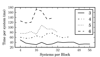
Figure 5: Wall clock time per system versus number of systems per block. The line styles show results for different number of bodies per system, as indicated in the legend. The maximum number of systems per block varies with the number of bodies per system, due to the available shared memory and the maximum number of threads per block. Integrations were performed on Server 1 using standard initial conditions and integration parameters described in §5.1 and 5.2.2.

Coalesced Memory Access

Figure 5 shows wall clock time per system varying with $n_{\rm systems/block}$. The number of systems per block must be an integer multiple of the chunk size, $n_{\rm chunksize}$. Here we set $\mbox{$n_{\rm chunksize}$}=4$, allowing for at least partially coalesced memory access and several different values of $n_{\rm systems/block}$. For $\mbox{$n$}=3$, the performance increases as $n_{\rm systems/block}$ approaches 16, likely to due the benefits of fully coalesced memory access and utilization of each warp. On the other hand, for $\mbox{$n$}=6$, the performance decreases once $\mbox{$n_{\rm blocksize}$}=16$, corresponding to the local memory within a block exceeding 16kB and potentially resulting in cache misses or limiting the number of threads that can be active at once in a multiprocessor. Thus, the variations in the time per system with $n_{\rm systems/block}$ is likely due to a combination of factors: memory caching and coalescence, and efficient utilization of threads.

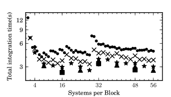
Figure 6: Wall clock time per system versus number of systems per block for $n$=3 and the fixed time-step Hermite integrator. The point styles show results for different values of the chunk size, 16 (squares), 8 (triangles), 4 (stars), 2 (x’s) and 1 (disks). Integrations were performed on Server 1 using standard initial conditions and integration parameters described in §5.1 and 5.2.2.

Figures 6 shows how the performance of the Hermite integrator with $\mbox{$n$}=3$ depends on both $n_{\rm systems/block}$ and $n_{\rm chunksize}$. The most significant performance benefits (from $\mbox{$n_{\rm systems/block}$}={1\dots 8}$) come from grouping systems into chunks which results in better memory coalescing. There is no significant gain when increasing $n_{\rm chunksize}$ from 16 to 32, indicating that a chunk size of 16 exploits the maximum amount of memory coalescing.

Since the GPU is configured to allocate 64 registers per thread, the maximum number of threads that can be launched on a multiprocessor is $\frac{32768}{64}=512$. Since the total number of threads per block is 252 for $\mbox{$n_{\rm systems/block}$}=28$ and 504 for $\mbox{$n_{\rm systems/block}$}=56$, these choices of $n_{\rm systems/block}$ result in optimal register utilization and hence best performance.

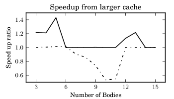
Figure 7: Ratio of wall clock time for integrations when the CUDA driver is instructed to favor (a) a configuration with 48kB L1 cache and 16kB shared memory per multiprocessor and (b) a configuration with 16kB L1 cache and 48kB shared memory per multiprocessor. Ratios greater than one indicate higher performance of configuration (a). Solid line refers to Server 1 and dotted-dashed line refers to Cluster 2. Integrations used the standard initial conditions and integration parameters described in §5.1 and 5.2.2

Fermi-based GPUs have 64kB of memory per multiprocessor that can be partitioned among shared memory and an L1 cache in two ways. This memory shares a common hardware implementation, but is accessed differently. The shared memory (either 16kB or 48kB) is user-managed, i.e., it is only accessed as instructed by the programmer. Swarm-NG uses shared memory for calculating accelerations or managing adaptive time steps, depending on the integrator and choice of gravitation class (see §4). While the programmer has no control over how the L1 cache is used, it can help hide the latency of local memory access automatically. Figure 7 compares Swarm-NG’s performance for the default configuration but with varying balance of shared memory to L1 cache.

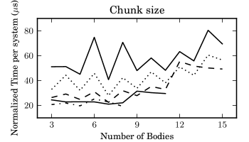
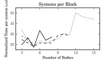
Figure 8: Normalized wall clock time per system versus number of bodies per system using the adaptive time step Hermite integrator. Here “normalized” refers to dividing the wall clock time per system by the number of body pairs. In the top panel, the line styles show results for different values of $n_{\rm chunksize}$, 1 (upper solid), 2 (dotted), 4 (dashed), 8 (lower solid) and 16 (dot-dashed). In the bottom panel, the line styles show results for different values of $n_{\rm systems/block}$, 4 (dotted), 8 (dashed), 16 (solid) and 32 (dot-dashed). Integrations were performed on Server 1 using standard initial conditions and integration parameters described in §5.1 & 5.2.2.

Figure 8 shows the wall clock time per system of the Hermite integrator normalized by the number of body pairs versus the number of massive bodies in each system. By default, values for $n_{\rm chunksize}$ and $n_{\rm systems/block}$ are chosen automatically. However, one can run benchmarks similar to ones in Figures 6 and 8 to find the optimal parameters. We find that for fixed $n$ and $n_{\rm chunksize}$, the occupancy is usually an accurate predictor of the relative performance when using two different values of $n_{\rm systems/block}$.

5.3.1 Comparison to OpenMP implementation on multi-core CPU

NBodies	CUDA	OpenMP
3	102.1	45.8
4	115.5	53.5
5	128.8	58.5
6	156.8	61.7

Table 4: Numbers of interactions per second (in millions) for different implementations of the Hermite integrator. One interaction is the force calculation between a pair of planets. Benchmarks include time spent on the integration, as well as the force calculation.

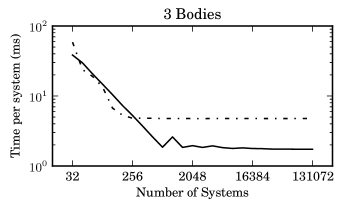
Figure 9: Comparison of GPU implementation(solid line) and CPU implementation of Hermite integrator(dotted-dashed).The integration is run for 10 time units with different number of 3-body systems. Integrations were performed on Cluster 2 using standard initial conditions and integration parameters described in §5.1 & 5.2.2.

In the beginning, we implemented a simple implementation of Hermite integrator in CPU as a reference implementation. The main purpose of the CPU implementation is to verify correctness of GPU implementation. For this reason, we tried to avoid hand optimization and complex features in CPU implementation to avoid logical errors.

However, to give a fair comparison between GPUs and multi-core CPUs, we enhanced the CPU implementation with OpenMP API to maximize performance on multi-core CPUs. We keep the code simple and rely on Intel optimizing compiler to generate fast code (same approach is used in GPU implementation with CUDA compiler).

OpenMP enhanced implementation is parallelized on a system per thread basis. The code is compiled with Intel optimizing compiler version 12.1.5 and following flags are used to optimize the code on a 6-core Intel Xeon X5675 CPU: -O3 -fast -xCORE-AVX-I -fopenmp.

Table 4 compares performance of the OpenMP implementation versus the GPU implementation in terms of interactions per second. The benchmark was generated by integrating an ensemble of 131072 systems each containing 3-bodies for 100000 steps in Hermite integrator. Figure 9 compares the wall clock time of the GPU and CPU-based Hermite integrators for 3-body systems.

6 Discussion

Swarm-NG enables fast parallel simulation of thousands of few-body systems using modern GPUs. The Swarm-NG package includes a high-level API and powerful demonstration programs, already in use for science. Code samples illustrate Swarm-NG’s modular nature and how to easily add functionality such as custom data logging, stopping conditions, user-specified force laws and even custom integrators.

Swarm-NG permits hand-optimizing modules that try to boost performance of every aspect (i.e., integration, force calculation, data logging, stopping criteria) for specific applications. We recommend these be used sparingly for two reasons. First, such optimization means writing software specific to the hardware whose architecture changes from time to time. In such case, the code need to be revised (or rewritten) for optimized performance on the new architecture – a cumbersome process as we experienced when migrating from GT200 to GF100. Second, modularity of the code is important to allow non-CUDA-savvy users to choose from a variety of integration schemes, force laws, stopping conditions and logging options. Indeed, one of the major achievements of Swarm-NG is to leverage compiler optimization and template meta-programming to achieve a highly optimized code, rather than compromising the clear high-level structure of the code.

6.1 Comparison to Odeint

The only alternative project we are aware of, that offers scientific grade integrations of ODEs on GPU, is Odeint. Odeint is a C++ framework for solving ODEs based on template meta-programming and can integrate systems using either the CPU or the GPU [1]. Support for integrating ODEs on the GPU is provided via Thrust, a template library for very high-level parallel programming on GPUs and multi-core CPUs (see Ch. 26 of [15]). Early in the development, we envisioned a design similar to Odeint. However, we found that such generality came at a significant performance loss. For example, Swarm-NG’s performance has been significantly improved by careful layout of data. While code parallelized by Thrust can often results in coalesced memory access, improving cache performance through data locality (see §4.4) with Thrust would be quite difficult to achieve. As another example, Thrust does not allow users to take advantage of shared memory. For systems with small $n$, the use of shared memory reduces the number of square root calculations in the force calculation step by a factor of 6, compared to Odeint with Thrust. So, while very-high-level frameworks like Odeint and Thrust are excellent for rapid code development, common applications such as  $n$-body integration can benefit greatly from being implemented directly in CUDA.

6.2 Applications

Few-body integration is a ubiquitous tool in computational astrophysics and planetary science. Swarm-NG has already proven useful for several applications related to the evolution of planetary systems.

One class of applications is related to studying planet formation in a general sense, such as characterizing the stability of tightly-packed planetary systems (Bédorf et al. in prep.) or investigating the effects of stellar flybys on planetary systems [4]. Swarm-NG makes it practical to integrate a large number of hypothetical planetary systems, required to characterize how the orbital evolution depends on the initial conditions. Another class of applications involves studying actual planetary systems. For example, by assuming that billion year-old planetary systems are long-term stable, Swarm-NG has placed limits on the masses and eccentricities of planetary systems discovered by NASA’s Kepler mission [7, 13]. A sort of hybrid scenario involves integrating a large ensemble of planetary systems similar to an actual planetary system, but varying one or two of the initial conditions to determine how close the actual system is to an unstable region of phase space. NASA’s Kepler mission recently discovered the first planetary systems containing a planet orbiting not one, but a pair of main-sequence stars. Swarm-NG was used to show that a modest reduction in the semi-major axis of the planet would render these systems unstable [7, 28].

One key application of Swarm-NG is for the self-consistent analysis of astronomical observations of extrasolar planetary systems. Most confirmed extrasolar planets have been discovered by measuring a pattern of changes in the velocity of the host star via Doppler spectroscopy. A Bayesian framework provides the basis for inferring physical parameters (and their uncertainties) from astronomical observations. Markov chain Monte Carlo (MCMC) methods are now routinely used for rigorous analyses of single planet systems [10]. The analysis of systems with multiple planets is much more computationally demanding, both because of the higher-dimensional parameter space and the need to perform an  $n$-body integration for each model evaluation. For some multiple-planet systems, the orbital motion can be well-approximated as the linear superposition of the motion of each star-planet pair [11]. However, for other systems, mutual planetary interactions produce significant observable consequences even on observable timescales, so direct  $n$-body integrations are necessary to properly interpret the observations [16, 19, 20, 21, 25, 31]. While standard MCMC algorithms are serial in nature, population-based MCMC algorithms can take advantage of GPUs ability to integrate many planetary systems in parallel. In particular, the Differential Evolution Markov chain Monte Carlo (DEMCMC) algorithm [5] is well suited to GPUs and often more efficient than a standard MCMC algorithm even when executed on a single CPU. E.B.F. has developed a DEMCMC code for the self-consistent analysis of Doppler observations of multiple planet systems. This code has already been applied to several planetary systems [16] (Wang et al., submitted to ApJ; Lee et al., in prep.; Nelson et al., in prep.). The  $n$-body integrations can be performed using either OpenMP or a GPU, using the Swarm-NG library. In the case of the 55 Cnc planetary system with 5 planets, the DEMCMC simulations required roughly three weeks, even using a Tesla C2070 GPU. Thus, the self-consistent Bayesian analysis of this system was simply not practical prior to Swarm-NG.

The other common method for discovering extrasolar planets involves measuring the apparent brightness of the host star decrease when a planet passes in front of the star. As for systems discovered by the Doppler method, Bayesian analysis of a single planet system is relatively straight forward using either a standard MCMC [29] or DEMCMC algorithm [9]. Recently, NASA’s Kepler mission has discovered hundreds of systems with multiple transiting planets. Indeed, some of the most interesting systems contain multiple closely-spaced planets that demand direct  $n$-body integration to model properly. An analysis package combining direct  $n$-body integration and the DEMCMC algorithm was implemented using MPI and a cluster of CPUs. While this code has been applied to several systems [7, 8, 28], even a two planet system can require tens of thousands of CPU hours. As the Kepler mission is continuing to return data and uncover additional planets, the computational requirements for self-consistent Bayesian analysis of Kepler data will become even more challenging. Therefore, we plan to develop a GPU-based code for performing DEMCMC analyses of Kepler observations, including direct  $n$-body integrations performed on the GPU via Swarm-NG.

While Swarm-NG was developed with a focus on planetary systems, it can be readily applied to variety of other problems, such as a system of moons orbiting a planet, scattering of multiple star systems, or even a swarm of stars orbiting a black hole.

References

- Ahnert and Mulansky [2011] Ahnert, K., Mulansky, M., 2011. Odeint - Solving ordinary differential equations in C++. CoRR abs/1110.3397.
- Bédorf et al. [2012] Bédorf, J., Gaburov, E., Portegies Zwart, S.F., 2012. A sparse octree gravitational N-body code that runs entirely on the GPU processor. Journal of Computational Physics 231, 2825–2839. 1106.1900.
- Belleman et al. [2008] Belleman, R.G., Bédorf, J., Portegies Zwart, S.F., 2008. High performance direct gravitational N-body simulations on graphics processing units II: An implementation in CUDA. New Astronomy 13, 103–112. 0707.0438.
- Boley et al. [2012] Boley, A.C., Payne, M.J., Ford, E.B., 2012. Interactions Between Moderate- and Long-Period Giant Planets: Scattering Experiments for Systems in Isolation and with Stellar Flybys. ArXiv e-prints 1204.5187.
- ter Braak [2006] ter Braak, C., 2006. A markov chain monte carlo version of the genetic algorithm differential evolution: easy bayesian computing for real parameter spaces. Statistics and Computing 16, 239–249.
- Capuzzo-Dolcetta et al. [2011] Capuzzo-Dolcetta, R., Mastrobuono-Battisti, A., Maschietti, D., 2011. NBSymple, a double parallel, symplectic N-body code running on graphic processing units. New Astronomy 16, 284–295.
- Carter et al. [2012] Carter, J.A., Agol, E., Chaplin, W.J., Basu, S., Bedding, T.R., Buchhave, L.A., Christensen-Dalsgaard, J., Deck, K.M., Elsworth, Y., Fabrycky, D.C., Ford, E.B., Fortney, J.J., Hale, S.J., Handberg, R., Hekker, S., Holman, M.J., Huber, D., Karoff, C., Kawaler, S.D., Kjeldsen, H., Lissauer, J.J., Lopez, E.D., Lund, M.N., Lundkvist, M., Metcalfe, T.S., Miglio, A., Rogers, L.A., Stello, D., Borucki, W.J., Bryson, S., Christiansen, J.L., Cochran, W.D., Geary, J.C., Gilliland, R.L., Haas, M.R., Hall, J., Howard, A.W., Jenkins, J.M., Klaus, T., Koch, D.G., Latham, D.W., MacQueen, P.J., Sasselov, D., Steffen, J.H., Twicken, J.D., Winn, J.N., 2012. Kepler-36: A Pair of Planets with Neighboring Orbits and Dissimilar Densities. ArXiv e-prints 1206.4718.
- Carter et al. [2011] Carter, J.A., Fabrycky, D.C., Ragozzine, D., Holman, M.J., Quinn, S.N., Latham, D.W., Buchhave, L.A., Van Cleve, J., Cochran, W.D., Cote, M.T., Endl, M., Ford, E.B., Haas, M.R., Jenkins, J.M., Koch, D.G., Li, J., Lissauer, J.J., MacQueen, P.J., Middour, C.K., Orosz, J.A., Rowe, J.F., Steffen, J.H., Welsh, W.F., 2011. KOI-126: A Triply Eclipsing Hierarchical Triple with Two Low-Mass Stars. Science 331, 562–. 1102.0562.
- Eastman et al. [2012] Eastman, J., Gaudi, B.S., Agol, E., 2012. EXOFAST: A fast exoplanetary fitting suite in IDL. ArXiv e-prints 1206.5798.
- Ford [2005] Ford, E.B., 2005. Quantifying the Uncertainty in the Orbits of Extrasolar Planets. AJ 129, 1706–1717. arXiv:astro-ph/0305441.
- Ford [2006] Ford, E.B., 2006. Improving the Efficiency of Markov Chain Monte Carlo for Analyzing the Orbits of Extrasolar Planets. ApJ 642, 505–522. arXiv:astro-ph/0512634.
- Ford [2009] Ford, E.B., 2009. Parallel algorithm for solving Kepler’s equation on Graphics Processing Units: Application to analysis of Doppler exoplanet searches. New Astronomy 14, 406–412. 0812.2976.
- Fressin et al. [2012] Fressin, F., Torres, G., Rowe, J.F., Charbonneau, D., Rogers, L.A., Ballard, S., Batalha, N.M., Borucki, W.J., Bryson, S.T., Buchhave, L.A., Ciardi, D.R., Désert, J.M., Dressing, C.D., Fabrycky, D.C., Ford, E.B., Gautier, III, T.N., Henze, C.E., Holman, M.J., Howard, A., Howell, S.B., Jenkins, J.M., Koch, D.G., Latham, D.W., Lissauer, J.J., Marcy, G.W., Quinn, S.N., Ragozzine, D., Sasselov, D.D., Seager, S., Barclay, T., Mullally, F., Seader, S.E., Still, M., Twicken, J.D., Thompson, S.E., Uddin, K., 2012. Two Earth-sized planets orbiting Kepler-20. Nat 482, 195–198. 1112.4550.
- Gaburov et al. [2009] Gaburov, E., Harfst, S., Portegies Zwart, S.F., 2009. SAPPORO: A way to turn your graphics cards into a GRAPE-6. CoRR abs/0902.4.
- Hwu [2011] Hwu, W.m.W., 2011. GPU Computing Gems Emerald Edition. Morgan Kaufmann Publishers Inc., San Francisco, CA, USA. 1st edition.
- Johnson et al. [2011] Johnson, J.A., Payne, M., Howard, A.W., Clubb, K.I., Ford, E.B., Bowler, B.P., Henry, G.W., Fischer, D.A., Marcy, G.W., Brewer, J.M., Schwab, C., Reffert, S., Lowe, T.B., 2011. Retired A Stars and Their Companions. VI. A Pair of Interacting Exoplanet Pairs Around the Subgiants 24 Sextanis and HD 200964. AJ 141, 16. 1007.4552.
- Kokubo et al. [1998] Kokubo, E., Yoshinaga, K., Makino, J., 1998. On a time-symmetric Hermite integrator for planetary N-body simulation. Monthly Notices of the Royal Astronomical Society 297, 1067–1072.
- Konstantinidis and Kokkotas [2010] Konstantinidis, S., Kokkotas, K.D., 2010. MYRIAD: a new N -body code for simulations of star clusters. Astronomy & Astrophysics 522, A70. 1006.3326.
- Laughlin and Chambers [2001] Laughlin, G., Chambers, J.E., 2001. Short-Term Dynamical Interactions among Extrasolar Planets. ApJL 551, L109–L113. arXiv:astro-ph/0101423.
- Lee et al. [2006] Lee, M.H., Butler, R.P., Fischer, D.A., Marcy, G.W., Vogt, S.S., 2006. On the 2:1 Orbital Resonance in the HD 82943 Planetary System. ApJ 641, 1178–1187. arXiv:astro-ph/0512551.
- Marcy et al. [2001] Marcy, G.W., Butler, R.P., Fischer, D., Vogt, S.S., Lissauer, J.J., Rivera, E.J., 2001. A Pair of Resonant Planets Orbiting GJ 876. ApJ 556, 296–301.
- Murray and Dermott [2000] Murray, C.D., Dermott, S.F., 2000. Solar System Dynamics. Cambridge University Press.
- Nguyen [2007] Nguyen, H., 2007. GPU Gem 3. Addison-Wesley Professional.
- Nitadori and Aarseth [2012] Nitadori, K., Aarseth, S.J., 2012. Accelerating NBODY6 with Graphics Processing Units. Monthly Notices of the Royal Astronomical Society 7, 8. 1205.1222.
- Payne and Ford [2011] Payne, M.J., Ford, E.B., 2011. An Analysis of Jitter and Transit Timing Variations in the HAT-P-13 System. ApJ 729, 98. 1103.0199.
- Portegies Zwart et al. [2007] Portegies Zwart, S.F., Belleman, R., Geldof, P., 2007. High Performance Direct Gravitational N-body Simulations on Graphics Processing Units 0702135.
- Press et al. [1992] Press, W.H., Teukolsky, S.A., Vetterling, W.T., Flannery, B.P., 1992. Numerical recipes in C (2nd ed.): the art of scientific computing. Cambridge University Press, New York, NY, USA.
- Welsh et al. [2012] Welsh, W.F., Orosz, J.A., Carter, J.A., Fabrycky, D.C., Ford, E.B., Lissauer, J.J., Prša, A., Quinn, S.N., Ragozzine, D., Short, D.R., Torres, G., Winn, J.N., Doyle, L.R., Barclay, T., Batalha, N., Bloemen, S., Brugamyer, E., Buchhave, L.A., Caldwell, C., Caldwell, D.A., Christiansen, J.L., Ciardi, D.R., Cochran, W.D., Endl, M., Fortney, J.J., Gautier, III, T.N., Gilliland, R.L., Haas, M.R., Hall, J.R., Holman, M.J., Howard, A.W., Howell, S.B., Isaacson, H., Jenkins, J.M., Klaus, T.C., Latham, D.W., Li, J., Marcy, G.W., Mazeh, T., Quintana, E.V., Robertson, P., Shporer, A., Steffen, J.H., Windmiller, G., Koch, D.G., Borucki, W.J., 2012. Transiting circumbinary planets Kepler-34 b and Kepler-35 b. Nat 481, 475–479. 1204.3955.
- Winn [2010] Winn, J.N., 2010. Exoplanet Transits and Occultations. pp. 55–77.
- Wisdom and Holman [1991] Wisdom, J., Holman, M., 1991. Symplectic maps for the n-body problem. The Astronomical Journal 102, 1528.
- Wright et al. [2011] Wright, J.T., Veras, D., Ford, E.B., Johnson, J.A., Marcy, G.W., Howard, A.W., Isaacson, H., Fischer, D.A., Spronck, J., Anderson, J., Valenti, J., 2011. The California Planet Survey. III. A Possible 2:1 Resonance in the Exoplanetary Triple System HD 37124. ApJ 730, 93. 1101.1097.