High Performance Direct Gravitational N-body Simulations on Graphics Processing Units
II: An implementation in CUDA

Abstract

We present the results of gravitational direct $N$-body simulations using the Graphics Processing Unit (GPU) on a commercial NVIDIA GeForce 8800GTX designed for gaming computers. The force evaluation of the $N$-body problem is implemented in “Compute Unified Device Architecture” (CUDA) using the GPU to speed-up the calculations. We tested the implementation on three different $N$-body codes: two direct $N$-body integration codes, using the 4th order predictor-corrector Hermite integrator with block time-steps, and one Barnes-Hut treecode, which uses a 2nd order leapfrog integration scheme. The integration of the equations of motions for all codes is performed on the host CPU.

We find that for $N>512$ particles the GPU outperforms the GRAPE-6Af, if some softening in the force calculation is accepted. Without softening and for very small integration time steps the GRAPE still outperforms the GPU. We conclude that modern GPUs offer an attractive alternative to GRAPE-6Af special purpose hardware. Using the same time-step criterion, the total energy of the $N$-body system was conserved better than to one in $10^{6}$ on the GPU, only about an order of magnitude worse than obtained with GRAPE-6Af. For $N\ {\raise-2.15277pt\hbox{$\buildrel>\over{\sim}$}}\ 10^{5}$ the 8800GTX outperforms the host CPU by a factor of about 100 and runs at about the same speed as the GRAPE-6Af.

1 Introduction

The introduction of multiple processing cores in one chip allows microprocessor manufacturers to improve the performance of CPUs while the clock rate stays the same. This multi-core principle is not new. Over the last decade, a similar approach has been taken by manufacturers of graphics processing units (GPU) under the influence of the gaming industry to deliver increasingly detailed and responsive computer games. As a result of this, the GPU underwent a dramatic increase in performance; a doubling in performance over a period of 9 months, instead of 18 months for CPUs (NVIDIA, 2007; Moore, 1965).

In terms of raw performance, today’s GPUs outperform conventional CPUs. For example, the NVIDIA GeForce 8800GTX has a performance of about 350 GFLOP/s (see § 4). However, harvesting this computing power is not trivial as GPUs are designed and optimized for graphics operations. Over the last 7 years GPUs have evolved from fixed function hardware for the support of primitive graphical operations to programmable processors that outperform conventional CPUs, in particular for vectorizable parallel operations. Today’s GPUs contain many multiple smaller processors called stream processors (Owens, 2005), that are specialized in processing large amounts of data in a streaming and parallel fashion. It is because of these developments that more and more people use the GPU for wider purposes than just for graphics (Fernando, 2004; Pharr & Fernando, 2005; Buck et al., 2004).

Initially, the programming of GPUs was done in assembly language and required a very specific knowledge of the hardware. Newer generations of GPUs offered more possibilities for the programmer and with this came the need for high-level programming languages. With the introduction of shading languages like Cg (Mark et al., 2003) and GLSL (Kessenich et al., 2007), the programmer could focus on the problem at hand.

Around this time, the performance of the GPU attracted the attention of researchers with an interest in the use of the GPU as a high-performance coprocessor. First implementations mapped their problems into a graphics problem where data is represented as coloured pixels stored in textures. Shading programs were then used to perform computations on the data. Although not every problem is easily represented as a graphics problem, the use of the GPU was demonstrated in many scientific areas, including but not limiting to PDE solvers, ray tracing, image segmentation and gravitational simulations (Owens et al., 2007).

One downside of the GPU is that the current generation only supports single precision (32-bit) floating point arithmetic. This limits their use to applications for which single precision is sufficient. In the release notes of Compute Unified Device Architecture (CUDA) version 0.8, NVIDIA announced that GPUs supporting 64-bit double precision floating point arithmetic will become available in late 2007 (NVIDIA, 2007).

In this second paper on high performance $N$-body simulations using GPUs, we present an implantation using CUDA, and apply the implementation to solve gravitational $N$-body systems using direct integration as well as using a Barnes-Hut tree code (Barnes & Hut, 1986). In our previous paper (Portegies Zwart et al., 2007) (which we from now on will call “paper I”) we presented an implementation in Cg, and showed that for $N\ {\raise-2.15277pt\hbox{$\buildrel>\over{\sim}$}}\ 10^{4}$ the GPU outperforms the CPU by about a order of magnitude.

The implementation described in this paper was born while we were drinking beer (whereas Hamada & Iitaka (2007) drank tea), so we have named our implementation kirin after a Japanese brand of beer. In § 2 we cover the background of the $N$-body problem and previous implementations. Section § 3 describes our implementation. The last two sections, § 4 and § 5 cover the results and the discussion.

2 Background

The $N$-body gravitational algorithm is based on the force equation as discovered by Newton. The equation calculates the force between two particles in space:

$${\bf F}_{i}\equiv m_{i}{\bf a}_{i}=m_{i}G\sum^{N}_{j=1,j\neq i}m_{j}{{\bf r}_{i}-{\bf r}_{j}\over|{\bf r}_{i}-{\bf r}_{j}|^{3}}.$$ (1)

Here $G$ is the Newton constant, $m_{i}$ is the mass of star $i$ and ${\bf r}_{i}$ is the position of star $i$. The total force ${\bf F}_{i}$ (or the acceleration ${\bf a}_{i}$) that is exercised on particle $i$ is the summation over the forces between $i$ and all $N$ particles.

In order to determine the total force on each particle within an $N$-body system, the force exerted by all $N$ particles has to be calculated. Calculating the force of all particles in the $N$-body system requires ${1\over 2}N(N-1)$ force calculations. This O($N^{2}$) part of the algorithm is the computationally most expensive part. The calculation of the force exerted on each particle is independent of the calculations performed for other particles. This makes the calculation of the forces for all particles parallelizable.

A breakthrough in direct-summation $N$-body simulations came in the late 1990s with the development of the GRAPE series of special-purpose computers (Makino & Taiji, 1998), which achieves spectacular speedups by implementing the entire force calculation in hardware and placing many force pipelines on a single chip. The latest special purpose computer for gravitational $N$-body simulations, GRAPE6, performs at a peak speed of about 64 TFLOP/s (Makino, 2001). The GRAPE opened the way for the simulation of large star clusters. In simulation software such as starlab (Portegies Zwart et al., 2001), for example, the GRAPE is used as a coprocessor for the force calculations. In this paper we compare our results with the GRAPE-6Af, which is a smaller commercial version of the GRAPE6. The GRAPE-6Af contains four GRAPE6 chips that are mounted on a PCI-card. The performance of the GRAPE-6Af is 123 GFLOP/s and the memory has a maximum capacity of 131072 particles.

Graphics Processing Units (GPU) can be used as an alternative coprocessor to the GRAPE in $N$-body calculations. GPUs contain many processing units that each perform the same series of operations on different streams of input data, a technique which is better known as Single Instruction Multiple Data (SIMD). The first gravitational $N$-body simulations on GPUs were presented by Nyland L. (2004) and later their implementation was improved by Mark Harris (Harris, 2005). Their implementation only performs force calculations using a simplified shared time-step algorithm. A Cg implementation that performs force, jerk and potential calculations on a GPU through a block time-step algorithm is described in paper I. There we concluded that for large $N$ the GPU offers an attractive alternative for the GRAPE-6Af because of its wide availability, low price and high reliability.

Recently the use of GPUs has attracted a lot of attention for performing direct $N$-body force calculations (Hamada & Iitaka, 2007; Elsen et al., 2007). Elsen et al. (2007) uses AMD/ATI hardware, whereas Hamada & Iitaka (2007) uses NVIDIA GPU cards. The latter also use CUDA to implement the force calculations, achieving an even higher performance than presented in paper I. Hamada & Iitaka (2007) tested the code only on an implementation using shared time-steps and with softening. We present a library, implemented in CUDA, that uses similar principles as the implementation by (Hamada & Iitaka, 2007). Our library (called kirin) can be used for direct $N$-body simulations as well as for treecodes, it can be run with shared-time steps or with block time-steps and allows non-softened potentials.

The CUDA framework exposes the GPU as a parallel data streaming processor that consists of many processing units. Compared with previous programming interfaces such as Cg, CUDA provides more flexibility to efficiently map a computing problem onto the hardware architecture. CUDA applications consist of two parts. The first executes on the GPU and is called a “kernel”. Kernels are implemented in the CUDA programming language, which is basically the “C” programming language extended with a number of keywords. The other part executes on the host CPU and provides control over data transfers between CPU and GPU and the execution of kernels.

A kernel program is run by multiple threads that run on the GPU. We call a group of threads a bundle. Threads contained in the same bundle communicate with each other using shared memory and cannot communicate with threads in another bundle. Calculations on the GPU are started by specifying the number of bundles to execute and the number of threads that each bundle contains. The total number of threads is the product of the two.

The NVIDIA GeForce 8800GTX hardware architecture defines a hierarchical memory structure where each level has a different size, access restrictions and access speed. In general, accessing the largest type of memory is flexible but slow, while accessing the smallest type of memory is restrictive but fast. This memory structure is directly exposed by the CUDA programming framework. The challenge in mapping a computing problem efficiently on a GPU through CUDA is to store frequently used data items in the fastest memory, while keeping as much of the data on the device as possible.

Current GPUs support 32-bit IEEE floating point numbers, which is below the average general purpose processor, but for many applications it turns out that the higher (double) precision can be emulated at some cost or is not crucial. The relatively low accuracy of the GPU hinders high precision direct $N$-body integrations, but is very suitable for methods which intrinsically have a lower precision, such as the Barnes-Hut treecode. We therefore tested our library for GPU-enabled $N$-body simulations on a direct integration method (§ 4.1 and § 4.2) as well as using a treecode (§ 4.3).

3 Implementation

The $N$-body scheme used in our implementation is described by Makino & Aarseth (1992). The integration scheme consists of three parts: a predictor step that predicts a particle’s position and velocity; a Hermite integrator to advance the position and velocity to the new time-step and a corrector step that corrects the predicted position and velocity using the results of the integrator. The acceleration, its time derivative (jerk) and potential are computed by direct summation.

3.1 Decomposition over CPU and GPU

In our implementation, the calculation of force, potential and jerk is performed on the GPU. The predictor and corrector steps are performed on the CPU. Our algorithm uses a block time-step scheme that only integrates subsets (blocks) of particles that need to be updated (McMillan & Aarseth, 1993).

The decomposition of this scheme over a CPU and GPU was done for two reasons. First; the prediction and correction steps are more sensitive to round-off errors and are therefore best performed using the CPU’s 64-bit floating point representation. Second; production quality software such as starlab (Portegies Zwart et al., 2001) uses a similar decomposition, but then in combination with the GRAPE coprocessor. We opted for a similar decomposition as used for the GRAPE to allow astronomical production software to link in our GPU implementation as a library.

Our implementation requires that particle data is communicated between the CPU and the GPU at each block time-step. This is accomplished through a number of memory copies where the CPU sends particle position, velocity and mass to the GPU. The results computed by the GPU (acceleration, jerk and potential) are retrieved by the CPU. For the GPU library the prediction is performed on the CPU after which all particles are copied to the GPU. The GRAPE only has to send the updated particles and performs the prediction on the GRAPE hardware itself. This results in an overall lower performance for the GPU than for the GRAPE, because the overhead of the memory copies increases much more for the GPU than for the GRAPE.

The input and output variables exchanged with the GPU program are the following:

• Input: mass ($N$), position ($3N$) and velocity ($3N$),

• Output: acceleration ($3N$), jerk ($3N$) and potential ($N$)

All values are represented by single precision (32-bit) floating point values, which is the most precise representation offered by current generation GPUs. This adds up to 14 floats or 56 bytes per particle which results in a total capacity of approximately 14 million particles for the 768MB on-board memory available on the GeForce 8800GTX. This is a substantial increase in capacity compared to the GRAPE-6Af’s maximum capacity of 131072 particles. This is also an improvement over the 9 million particles that could be stored with the earlier Cg implementation in paper I. A restriction imposed by Cg that does not allow memory areas to be readable and writable at the same time forced this implementation to use a double-buffering scheme. This restriction does not exist in the CUDA implementation described here.

The fundamental structure of our CUDA implementation aims at exploiting the available computing resources as much as possible. The challenge in mapping our $N$-body problem on a GPU through CUDA is to annihilate wait states due to slow memory accesses while keeping the threads executing on the GPU occupied.

Global memory access is slow (400 to 600 clock cycles) while shared memory access is fast (4 clock cycles) but has a limited capacity. We therefore pre-cache particles into shared memory up to its maximum capacity before the calculation of forces. The input data is split in smaller parts that are each pre-cached and processed in consecutive bursts.

The integration of one block time-step is initialised by assigning a thread to each of the particles in a block. Each thread then goes through the following steps:

1. Each thread in the bundle caches one particle from global memory into the shared memory. The total number of read particles is therefor equal to the number of threads contained in a bundle.

2. The force, potential and jerk for the thread are calculated using the particles that are cached in shared memory. The thread then sums the partial results into temporary variables which are stored in a register.

3. Steps (1) and (2) are repeated until all $N$ particles have been read.

4. When all parts are processed, the self interaction of the potential value is removed, the results are saved in global memory and the thread exits.

Note that the total number of calculations performed by the GPU with this scheme is $N^{2}$. Although it is possible to determine the force using ${1\over 2}N(N-1)$ calculations, this would require internal communication and synchronization. This added communication is costly in a GPU and would result in lower performance even though less work is done.

The method of giving each thread its own specific data and allowing data that is needed by multiple threads to be stored in shared memory is generally accepted as the best method to reduce memory latency when using CUDA capable GPUs. Shared memory significantly reduces the wait time that occurs while using global memory. This speeds-up the algorithm by reducing the number of global memory accesses.

In our implementation the number of bundles that is started depends on the number of particles in the current time-step block. Each bundle in our implementation contains 128 threads. Therefore the force, jerk and potential of 128 particles is calculated in parallel. In comparison; the GRAPE-6Af does the same but for 48 particles. The number of bundles that are started is equal to the number of particles in the time-step block divided by 128. This reduces the number of global memory accesses by a factor 128. Our implementation uses the thread scheduler to swap in threads that have already loaded their data while threads that are waiting on memory loads are swapped out. Once all threads have loaded the particle data from global memory into the shared memory space of the bundle, all threads in the same bundle can operate on that data. Through this strategy, the latency incurred by global memory accesses is hidden, which speeds up the algorithm considerably. In Fig. 1 we illustrate the memory configuration used in our implementation.

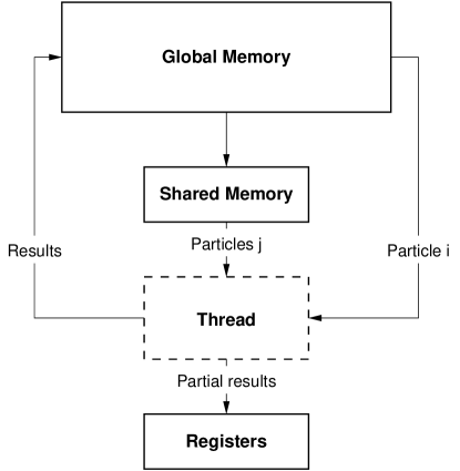
Figure 1: The memory access strategy used in our implementation to compute the force for particle $i$. Data for particle $i$ is taken directly from global memory. Each kernel copies data for particle $j$ from (slow) global memory into (fast) shared memory in parts and performs the calculations on particle $j$. This is repeated for all particles. Intermediate results are stored in registers.

3.2 Optimizing GPU utilization

The implementation described in § 3.1 has the disadvantage that it does not utilize all processors in the GPU when the number of particles in a block time-step is smaller than 4096. This number is derived as follows: To make full use of all 16 multiprocessors in the GPU it is necessary to start at least 16 bundles. Moreover, threads in a bundle that are waiting for data from global memory will be swapped out in favour of bundles for which the data is ready and can be processed, which brings the total number of bundles to 32. With our implementation, where we start 128 threads for each bundle, we must have at least $32\times 128=4096$ particles in the block time-step to fully utilize all 16 multiprocessors.

To fully utilize the GPU for any number of particles in the block time-step we have altered the implementation in such a way that it splits the calculations in several parts and then combines the partial results on the host. This is done when there are less then 4096 particles in the block time-step.

The implementation divides the total number of particles in several parts that are processed sequentially. Each part contains 128 particles, equal to the number of threads per bundle. One by one the threads in each bundle load a particle $i$ from global memory and then process the particles $j$ that have been loaded in shared memory. When we have less than 4096 particles in the block time-step, the parts that have to be processed are evenly distributed, as much as possible, over multiple bundles. Each bundle calculates a partial force between its particle $i$ and the particles $j$ in the part(s) that have been loaded from global memory. The partial results are then saved in global memory. This strategy assures that all multiprocessors in the GPU are fully utilized. As threads in different blocks cannot communicate it is not possible to aggregate partial results from finished blocks. Therefore the partial results are saved in global memory and subsequently combined on the host CPU. The host CPU loads the partial results from the GPU and then adds the partial results together.

3.3 Mimicking the GRAPE6 library

We have designed a library around our GPU based $N$-body code that mimicks the standard GRAPE6 library. This allows existing applications that are linked to the GRAPE6 library to be used with kirin with minimal changes. Additional requirements are that the CUDA run-time libraries are installed on the system and that a graphics card capable of running CUDA applications is installed in the system. Appendix A shows a list of functions that have a GPU equivalent. GRAPE6 functions that do not require a GPU equivalent are implemented as dummy functions.

3.3.1 Kernel changes

In addition to force, jerk and potential the GRAPE hardware also calculates the nearest neighbour of every particle that is being updated, and the GRAPE has the ability to perform calculations without softening. The softening parameter $\epsilon$, introduced by Aarseth (1963), prevents very small integration steps when particles reside very close to each other. The GPU code has to be adjusted to calculate the nearest neighbour and to handle simulations without softening.

Nearest neighbours are determined by comparing the distance between each particle and all other particles in the data set. This is done as part of the force calculation; a comparison is added with each force calculation to maintain the particle with the minimum distance. When the force calculation is complete, the index to the nearest neighbour is saved in global memory, together with the force, jerk and potential results.

The distance $r_{ij}$ between two particles $i$ and $j$ can be zero either when $i=j$ or when the distance between two particles cannot be represented within the limited precision of a single precision floating point number. This results in a division by zero in the force equation. The softening is added to the distance and has the effect that the distance between two particles can never be zero. For zero softening the resulting division by zero is circumvented by an additional check in the inner loop of the GPU program.

Adding each of these two comparisons results in lower performance: one extra comparison results in a performance drop of roughly 10%. This is mainly caused by the underlying SIMD architecture that enforces that when two threads take different branches, one has to wait until the branching thread reaches the same point in the program as the other. In Appendix A we present a list of the implemented kirin library functions.

4 Results

The simulations for the direct integration are run over 0.5 $N$-body time units (Heggie & Mathieu, 1986), but the measurements are from $t=0.25$ to $t=0.5$ to minimize the effect of initialization on the measurements. The simulations for the treecode are run over 1 $N$-body time unit, with the time measurements for $t=0$ to $t=1$. The host hardware we used are Hewlett-Packard xw8200 workstations with two Intel Xeon CPUs running at 3.4 GHz. These machines either had an NVIDIA GeForce 8800GTX graphics card in the PCI Express ($16\times$) bus or a GRAPE-6Af. The GRAPE and Cg machines ran a Linux SMP kernel version 2.6.16, Cg version 1.4 and graphics card driver 1.0-9746. The kirin measurements were performed with Linux SMP kernel version 2.6.18, CUDA Toolkit version 0.8 and graphics card driver 1.0-9751.

We compare the energy of the simulated system at the start and end of the simulation. The total energy $E$ within an isolated system must remain constant. We determine the relative error ${\triangle E/E}$ using the following equation:

$${\triangle E/E}={E_{start}-E_{end}\over{E_{start}}}.$$ (2)

4.1 Direct $N$-body integration in a test environment

In Table 1 we compare the performance of our CUDA implementation with the GRAPE-6Af hardware and the Cg implementation described in paper I. Softening is set to $\epsilon={1/256}$ to enable comparison with other implementations (Nitadori et al. (2006b) and paper I). Later in § 4.2 we relax this assumption. In Fig. 2 we have plotted the performance of the different implementations. In Table 2 we present the measurements of the error ${\triangle E/E}$.

Table 1: Performance of kirin compared to other implementations. The first column ($N$) gives the number of equal mass particles of a Plummer sphere. Columns 2 to 5 show the performance of the different implementations. The GRAPE-6Af column shows the result on GRAPE hardware. kirin and the Cg implementation ran on the NVIDIA GeForce 8800GTX. The last column shows the performance of an implementation that ran completely on the host, an Intel Xeon at 3.4 GHz. The simulations were run over $0.5$ $N$-body time unit (timing measurements were done from $t=0.25$ to $t=0.5$). The softening parameter used is 1/256. Some measurements are performed for limited $N$ for practical reasons. The results on the GRAPE are limited to up to 65536 because of a defective memory chip.

$N$	GRAPE-6Af	kirin	Cg	Xeon
	$[s]$	$[s]$	$[s]$	$[s]$
256	0.07098	0.130	2.708	0.1325
512	0.1410	0.359	8.777	0.5941
1024	0.3327	0.297	17.46	2.584
2048	0.7652	0.588	45.27	10.59
4096	1.991	1.646	128.3	50.40
8192	5.552	4.631	342.7	224.7
16384	16.32	14.28	924.4	994.0
32768	51.68	41.16	1907	4328
65536	178.2	129.8	3973	19290
131072	-	417.6	8844	-
262144	-	1522	22330	-
524288	-	5627	63960	-
1048576	-	19975	-	-

Figure 2: Performance comparison of the $N$-body implementations from Table 1. kirin is represented by the solid line (open circles). The GRAPE is represented as the dotted line (bullets). The Cg implementation is represented as the dashed line (open triangles). The dashed-dotted line (closed triangles) represent the results on the host computer.

Table 2: The relative energy error $\triangle E/E$ of the various implementations. The first column ($N$) gives the number of equal mass particles of a Plummer sphere. Columns 2 to 4 show $\triangle E/E$ of the different implementations. The relative error was obtained by running the simulation over 0.5 $N$-body time unit with $\epsilon=1/256$ using the same input parameters as used in the measurements for Table 1.

$N$	GRAPE	kirin	Cg
	$[\times 10^{-7}]$	$[\times 10^{-7}]$	$[\times 10^{-7}]$
256	2.271	3.554	3.554
512	2.388	1.209	2.419
1024	0.866	2.375	-8.909
2048	1.261	2.366	-35.500
4096	-1.881	-1.204	-4.815
8192	2.560	3.609	25.261
16384	-0.818	-1.189	61.840
32768	-1.363	-1.898	24.986
65536	-6.150	-4.767	2.383
131072	-	22.634	195.790
262144	-	26.147	-118.850
524288	-	80.482	-164.450
1048576	-	-116.552	-

We also measured the peak performance of our implementation by disregarding the communication between host and GPU; only the actual calculations are timed. The results shown in Table 3 give the performance measurements when calculating only the force. The results in Table 4 give the performance measurements when calculating force, potential and jerk. The performance ($P$) in floating point operations per second (FLOP/s) is calculated using:

$${P}=kN^{2}/t.$$ (3)

Here $k$ is the number of floating point operations used in the calculations. We use $k=38$ for the force calculation. This number was introduced by Warren et al. (Warren et al., 1997) and is used as reference number in other papers (Nitadori et al., 2006b; Hamada & Iitaka, 2007). For calculating force, potential and jerk we use $k=60$, as used by Makino et al. in Nitadori et al. (2006b, a).

The numbers in Table 3 indicate a peak performance of 340 GFLOP/s. The theoretical peak performance of the 8800GTX is 346 GFLOP/s. This means we have practically reached the theoretical peak speed of the GPU.

Table 3: Peak performance measurements when calculating only the force. The first column indicates the number of particles. The second column shows the execution time for kirin. The third column shows the performance in GFLOP/s calculated using equation 3 with $k=38$. The fourth and fifth columns give the same results for the Chamomile scheme described in Hamada & Iitaka (2007).

$N$	kirin	Speed	Chamomile	Speed
	$[s]$	GFLOP/s	$[s]$	GFLOP/s
256	0.000090	27.46	-	-
512	0.000091	109.0	-	-
1024	0.000180	221.2	-	-
2048	0.000537	296.6	0.000921	173
4096	0.001976	322.6	0.00299	213
8192	0.007739	329.5	0.01082	235
16384	0.030205	337.7	0.0414	246
32768	0.122863	332.1	0.162	251
65536	0.479895	340.1	1.642	254
131072	1.9182	340.3	2.548	256

Table 4: Peak performance measurements when calculating force, potential and jerk. The first column indicates the number of particles. The second and third column show the execution time and performance in GFLOP/s calculated using equation 3 with $k=60$.

$N$	kirin	Speed
	$[s]$	GFLOP/s
256	0.000132	29.78
512	0.000133	117.93
1024	0.000336	187.24
2048	0.001149	219.02
4096	0.004416	227.95
8192	0.017537	229.59
16384	0.070002	230.07
32768	0.279824	230.23
65536	1.118900	230.31
131072	4.468939	230.65
262144	17.87493	230.67
524288	71.51776	230.61
1048576	279.4067	236.11

4.2 Direct $N$-body integration in a production environment

We have linked our library with the integrator that is used in the starlab software package (kira). The kira integrator has built-in support for the GRAPE6 hardware and therefore no code changes besides renaming the G6_ functions were needed.

The starlab simulation results are found in Table 5. We compare the performance of the GPU with the GRAPE6-Af. We have performed simulations for a range of data sets starting with $N=256$ up to $N=1048576$ (The GRAPE results are limited to $N=65536$). The simulations are run over 0.25 $N$-body time-unit. We have used two different softening values, namely $\epsilon=1/256$ as we have used in the test environment Section (§ 4.1) and $\epsilon=0$. The used accuracy parameter is 0.3 (The “a” parameter in starlab which controls the time step). In Fig. 3 we have plotted the performance of the GPU and of the GRAPE. The relative errors of the simulations can be found in Table 6.

Table 5: Performance measurements comparing execution time of the standard GRAPE6 library with our GPU library. The test are performed by using the starlab software package. Columns 2 and 3 show the GRAPE and GPU results with $\epsilon=1/256$. Columns 4 and 5 show the results of the same simulation, but now with $\epsilon=0$.

	$\epsilon=1/256$		$\epsilon=0$
$N$	GRAPE-6Af	kirin	GRAPE-6Af	kirin
	$[s]$	$[s]$	$[s]$	$[s]$
256	0.06	0.12	0.06	0.11
512	0.11	0.22	0.13	0.19
1024	0.27	0.29	0.27	0.39
2048	0.65	0.54	0.67	0.74
4096	1.65	1.51	1.79	3.75
8192	4.33	4.35	4.7	8.57
16384	12.02	11.17	13.18	20.2
32768	35.69	32.5	41.4	57.1
65536	116.1	101.1	146	202
131072	-	355	-	735
262144	-	1313	-	2668
524288	-	4913	-	11190
1048576	-	18681	-	46372

Table 6: The relative energy error $\triangle E/E$ of the simulations performed with kira. The first column ($N$) gives the number of equal mass particles of a Plummer sphere. Columns 2 and 3 show $\triangle E/E$ for the GRAPE and the GPU using $\epsilon=1/256$. Columns 4 and 5 show $\triangle E/E$ for the GRAPE and the GPU using $\epsilon=0$. The relative error was obtained by running the simulation over 0.25 $N$-body time unit using the same input parameters as used in the measurements for Table 5.

	$\epsilon=1/256$		$\epsilon=0$
$N$	GRAPE-6Af	kirin	GRAPE-6Af	kirin
	$[\times 10^{-7}]$	$[\times 10^{-7}]$	$[\times 10^{-7}]$	$[\times 10^{-7}]$
256	1.14	0.4	-0.105	-2.0
512	0.331	-0.397	0.734	-0.0128
1024	-0.253	-0.78	-0.53	-0.908
2048	0.213	0.31	0.156	0.126
4096	-8.71	-8.92	-10.09	-11.6
8192	-51.5	-51.5	-151	-151
16384	-3.75	-3.46	-86.1	-86.2
32768	8.32	8.14	497	4.98
65536	37.0	37.3	1420	1413
131072	-	28.5	-	188
262144	-	15.9	-	2606
524288	-	-40.4	-	7582
1048576	-	-94.2	-	5789

Figure 3: Performance comparison of the $N$-body implementations from Table 5, using the kira integrator in starlab. The kirin library with $\epsilon=1/256$ is represented by the dotted line (open circles). The same library with $\epsilon=0$ is represented by the solid line (bullets). The standard GRAPE6 library with $\epsilon=1/256$ is represented by the dash-dotted line (open triangles). The same library with $\epsilon=0$ is represented by the dashed line (closed triangles).

4.3 $N$-body integration using the treecode

We have applied our kirin library to run with the treecode (Barnes & Hut, 1986) as implemented by Makino (2004). This implementation has been designed to run on a GRAPE. Therefore we have linked the source code with our library to let the algorithm run on the GPU. The results of these calculations, run on GRAPE, GPU and CPU, are presented in Table 7. In Fig. 4 we have plotted the performance of the different implementations.

We adapted two different implementations of the library, the first is identical to the one described in § 4.2, the second one is optimized for the treecode. The Barnes-Hut treecode algorithm performs time integration using acceleration only, we therefore can leave out the jerk and nearest neighbours calculations. This results in a performance gain of a factor of two (see Fig. 4). The direct integration method requires, besides the acceleration, also the derivative of the acceleration (jerk). Besides the jerk the kira integrator also requires the nearest neighbour of each particle that is integrated. Since the jerk and the nearest neighbour are not needed for the integration using the treecode we can disable the code that calculates the jerk and the nearest neighbour to get extra performance. The relative errors of the simulations can be found in Table 8.

Table 7: Performance measurements comparing the execution time of the treecode using the standard GRAPE6 hardware, the GPU and the CPU. For the GRAPE and GPU we choose an “ncrit” value of either 8192, 16384 or 32768; whichever was fastest (the “ncrit” value controls the average number of particles in a group). Other than this, all simulations are run over 1 $N$-body time unit with default settings.

$N$	GRAPE-6Af	kirin (normal)	kirin (optimized)	CPU
	$[s]$	$[s]$	$[s]$	$[s]$
256	0.85	0.40	0.39	0.34
512	1.25	0.47	0.46	0.78
1024	0.71	0.59	0.57	1.61
2048	2.69	0.85	0.79	3.58
4096	5.07	1.58	1.28	8.27
8192	10.7	3.77	2.65	19.9
16384	23.9	10.2	5.57	45.6
32768	51.4	16.9	11.7	104
65536	109	42.3	25.4	249
131072	266	117	59.9	564
262144	682	379	169	1230
524288	1033	563	394	2752
1048576	2004	1247	733	5985

Table 8: The relative energy error $\triangle E/E$ of the simulations performed using the treecode algorithm. The first column ($N$) gives the number of equal mass particles of a Plummer sphere. Columns 2 to 4 show $\triangle E/E$ for the GRAPE, GPU and CPU respectively. The relative error was obtained by running the simulation over 1 $N$-body time unit using the same input parameters as used in the measurements for Table 7.

$N$	GRAPE-6Af	kirin	CPU
	$[\times 10^{-6}]$	$[\times 10^{-6}]$	$[\times 10^{-6}]$
256	496	496	345
512	3.41	3.46	545
1024	8.03	8.02	122
2048	5.19	5.17	876
4096	6.78	6.78	592
8192	5.76	5.80	217
16384	0.126	0.08	300
32768	25.4	25.4	32.0
65536	66.7	66.8	145
131072	42.2	42.3	70.0
262144	29.9	30.2	38.8
524288	13.2	13.2	13.1
1048576	17.8	18.0	19.1

Figure 4: Performance comparison of the execution time of the treecode from Table 7 over 1 $N$-body time unit. The GRAPE hardware is represented with the dotted line (bullets), the normal version of the GRAPE mimicking library is represented as the solid line (open circles). The optimized version of the library is represented as the dashed line (open triangles). The CPU is represented as the dashed line (stars).

5 Discussion

The use of graphics processing units offers an attractive alternative to specialised hardware, like GRAPE. While GPUs are programmable, however limited, they can be deployed for a wider range of problems, whereas GRAPE is single purpose. Also the cost for purchase and maintenance of a GPU is much lower than for GRAPE. However, the single precision of current GPUs remains a problem, as we already stated in paper I. Note also that the GRAPE we used is the smallest 1-module PCI version, and obviously we cannot outperform a TFLOP/s GRAPE-6 board of the full 64 TFLOP/s GRAPE system with a single GPU.

In Fig. 2 we compare the performance of GRAPE-6Af with the GPU. For small system of particles ($N\ {\raise-2.15277pt\hbox{$\buildrel<\over{\sim}$}}\ 512$), GRAPE remains superior in speed by about a factor of two when integrating the equations of motion using the block time-step scheme.

For systems with $N>512$ our implementation in CUDA performs at comparable speed as the GRAPE-6Af. For such a large number of particles, most block time-steps utilise the GPU at full capacity. The earlier implementation in Cg (paper I) is slower by about a factor ten compared to kirin.

The performance of kirin depends on the amount of bundles and threads that are started. Since the optimal number of threads and bundles depends on the design of the GPU, it is hard to provide an optimal value. The maximum number of threads that can be initialised cannot exceed the number of registers available to store the partial accelerations, jerks and potentials. The overall performance depends therefore on the number of registers available on the multiprocessors. Ideally CUDA should have a routine that returns the optimal number of threads and bundles.

In our implementation the performance of kirin increases from $N=256$ to reach almost peak performance at $N\simeq 4096$. For larger number of particles, the performance hardly increases, as in these cases the GPU is fully utilised (see Table 4). In Table 3 we compare the performance of kirin with the recently published Chamomile scheme (Hamada & Iitaka, 2007). It is interesting to note that the latter scheme shows the same scaling behaviour as our implementation, though about 35% slower than kirin. The comparison in Table 3, however, shows a situation in which only the forces are calculated, without calculation of the higher derivatives that are needed for the Hermite integration scheme. Ignoring the jerk and potential calculations allows more threads to be initialised as fewer registers will be occupied.

In Table 4 we present the performance measurements for calculating the force, the potential and the jerk on the GPU. This performance is lower than those presented in Table 3, but the jerk and potential is needed for a more accurate integration of the equations of motion. The maximum performance we obtain using a GPU is about 230 GFLOP/s.

In Fig. 3 we compare the performance of the GRAPE-6Af with the GPU. For $N>512$ and $\epsilon$ = ${1/256}$, our kirin library performs with a comparable performance as the GRAPE-6Af. Without softening the integration steps are smaller which results in a lower performance of our kirin library than the GRAPE-6Af. The relative error in the energy of the GRAPE and the GPU are of the same order for both softening values as can be seen in Table 6.

Reducing the accuracy of the integrator in the calculations with GRAPE results in a linear response to the computation time. Increasing the accuracy with a factor of two results in an increase in the computation time of a factor of two, but a decrease in the energy error of a factor of $2^{4}$. Increasing the accuracy while running on the GPU with a factor of two results in an increase in the computation time of about an order of magnitude, whereas the energy error hardly decreases.

In Fig. 4 we compare the performance of our library implementation with the GRAPE and the CPU for the treecode. The performance scaling is roughly the same for the GPU, CPU and the GRAPE, except that the GPU implementation is an order of magnitude faster than the CPU implementation. The treecode sends all particles to the hardware during each time-step. The number of memory copies to the GRAPE is the same with the GPU. As a consequence the GPU outperforms the GRAPE for all $N$ because we are not limited by the memory transfers. The relative error in the energy of the treecode is comparable for the GRAPE and the GPU for all $N$.

Throughout our simulations, both the GPU and the GRAPE produce a relative error in the energy of the order of $|\Delta E|/E\sim 10^{-7}$, over a range of $N=256$ to 65536 particles, which is consistent with the results in paper I. Reducing the integration time steps will result in a smaller error for the GRAPE while the GPU error stays more or less the same (Portegies Zwart et al., 2007). We expect that the introduction of double precision GPUs later in 2007 will result in a better conservation of the energy, and if this will not affect performance too negatively, GPUs will become a real challenge to GRAPE.

At the moment it is impractical to implement the predictor and corrector part of the integration scheme on the GPU, mainly because of the limited precision. The future double precision hardware may resolve this problem, in which case we can expect an even greater speedup for the GPU supported $N$-body simulations, in particular since it would reduce the communication between the GPU and the host computer. An example of this can already be partially seen in the treecode results where we outperform the GRAPE because less memory transfers are required.

APPENDIX

Appendix A kirin library functions

The kirin library is compatible with the GRAPE6 library. As a result, all existing code that uses the GRAPE6 library only needs to be recompiled and relinked to use the GPU equivalents of the GRAPE6 functions. All functions in the GRAPE6 library have an equivalent GPU implementation. The most important are listed below:

• GPU_open - opens the connection with the GPU and initializes local buffers.

• GPU_close - closes the connection with the GPU and releases all allocated memory (local as well as on the GPU).

• GPU_npipes - returns the number of pipelines that are on the chip (for the GRAPE this is 48). The GPU does not have a fixed number of pipelines, therefore the number can be configured using a configuration file. Tests show that for some applications the code is slowed down if the number of pipes is set too high.

• GPU_set_j_particle - sets a particle in the memory of the GPU. The particle will first be stored in a local buffer and then sent to the GPU after the prediction step.

• GPU_set_ti - sets the next time step to be used by the predictor, starts the predictor on the host system and sends the predicted particles to the GPU.

• GPUcalc_firsthalf - has the same effect on the GPU and GRAPE; The force calculation for the particles specified in the function call will be started.

• GPUcalc_lasthalf - has the same effect on the GPU and GRAPE; The results of the previous GPUcalc_firsthalf call will be retrieved.

References

- Aarseth (1963) Aarseth, S. J. 1963, MNRAS , 126, 223
- Barnes & Hut (1986) Barnes, J. & Hut, P. 1986, Nat , 324, 446
- Buck et al. (2004) Buck, I., Foley, T., Horn, D., et al. 2004, in SIGGRAPH ’04: ACM SIGGRAPH 2004 Papers (New York, NY, USA: ACM Press), 777–786
- Elsen et al. (2007) Elsen, E., Vishal, V., Houston, M., et al. 2007, ArXiv Astrophysics e-prints, arXiv:0706.3060v1
- Fernando (2004) Fernando, R. 2004, GPU Gems (Programming Techniques, Tips, and Tricks for Real-Time Graphics (Addison Wesley)
- Hamada & Iitaka (2007) Hamada, T. & Iitaka, T. 2007, ArXiv Astrophysics e-prints, astro-ph/0703100
- Harris (2005) Harris, M. 2005, in SIGGRAPH 2005 GPGPU COURSE
- Heggie & Mathieu (1986) Heggie, D. C. & Mathieu, R. 1986, MNRAS , in P. Hut, S. McMillan (eds.), Lecture Not. Phys 267, Springer-Verlag, Berlin
-
Kessenich et al. (2007)
Kessenich, J., Baldwin, D., & Rost, R. 2007, The OpenGL Shading Language, on
the web:
http://www.opengl.org/documentation/glsl/ - Makino (2001) Makino, J. 2001, in ASP Conf. Ser. 228: Dynamics of Star Clusters and the Milky Way, ed. S. Deiters, B. Fuchs, A. Just, R. Spurzem, & R. Wielen, 87–99
- Makino (2004) Makino, J. 2004, Publ. Astr. Soc. Japan , 56, 521
- Makino & Aarseth (1992) Makino, J. & Aarseth, S. J. 1992, Publ. Astr. Soc. Japan , 44, 141
- Makino & Taiji (1998) Makino, J. & Taiji, M. 1998, Scientific simulations with special-purpose computers : The GRAPE systems (Scientific simulations with special-purpose computers : The GRAPE systems by Junichiro Makino & Makoto Taiji. Chichester ; Toronto : John Wiley & Sons, c1998.)
- Mark et al. (2003) Mark, W. R., Glanville, R. S., Akeley, K., & Kilgard, M. J. 2003, ACM Trans. Graph., 22, 896
- McMillan & Aarseth (1993) McMillan, S. L. W. & Aarseth, S. J. 1993, ApJ , 414, 200
- Moore (1965) Moore, G. E. 1965, Electronics, 38
- Nitadori et al. (2006a) Nitadori, K., Makino, J., & Abe, G. 2006a, ArXiv Astrophysics e-prints, astro-ph/0606105
- Nitadori et al. (2006b) Nitadori, K., Makino, J., & Hut, P. 2006b, New Astronomy, 12, 169
- NVIDIA (2007) NVIDIA. 2007, CUDA Programming Guide Version 0.8
- Nyland L. (2004) Nyland L., Harris M., P. J. 2004, in ACM Workshop on General-Purpose Computing on Graphics Processors (Poster), C–37
- Owens (2005) Owens, J. 2005, in GPU Gems 2, ed. M. Pharr (Addison Wesley), 457–470
- Owens et al. (2007) Owens, J. D., Luebke, D., Govindaraju, N., et al. 2007, Computer Graphics Forum, 26, 80
- Pharr & Fernando (2005) Pharr, M. & Fernando, R. 2005, GPU Gems 2 (Programming Techniques for High-Performance Graphics and General-Purpose Computation) (Addison Wesley)
- Portegies Zwart et al. (2007) Portegies Zwart, S., Belleman, R., & Geldof, P. 2007, ArXiv Astrophysics e-prints, astro-ph/0702058, accepted for publication in New Astronomy
- Portegies Zwart et al. (2001) Portegies Zwart, S. F., McMillan, S. L. W., Hut, P., & Makino, J. 2001, MNRAS , 321, 199
- Warren et al. (1997) Warren, M. S., Salmon, J. K., Becker, D. J., et al. 1997, sc, 00, 61