Beating the confusion limit: The necessity of high angular resolution for probing the physics of Sagittarius A* and its environment:
Opportunities for LINC-NIRVANA (LBT), GRAVITY (VLTI) and and METIS (E-ELT)

Abstract

The super-massive 4 million solar mass black hole (SMBH) SgrA* shows variable emission from the millimeter to the X-ray domain. A detailed analysis of the infrared light curves allows us to address the accretion phenomenon in a statistical way. The analysis shows that the near-infrared flux density excursions are dominated by a single state power law, with the low states of SgrA* limited by confusion through the unresolved stellar background. We show that for 8-10m class telescopes blending effects along the line of sight will result in artificial compact star-like objects of 0.5-1 mJy that last for about 3-4 years. We discuss how the imaging capabilities of GRAVITY at the VLTI, LINC-NIRVANA at the LBT and METIS at the E-ELT will contribute to the investigation of the low variability states of SgrA*.

1 INTRODUCTION

The thorough investigation of stellar number densities, luminosities and orbits as well as light curves of SgrA* allows a detailed analysis of the immediate surroundings of the super massive black hole at the center of the Milky Way. However, these investigations also have shown that there are limits for the currently employed methods. Determining the K-band luminosity function (KLF) of the S-star cluster members from infrared imaging and using the shape of the stellar distribution from number density counts, Sabha et al. (2012) have been able to shed some light on the amount and nature of the stellar and dark mass that is or may be associated with the cluster of high velocity S-star cluster in the immediate vicinity of Sgr A*. However, for both the identification of faint stars and the investigation of faint flux density levels of SgrA* the stellar confusion limit as present for 8-10m class telescopes imposes some of these limits.

In addition to problems simply arising from the stellar confusion limit, there are other limitations that arise from aliasing populations of massive objects or disturbing emission mechanisms or confusing emission from particular source structures. For completeness we mention these effects here as well. There will for instance be source components in the extended accretion flow and the thermal Bremsstrahlung component (SgrA* is located in) that add confusion to the determination of the intrinsic variability of SgrA* in the radio and X-ray domain, respectively.

It is also expected that there is a population of dark stellar remnants at the bottom of the potential well. This is based on dynamical and stellar evolutionary arguments (see e.g. Morris et al. 1993) with some observational evidence through the increase of the number density of X-ray binaries many of which harbor a stellar black hole as a companion (Muno et al. 2005). Using Monte Carlo simulations of two-body relaxation, tidal disruptions of stars by Sgr A* in addition to direct plunges through the event horizon Freitag et al. (2006) find that within 0.01, 0.1 and 1 pc from the Center there are approximately 560, $2.4\times 10^{4}$ and $2.1\times 10^{5}$ M_⊙ in 10 M_⊙ stellar black holes and 180, 6500 and $3.4\times 10^{5}$ M_⊙ in main-sequence stars. In addition roughly the same amount of white dwarfs and neutron stars are expected. The interaction between the more massive of these stellar remnants and the visible high velocities of the central S-star cluster will have an influence on the orbital parameters of these sources.

In this article we describe and summarize some aspects of these effects and point at the requirements and properties of upcoming instrumentation that will, at least partially, help to overcome some of these confusion problems. Here we concentrate on the role of LINC-NIRVANA (Herbst et al. 2010, Horrobin et al. 2010) at the LBT (Vaitheeswaran et al. 2010), GRAVITY at the VLTI (Eisenhauer et al. 2011, Straubmeier et al. 2010), and METIS (Brandl et al. 2010) at the E-ELT (Gilmozzi, R. & Spyromilio, J., 2008). For GRAVITY at the VLTI the positioning (phase-referencing) accuracy will be of the order of 10 $\mu$as at 2$\mu$m wavelength (infrared K_s-band). The GRAVITY imaging resolution in this band will be $\leq$4 mas, for LINC-NIRVANA at the LBT the angular resolution will be better than 20 mas in the same band, and at 3.8 $\mu$m for METIS at the E-ELT the angular resolution will be about 20 mas as well.

2 Sources of Confusion towards the Galactic Center

2.1 Number density counts in the central arcsecond

Sabha et al. (2012) for the first time investigate the effects of stellar scattering in the framework of resonant relaxation for the case of the high velocity S-stars at the Galactic Center. They find that if a significant population of 10 M_⊙ black holes is present in the stellar mass enclosed by the S2-orbit that amounts to a value between $10^{3}$ M_⊙ and $10^{5}$ M_⊙ (see e.g. Freitag et al. 2006) then, for trajectories of S2-like stars, contributions from stellar scattering will be important compared to the the relativistic or Newtonian peri-bothron shifts. This clearly shows that observing only a single stellar orbit will by far not be sufficient to put firm limits on the total amount of extended stellar mass and on detecting and establishing the importance of relativistic peri-bothron shifts of the orbits. Sabha et al. (2012) conclude that only by observing a larger number of stars (at least a few 10) will allow to sample the statistics of the effect. However, if the distribution of 10 M_⊙ black holes is cuspy then this may become even more difficult towards the center and close encounters should become increasingly frequent in this region.

In general, however, the inclusion of scattering allows us to simultaneously probe the distribution and composition of the extended mass very close to the SMBH. In order to do this the astrometric accuracy must be improved by at least an order of magnitude using either larger single dish telescopes or interferometers in the NIR. Removing the bright cluster members, Sabha et al. (2012) show that the amount of light from the fainter S-cluster members is below the amount of residual light at the position of the S-star cluster. While Sabha et al. (2010) estimate that only a maximum of one third of the diffuse light could be due to residuals from the PSF subtraction, Sabha et al (2012) find that faint stars at or beyond the completeness limit reached in the KLF can account for only about 15% of the background light. However, it cannot be excluded that an additional amount of light may also originate from the accretion process onto a large number of 10 M_⊙ black holes that will be present in the central region probed by the S-star cluster. Higher angular resolution and sensitivity are needed to resolve the background light and analyze its origin.

Sabha et al. (2010) detected three stars that were either previously not known or allowed only a very unsatisfactory identification with previously known members of the cluster (one of them is S62, as pointed out in Dodds-Eden et al. 2011). In addition the authors point at the case of the star S3 which was identified in the K-band in the early epochs 1992 (Eckart et al. 1996), 1995 (Ghez et al. 1998) and lost after about 3 years in 1996/7 (Ghez et al. 1998, Genzel et al. 2000). Sabha et al. (2012) investigate this phenomenon by extrapolating the KLF in the central region surrounding Sgr A*, to stars fainter than the faintest source (K=$17.31$) the authors detected in their sensitive 30 August and 23 September 2004 dataset. These dataset showed Sgr A* to be in a particularly low activity state.

$K_{s}$-band	Power-law index
magnitude
cutoff	0.19	0.30	0.35
KLF slope $=0.11$
20.99	$0.0510$	$0.0493$	$0.0858$
24.67	$0.0478$	$0.0722$	$0.0765$
KLF slope $=0.18$
20.99	$0.1302$	$0.1103$	$0.2897$
24.67	$0.2224$	$0.2905$	$0.4162$
KLF slope $=0.25$
20.99	$0.5259$	$0.6160$	$0.8987$
24.67	$0.8924$	$0.9444$	$0.9518$

Table 1: Probabilities of detecting a false star (brighter than $K_{s}=16.39$) in a $1.28^{\prime\prime}\times 1.28^{\prime\prime}$ region.

$K_{s}$-band	Power-law index
magnitude
cutoff	0.19	0.30	0.35
KLF slope $=0.11$
20.99	$0.0250(4)$	$0.0246(4)$	$0.0612(5)$
24.67	$0.0119(8)$	$0.0214(10)$	$0.0271(11)$
KLF slope $=0.18$
20.99	$0.0504(6)$	$0.0522(6)$	$0.1502(8)$
24.67	$0.0491(25)$	$0.0769(29)$	$0.1290(35)$
KLF slope $=0.25$
20.99	$0.1468(10)$	$0.2507(12)$	$0.5111(16)$
24.67	$0.3208(98)$	$0.4761(115)$	$0.5193(122)$

Table 2: Probabilities of detecting a false star (brighter than $K_{s}=16.39$) at the position of Sgr A*. The number of stars contributing to the detected flux of the false star is given in parentheses for each considered case.

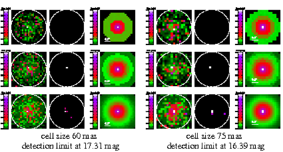
Figure 1: Monte Carlo simulations for two different camera setups that resemble the K’-band for NACO (right) and SINFONI (left) at the VLT. Upper panel: Snapshot of the simulation for the 0.11 KLF slope, power-law index $\Gamma=0.3$ and 24.67 Ks-magnitude cutoff Left: All stars visible. Middle: Only the detectable blend stars visible. Right: Average of all the 10⁴ simulation snapshots for the same setup. Middle & Lower panel: Same as top but for the 0.18 and 0.25 KLF slopes, respectively.

The simulations of the faint S-star cluster population was done by making use of the extrapolated KLF and star counts that go to K-magnitudes fainter than 18 (with a cutoff at 25). Sabha et al. (2012) distributed the stars in a $23\times 23$ grid corresponding to 529 cells with dimensions of $0.06^{\prime\prime}\times 0.06^{\prime\prime}$. The cell size corresponds to about one angular resolution element in K-band. So the simulations covers the inner $1.38^{\prime\prime}\times 1.38^{\prime\prime}$ projected region surrounding Sgr A*. Sabha et al. (2012) match the radial number density counts to the observed power-law index of $\Gamma=0.30\pm 0.05$ from Schödel et al. (2007). Their algorithm then fills each cell with its specified number of stars by choosing them randomly from a pool of stars created from the extrapolated KLF. Then the fluxes of the stars in each individual cell are added up and compared to the flux of the faintest star detected in that region until now. The simulations were carried out $10^{4}$ times in order to get reliable statistical estimates for the brightnesses in each resolution cell. Some of the results are depicted in Figure 1. The corresponding tables are given in Sabha et al. (2012) for the 0.06 arcsec cell size and here in Tabs. 1 and 2 for the 0.075 cell size. Sabha et al. (2012) find that especially towards the center - i.e. towards the position of SgrA* - this phenomenon occurs for a quarter to three quarters of cases simulated. This finding is consistent with the observations (Witzel et al. 2012, Dodds-Eden et al. 2011) that find offsets to the flux density towards SgrA* that are likely due to a time variable stellar contribution. Using the observed KLF and number density slopes the total number of stars in the simulated S-star cluster is consistent with the number of main sequence stars assumed in simulations by Freitag et al. (2006).

With these simulations Sabha et al. (2012) could show that the formation of blend stars has to be considered. These will contaminate the appearance of the S-star cluster at flux levels close to the confusion limit. This is especially important at positions close to Sgr A* where the number density counts peak. The authors also point out that due to the sky-projected velocity dispersion of the stars within the S-star cluster of about 600 km/s, these blend stars will last for about 3-4 years before the apparent line of sight clustering dissolves and the blend star fades away. So it requires proper motion measurements over a time significantly longer than 3 years to decide if an object is in fact a blend star or a single object for which reliable orbital parameters can be derived. Spectroscopy may be difficult since the objects are faint. Sabha et al. (2012) find that close to the center the probability of finding blend stars at any time is about 30%-50%. At the central position this effect may also give the illusion of high proper motions.

The phenomenon of blend stars clearly demonstrate that higher angular resolution, astrometric accuracy and point source sensitivity is required in order to further analyze the properties of the S-star cluster. In return these investigations also greatly improve 1) the derivation of the amount and the compactness of the central mass, 2) the determination of relativistic effects in the vicinity of Sagittarius A*, and 3) the determination of the abundance of e.g. massive stellar black holes in the central S-star cluster.

$\bullet$ Finding stars fainter than those that are known in order to probe the gravitational potential requires an angular resolution (at high sensitivity) beyond that achievable with current 8-10m telescopes. This will be possible with the interferometers LINC-NIRVANA and GRAVITY in the NIR or with METIS at the E-ELT in the MIR.

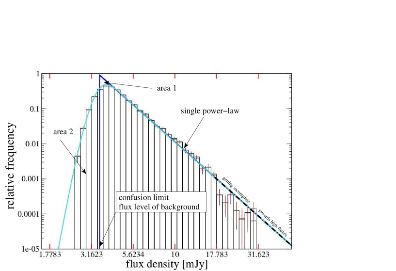
Figure 2: Here we show the best piecewise-constant probability density model for the flux densities of Sgr A* as presented by Witzel et al. (2012). The red error bars represent the uncertainty of the bin height for the total amount of 10 639 data points. In some cases there is a second bin height visible. Those and the black error bars belong to the average histograms of 1000 datasets with a total of 6774 data points, generated by randomly removing points from the full dataset. The dash-dotted blue line shows the extrapolation of the best power-law fit. The cyan line shows the power-law convolved with a Gaussian of a flux density distribution of 0.32 mJy width (see Witzel et al. 2012). The two areas labeled in the figure are equal in the corresponding non-logarithmic plot.

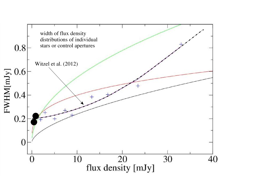
Figure 3: The measurement error as a function of flux density as presented by Witzel et al. (2012). The blue line is a quadratic fit to the measured flux distributions of the calibration stars used to calibrate SgrA* flux densities as presented by Witzel et al. (2012). The red line represents the power-law dependency given by Do et al. (2009). The green line and the black line show the dependency found by Dodds-Eden et al. (2011) for their aperture photometry and their PSF-fitting approach, respectively. The two black filled circles represent the measured widths of the flux density distributions at star-free control positions as described by Witzel et al. (2012).

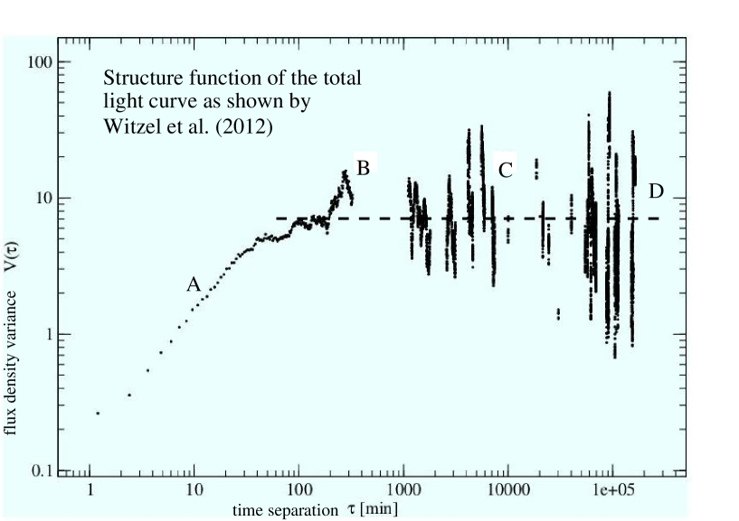
Figure 4: The structure function of the observed total light curve presented by Witzel et al. (2012). The time binning is 1.2 minutes. The flat region at large time separations has been indicated by a dashed line. Specific regions have been labeled: A: around 20 minutes - domain were significant deviations from a straight line occurs; B: around 1000 minute - day/night gap; C: around 10⁴ minutes - time difference between observing runs within a year; D: around few times 10⁵ minutes - difference between summer/winter runs.

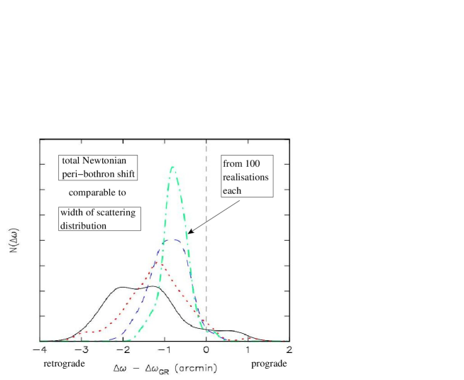
Figure 5: Histograms of the predicted change in S2’s argument of peri-bothron, $\omega$, over the course one orbital period (about 16 yr). The shift due to relativity, ($\Delta\omega$)_GR$\sim$11’, has been subtracted from the total; what remains is due to Newtonian perturbations from the field stars. Regions of residual prograde and retrograde shift are indicated. Each histogram was constructed from integrations of 100 random realizations of the same initial model, with field-star mass $m$ = 10  M_⊙ , and four different values of the total number: $N$ = 200 (solid/black); $N$ = 100 (dotted/red); $N$ = 50 (dashed/blue); and $N$ = 25 (dot-dashed/green). The average value of the peri-bothron shift increases with increasing $Nm$. As discussed by Sabha et al. (2012) there is a separate contribution that scales approximately as $\sim$1/$\sqrt{(}N)$ and that results in a variance about the mean value.

2.2 Orbital elements of high velocity stars

As laid out by Sabha et al. (2012), for faint stars close to the confusion limit the determination of their position will be affected by the presence of background stars with time variable clustering. The actual uncertainty in projected position, $\sigma_{\mathrm{position}}^{2}$, will be affected by several effects. Sabha et al. (2012) introduce $\sigma_{\mathrm{apparent}}^{2}$ as the apparent positional variation due to the photo-center variations of the star while it is moving across the projected distribution of fore- and background sources. In addition to this there may an effect due to stellar scattering resulting in a variation of positions described by $\sigma_{\mathrm{scattering}}^{2}$. This may also contain a significant positional displacement due to the fact that the stellar part of the gravitational potential may vary as a function of time due to the grainyness in the distribution of particularly the more massive stars. Finally, there is of course a systematic uncertainty $\sigma_{\mathrm{systematic}}^{2}$ that stems from establishing and applying an astrometric reference frame. Sabha et al. (2012) show how the different contributions can be derived or estimated such that information on $\sigma_{\mathrm{scattering}}^{2}$ can be obtained. In addition of making use of data obtained from 8-10m telescopes, one can alternatively make use of near-infrared interferometry with long baselines and measure $\sigma_{\mathrm{scattering}}^{2}$ directly.

Hence, measuring the time dependent position of S2 interferometrically with respect to brighter reference stars in the field, may allow us to observe either single scattering events or derivations from an elliptical orbit due to a varying underlying stellar fraction of the gravitational potential. Sabha et al. (2012) point out that if scattering events contribute significantly to the uncertainties in the determination of the orbits, we will require a larger number of stars to derive the physical properties of the medium through which the stars are moving. Averaging the results of $N$ stars that will then essentially sample the shape of the distributions shown in Figure 5 may therefore result in a $N^{-1/2}$ improvement in the determination of the extended mass. At the same time one will obtain information on the composition of the stellar environment the stars are moving through.

$\bullet$ Higher angular resolution observations as they will be possible with LINC-NIRVANA, GRAVITY in the NIR or METIS in the MIR will help to overcome some of the confusion due to photo-center shifts caused by fore- and background stars. Precise measurements of stellar trajectories are needed to distinguish between relativistic/Newtonian effects and effects due to resonant relaxation, i.e. stellar scattering or a variation of the stellar mass enclosed in the stellar orbits.

2.3 Faint states of Sagittarius A*

Witzel et al. (2012) collected all Ks-band observations that had been carried out with the VLT until 2011. The authors constructed a double logarithmic histogram in which a given flux density value is plotted against its relative frequency. The resulting flux density histogram is peaked and can be represented by a single power-law towards higher flux densities (Figure 2). Witzel et al. (2012) conclude that it is not possible to verify the evidence of an intrinsic turnover that would indicate the peaked shape of a log-normal distribution given the knowledge about the true error distribution in the determination of flux densities at the location of Sgr A* (see Figure 3). Therefore, having no evidence for a log-normal distribution for dim flux density states, the necessity of a break in the distribution to account for the highest flux densities vanishes. This is true even if one accepts the data selection by Dodds-Eden et al. (2011) and ignores the fact that basically all flux density values higher than 17 mJy are only due to a single bright event. Instead of a two state description of the flux density statistics of SgrA* Witzel et al. (2012) prefer a simple power law with a slope of $\alpha$ = 4.2$\pm$0.1 and an intrinsic x-axis offset of 3.57$\pm$0.1 mJy. The instrumental effects on the photometry lead to a detection limit - and since flux density is a positive quantity, this intrinsic power-law of SgrA* may break naturally very close to 0 mJy. Hence, a single power-law distribution describes the observable intrinsic flux densities well. This assumption is simpler and clearly needs less parameters than the broken distribution proposed by Dodds-Eden et al. (2011). It can not be excluded that the intrinsic flux distribution of SgrA* shows some structure at flux densities below the detection limit, i.e. between 0 mJy and 3.57 mJy. It may as well follow a log-normal distribution at very low flux densities. However, the log-normal distribution used in the model of Dodds-Eden et al. (2011) and a supportive evidence for a break in the observed flux density distribution can be ruled out by the improved investigation of Witzel et a. (2012).

$\bullet$ In oder to study the faintest flux density variations of SgrA* in the near-infrared it is required to overcome the confusion from fore- and background stars by increasing the angular resolution. This will be provided both by LINC-NIRVANA and GRAVITY. LINC-NIRVANA has the advantage of being an imaging interferometer allowing for prompt calibration and extraction of flux densities from images. A disadvantage is the beam-shape allowing for high angular resolution (for the Galactic Center from Arizona) in east-west direction, only. For GRAVITY, flux density variations at high time resolution needs to be extracted from the visibilies directly or from imaging/modeling with variable uv-plane coverage. In the MIR domain the high point source sensitivity of METIS at the E-ELT will allow to study faint flux density variations against the stellar and thermal confusion background.

2.4 High frequency quasi-periodicities

In Figure 4 we show the structure function of the entire light curve as investigated by Witzel et al. (2012). Following the typical shape of a structure function there is a transition from a high frequency white noise regime via a straight line passing a turnover at a characteristic time scale to a flat regime. We note that the first significant deviation from that straight line occures at a time scale of around 20 minutes. This is the same time scale that has previousely been pointed out as the time scale on which quasi periodic variations have been reported to happen on some occasions. While any firm statement on that time scale based on the structure function is hampered due to possible confusion from the window function, this time scale is supported by statistics and individual modeling of polarized flares, i.e. strong flux density excursions (Eckart et al. 2006, Meyer et al. 2006a,b, 2007; Zamaninasab et al. 2008, 2010, 2011).

$\bullet$ For ground based light curves confusion from the time windowing function cannot be overcome, unless very long continous light curves from the southern hemisphere at locations where SgrA* is circumpolar can be obtained. Alternatively flare statistics and modeling of individual flares in polarized light have to be employed to further investigate the signatures of relativistically orbiting matter close to the central black hole (within or close to the mid-plane seen in GRMHD simulations). Photo-center shifts as they will be measurable with GRAVITY as well as sub-mm VLBI observations will be useful to investigate the physics associated with the variability on short time scales.

2.5 Radio variability of Sagittarius A*

The accretion flow onto SgrA* is often modeled as a relativistic magneto hydrodynamic flow (GRMHD) with a central mid-plane close to SgrA* where the densities and magnetic field strengths are likely to be highest (Moscibrodzka et al. 2009, 2011, Dexter et al. 2010, 2012). These models assume that the emission arises in a luminous flow region with an outer radius of about 200$\mu$as, whereas the mid-plane covers the central few 10$\mu$as (i.e. a few Schwarzschild radii). The image of this structure is severely scatter broadened at radio wavelengths longward of 3 mm. Radio variability may and will occure from individual regions (individual source components) all over the extended accretion flow. At mm- and sub-mm-wavelengths this variability will provide a significant confusion background against which the central accretion phenomena close or within the mid-plane has to be detected. Characteristic frequency behaviours like adiabatic expansion of source components can be clearly distinguished from that confusion by following them over a frequency range that is beyond the bandwidth of individual receiving channels. A detailed discussion of this problem is given in Eckart et al. (2012).

$\bullet$ Sub-mm observations over the largest possible frequency range (as they are possible with ALMA) will help to distinguish mid-plane intrinsic variability phenomena from the confusion originating within the more extended accretion flow

2.6 X-ray variability of Sagittarius A*

In the X-ray domain it is difficult to study weak flux density variations. For faint states the flux density is dominated by the thermal Bremsstrahlung component with an angular diameter of about one arcsecond (Baganoff et al. 2001, 2003). Studying fainter flux density levels will allow an improved investigation of the detailed correlation between the NIR and X-ray light curves.

$\bullet$ Future missions with sub-arcsecond angular resolution and high sensitivity in the X-ray domain will allow to distinguish low flux density variations of SgrA* against confusion from the extended thermal Bremsstrahlung background component.

3 IMPLICATIONS FOR INSTRUMENTATION

The described confusion effects clearly demonstrate the necessity of higher angular resolution and point source sensitivity for future investigations of the S-star cluster and the derivation of the amount and the compactness of the central mass as well as the determination of relativistic effects in the vicinity of Sgr A*. In the NIR/MIR domain these implications are clearly met by the upcomming systems GRAVITY at the VLTI, LINC-NIRVANA at the LBT and METIS at the E-ELT.