Time-Correlated Structure in Spin Fluctuations in Pulsars

Abstract

We study statistical properties of stochastic variations in pulse arrival times, timing noise, in radio pulsars using a new analysis method applied in the time domain. The method proceeds in two steps. First, we subtract low-frequency wander using a high-pass filter. Second, we calculate the discrete correlation function of the filtered data. As a complementary method for measuring correlations, we introduce a statistic that measures the dispersion of the data with respect to the data translated in time. The analysis methods presented here are robust and of general usefulness for studying arrival time variations over timescales approaching the average sampling interval. We apply these methods to timing data for 32 pulsars. In two radio pulsars, PSRs B1133+16 and B1933+16, we find that fluctuations in arrival times are correlated over timescales of $10-20$ d with the distinct signature of a relaxation process. Though this relaxation response could be magnetospheric in origin, we argue that damping between the neutron star crust and interior liquid is a more likely explanation. Under this interpretation, our results provide the first evidence independent from pulsar spin glitches of differential rotation in neutron stars. PSR B0950+08, shows evidence for quasi-periodic oscillations that could be related to mode switching.

1 Introduction

Radio pulsars are superb clocks. The regularity of the arrival times of the pulsed emission, upon barycentering, subtraction of proper motion, and gradual spin down, rivals atomic clocks in stability. Perhaps even more interesting are the imperfections of pulsars as clocks; variation in pulse arrival times, timing noise, is present at some level in all pulsars, and has remained unexplained since the discovery of pulsars in 1967. Timing noise is a very complex process, and there appear to be many contributing factors; Hobbs et al. (2010) and Cordes & Downs (1985) have shown that the complexity of timing noise cannot be explained by high frequency random walks in the pulsar spin parameters (see, for example, Boynton et al. 1972; Cordes 1980). Possible contributors to timing noise include variable coupling between the crust and the liquid interior (Alpar et al., 1986; Jones, 1990), stochastic adjustments to the star’s figure (Cordes, 1993), variations in the external electromagnetic spin-down torque on the star (Cheng, 1987a, b; Urama et al., 2006; Lyne et al., 2010), and time variability of the interstellar medium between the pulsar and Earth (Liu et al., 2011).

A neutron star is a dynamic system consisting of a rigid crust, a liquid interior, and an active magnetosphere. Variations in the spin rate of the crust are the result of driving torques on the crust, filtered by the response of the system to those torques. Generally in noisy systems it is possible to determine properties of the response function without knowledge of the forcing function. For example, thermal fluctuations of the current in a circuit containing a resistor of resistance $R$ in series with a capacitor of capacitance $C$ can be used to measure the circuit’s intrinsic decay time $RC$, independent of the processes that drive the current fluctuations. In this paper we develop techniques with which to measure properties of the response function of the neutron star system.

Using timing noise to probe the neutron star system is an old idea. For a neutron star with a damped rotational mode associated with, for example, friction between the crust and a portion of the liquid interior, stochastic perturbations from rotational equilibrium by the noise process would never relax completely. In this case, decoupling by fluctuations at frequencies higher than the damping frequency $\tau_{d}^{-1}$ would increase the spectral power for all frequencies above $\tau_{d}^{-1}$ by a magnitude determined by the ratio of the moments of inertia of the crust and the liquid to which it is imperfectly coupled (Lamb et al., 1978). Past studies of timing noise power spectra have not revealed structure beyond the power-law that is the hallmark of a noisy process, that is, no deviations from rigid-body rotation have yet been detected (Boynton & Deeter, 1979; Boynton, 1981; Boynton et al., 1984). The only evidence to date that neutron stars do not rotate rigidly comes from a very different phenomenon than timing noise: the glitches, sudden increases in spin rate (see, for example, Lyne et al. 2000), whose occurrence and subsequent recovery have been attributed to variable coupling between the crust and the liquid interior (see, e.g., Alpar et al. 1984; Link et al. 1993; Pizzochero 2011). Why neutron stars have not shown signatures of deviations from rigid-body rotation in their noise spectra has been an important open question in neutron star physics for over three decades.

Since the early work on timing noise, the quantity and quality of data have increased. In the largest and most comprehensive study of timing noise to date, Hobbs et al. (2010) presented timing residuals of 366 pulsars over nearly 40 years, some with nearly daily monitoring, mainly by the Lovell Telescope at Jodrell Bank. Here we revisit the issue of using timing noise to identify properties of neutron star response with these high-resolution data using methods applied in the time domain to 32 radio pulsars. In two radio pulsars, PSRs B1133+16 and B1933+16, we find that fluctuations in arrival times are correlated over timescales of $10-20$ d with the distinct signature of a relaxation process. Though the relaxation response could be magnetospheric in origin, we argue that damping between the neutron star crust and interior liquid is a more likely explanation. Under this interpretation, our results provide the first evidence independent from pulsar spin glitches of differential rotation in neutron stars.

While this paper focuses on identification of signatures of the underlying physical processes responsible for pulsar timing fluctuations, the mathematical characterization of timing noise also plays a crucial role in efforts to detect gravitational waves in pulsar timing arrays such as the North American Nanohertz Observatory for Gravitational Waves NANOGrav (http://www.nanograv.org), the Parkes Pulsar Timing Array PPTA ( http://www.atnf.csiro.au/research/pulsar/ppta/), and the European Pulsar Timing Array EPTA ( http://www.epta.eu.org). In particular, if the underlying power spectrum of timing noise is known, the signal-to-noise ratio for the gravitational wave background could be substantially improved (van Haasteren et al., 2009).

In §2 we describe the data that we analyzed. In §3 we describe our analysis methods. In §4 we present results of the analysis for five radio pulsars. In §5 we discuss our results. The details of the analysis methods, examples of applications to simulated data sets, and tests of robustness are presented in the Appendix.

2 Data

The Green Bank data were collected using a 25-m radio telescope at the National Radio Astronomy Observatory, Green Bank, West Virginia. This telescope monitored the pulsars on a near daily basis from 1989 through 1999. Observations followed a fixed daily schedule (adjusted a few times over the course of the program). Integration time depended on source strength, but was typically of order 40 minutes, and was divided into several subintegrations. For each of two linear polarizations, a filter bank produced total-power values for each of sixteen 1-MHz spectral channels across a band centered at 610 MHz. (The channels were not completely contiguous due to radio frequency interference considerations.). The two polarizations were balanced (using measured system noise), summed, and folded modulo the pulse period using the Princeton Mark 3 data acquisition system (Stinebring et al., 1992). This procedure produced a single pulse profile for each spectral channel in each subintegration. Off-line, the folded data profiles were cross-correlated with a high precision standard template to produce pulse times of arrival (TOAs). The TOAs from all channels and all subintegrations of any given pulsar on any given day were averaged to produce a single effective daily TOA, which was used for the present analysis. These TOAs were then analyzed with the tempo2 software package (Hobbs et al., 2006) to obtain the timing residuals, using the JPL DE405 ephemeris. In each case, fits were made for position, proper motion, rotational frequency, and rotational frequency derivative.

The Jodrell Bank data were collected using the 13-m Lovell Radio Telescope with nearly daily observations from 1991 to 2008. Observations were made at 610 MHz, with a 4 MHz bandwith. 30-60 minutes of observations were made for each pulsar, depending on the flux density of each object, and then divided into 1-3 minute subintegrations. The subintegrations were averaged to produce a single profile, which was convolved in the time domain with the corresponding pulse template to produce TOAs (Hobbs et al., 2004). These TOAs were then analyzed with the tempo2 software package (Hobbs et al., 2006) to obtain the timing residuals, using the JPL DE200 ephemeris.

3 Analysis Methods

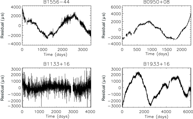
Timing noise appears as stochastic wander of the pulse arrival time, with respect to a deterministic spin-down model, over all timescales; examples are shown in Fig. 1. In most cases, the dominant effect is that of low-frequency variation over years. To study possible correlations over much shorter timescales, we work in the time domain and first subtract the slow wander of the timing residuals through application of a high-pass filter. We then perform two types of correlation analyses on these filtered (that is, “whitened”) data.

3.1 High-Pass Filtering

Figure 1: Timing residuals in microseconds for four pulsars, showing typical long-period wander. The data are from the Jodrell Bank and Green Bank data archives (see Table 1). The residuals were obtained using the tempo2 software package (Hobbs et al. 2006).

We divide the time series into contiguous non-overlapping intervals of width $W$ and calculate the average value of the residuals in each interval. Using unweighted least-squares fitting, we fit the average values with a cubic spline, and subtract the spline from the original time series to obtain the whitened residuals. More details and examples of this filtering method are given in the Appendix. For most data sets, a broad range in choices of the filter width $W$ effectively removes long-period wander without introducing spurious correlations.

3.2 Discrete Correlation Function

The data we analyze are unevenly sampled, and often contain large gaps. It is desirable to measure autocorrelations without having to bin the data, which would restrict our analysis to a timescale no shorter than the longest gap in the data and would entail a severe loss in time resolution. Unevenly-sampled data is readily handled with the discrete correlation function ${\rm DCF}(\tau)$ (Edelson & Krolik, 1988), which we calculate as follows. For a set of arrival time residuals $\delta t_{i}$ measured at times $t_{i}$, we construct the matrix

$${\rm DCF}_{ij}=\frac{(\delta t_{i}-\overline{\delta t})(\delta t_{j}-\overline{\delta t})}{\sigma^{2}},$$ (1)

where $\overline{\delta t}$ is the mean of the data set and $\sigma$ is its standard deviation (the choice of normalization is arbitrary). This matrix is calculated for all possible pairs $(\delta t_{i},\delta t_{j})$, each of which is associated with the time difference $\Delta t_{ij}\equiv t_{j}-t_{i}$ between the $i$-th and $j$-th measurements. (Here and in the following, $\delta t$ will denote residuals, and $\Delta t$ will denote differences in measurement times). Suppose that there are $M$ pairs that satisfy the condition

$$\tau-\Delta\tau/2\leq\Delta t_{ij}<\tau+\Delta\tau/2,$$ (2)

where $\Delta\tau$ is the width of the sampling window. The discrete correlation function is the time average of eq. (1) for the pairs that satisfy eq. (2), that is,

$${\rm DCF}(\tau)=\frac{1}{M}\sum{\rm DCF}_{ij}.$$ (3)

Points that do not fall in the sampling window do not contribute to ${\rm DCF}(\tau)$. The window size is chosen to maximize resolution without loss of statistical significance; in practice, $\Delta\tau$ can be taken to be almost as small as the average sampling time. This procedure uses every data point, without any significant penalty in resolution due to occasional large gaps in the data. The values of $\tau$ that are used are binned in units of $\Delta\tau$. The standard uncertainty in the ${\rm DCF}(\tau)$ is (Edelson & Krolik, 1988)

$$\sigma_{\rm DCF}(\tau)=\frac{1}{M-1}\left\{\sum\left[{\rm DCF}_{ij}-{\rm DCF}(\tau)\right]^{2}\right\}^{1/2}.$$ (4)

3.2.1 Lagged Dispersion

As another statistic with which to measure correlations, we introduce the lagged distribution function, $\rm{LDF}\{\delta t,\tau\}$, the distribution of fluctuation differences separated in time by a lag $\tau$. Correlations in the data can be studied with the lagged dispersion ${\rm LD}(\tau)$, which we define as the dispersion of the lagged distribution function. The LD has the following properties for a data set that is correlated over a timescale $\tau_{c}$ (and without a resonance). Because the time series will resemble itself to some extent upon time translation by times $\tau<\tau_{c}$, the $\rm{LDF}\{\delta t,\tau\}$ will be relatively narrow, and hence $LD(\tau)$ will be relatively small. For $\tau>\tau_{c}$, the dispersion is larger because the data around time $t+\tau$ are uncorrelated with the data around time $t$; in this case $\rm{LDF}\{\delta t,\tau\}$ is broader than at low lag, and ${\rm LD}(\tau)$ asymptotes to some maximum value as $\tau$ is increased. If the data series is simply noise, there will be no statistically-significant variations in ${\rm LD}(\tau)$ with $\tau$, since the data contain no timescale. A general increase of ${\rm LD}(\tau)$ up to a lag $\tau\simeq\tau_{c}$ indicates that the series is correlated over a timescale $\sim\tau_{c}$. Oscillations in the data appear also as oscillations in the LD.

To handle uneven sampling, we construct ${\rm LD}(\tau)$ in a similar way as the $DCF(\tau)$:

$${\rm LD}(\tau)\equiv\frac{1}{M-1}\sum(\delta t_{ij}-\overline{\delta t})^{2},$$ (5)

where $\delta t_{ij}\equiv\delta t_{i}-\delta t_{j}$. As before, the product is over the set of $M$ elements that satisfies eq. (2), in which each element of the set is associated with the lag value $\tau$. The mean $\overline{\delta t}$ in eq. (5) is defined as

$$\overline{\delta t}\equiv\frac{1}{M}\sum\delta t_{ij}.$$ (6)

The LD is mathematically similar to the structure function used in studies of the turbulent interstellar plasma (e.g., Rickett 1990; You et al. 2007).

The standard uncertainty in ${\rm LD}(\tau)$ is

$$\sigma_{\rm LD}(\tau)=\frac{1}{M-1}\left[\sum(\delta t_{ij}-\overline{\delta t})^{2}-\rm LD(\tau)\right]^{1/2}.$$ (7)

In the Appendix, we illustrate the usefulness of the DCF and the LD, in combination with high-pass filtering, to identify short-timescale correlations that are not readily identified with Fourier techniques. We find that high-pass filtering of the time series followed by calculation of the DCF or LD is a robust method for identifying an intrinsic relaxation timescale $\tau_{c}$, provided the following conditions are satisfied:

$$\Delta t_{\rm samp}<\tau_{c}<\tau_{\rm wander},$$ (8)

where $\Delta t_{\rm samp}$ is the mean sampling interval and $\tau_{\rm wander}$ is the shortest timescale of the wander. If the first inequality is not satisfied, then the time resolution of the data is not sufficient to resolve the correlation timescale. If the second condition is not met, then the correlation cannot be disentangled from the wander. In practice, we must also require

$$\tau_{\rm corr}<W<\tau_{\rm wander},$$ (9)

to ensure that the filter removes the wander but not the correlation. In the extreme case of $W\sim\tau_{\rm samp}$, the filtering method introduces spurious anti-correlations, indicating that the choice of $W$ is too small.

4 Correlation Analyses

Name	Observatory	Period (s)	$\tau_{\rm age}$ (Myr)	Data Span (d)	No. of Observations
$B0136+57$	GB	0.27	0.4	3558	2685
$B0329+54$	JB	0.72	5	4313	3884
$B0355+54$	JB	0.16	0.6	3376	855
$B0525+21$	GB	3.75	1	3387	1346
$B0628-28$	GB	1.24	3	3177	1593
$B0736-40$	GB	0.37	4	2312	1056
$B0740-28$	JB	0.17	0.2	1820	1631
$B0818-13$	GB	1.24	9	3402	1680
$B0823+26$	GB	0.53	5	2113	1025
$B0835-41$	GB	0.75	3	3561	1948
$B0950+08$	GB	0.25	20	2312	1223
$B1133+16$	JB	1.19	5	4043	3956
$B1237+25$	GB	1.38	20	2267	923
$B1508+55$	GB	0.74	2	3561	1923
$B1556-44$	GB	0.26	4	3405	2498
$B1641-45$	GB	0.46	0.4	3556	2071
$B1642-03$	JB	0.39	3	6248	5555
$B1749-28$	GB	0.56	1	3554	2205
$B1818-04$	GB	0.60	2	3558	1877
$B1822-09$	GB	0.77	0.2	1091	476
$B1831-03$	GB	0.69	0.3	3396	1711
$B1859+03$	GB	0.66	1	3176	1762
$B1911-04$	GB	0.83	3	2310	1224
$B1919+21$	GB	1.34	20	3548	2567
$B1929+10$	JB	0.23	3	4267	3800
$B1933+16$	JB	0.36	0.9	6249	5377
$B1946+35$	GB	0.72	2	2171	1163
$B2016+28$	GB	0.56	60	1885	951
$B2020+28$	GB	0.34	3	1953	1238
$B2045-16$	GB	1.96	3	1705	699
$B2111+46$	GB	1.02	20	3544	1986
$B2217+47$	GB	0.54	3	3556	1971

Table 1: The pulsars to which we have applied the analysis techniques of this paper. JB - Jodrell Bank timing data, from the 13m dish with an observing frequency of 610 MHz, with a 4 MHz bandwidth, using 30-60 min observing sessions. GB - Green Bank timing data, from telescope 85-3 (25m diameter), with an observing frequency of 610 MHz and 16 MHz bandwith, with typical observation sessions of $\sim$ 40 min. The pulsar parameters given are from ATNF Pulsar Catalog (http://www.atnf.csiro.au/people/pulsar/psrcat/).

We have applied the methods of §3 to the 32 radio pulsars of Table 1. We apply a high-pass filter to the residuals, and then calculate the ${\rm DCF}$ and the ${\rm LD}$. In most cases, we see no statistically significant correlations after the data are whitened. Here we present results for PSRs B1133+16, B1933+16, B0525+21, B1556-44, B0950+08, as particularly interesting examples that show correlated structure in their time series.

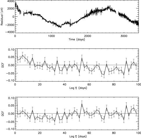
PSRs B1133+16 and B1933+16. These two pulsars have been monitored almost daily with the 12.8 m telescope at Jodrell Bank, usually at 610 MHz. Timing residuals for PSR B1133+16 over about 4000 days, and PSR B1933+16 over about 6000 days, are shown in Fig. 2. We begin with these pulsars because they show particularly interesting correlations in their times series.

Figure 2: Timing fluctuations in PSR B1133+16, in microseconds. Second panel - timing fluctuations after subtraction of the long-term wander evident in the top panel, using a filter width $W=400$ days. The uncertainties are comparable in magnitude to the fluctuations, and are not shown for clarity. The gaps in the data sets are on account of equipment upgrades; our analysis techniques enable us to use data on both sides of the gaps. Third panel - DCF of the whitened residuals. Fourth panel - LD of the whitened residuals. Bottom panel - power spectrum of the 1700 day span of unwhitened residuals (see text).

Figure 3: Same as Fig. 2, for PSR B1933+16. The filter width is $W=120$ d, for which the correlations over timescales of $\sim 20$ d are most clearly seen. The power spectrum in the bottom panel is for the 1400 day span of unwhitened residuals (see text).

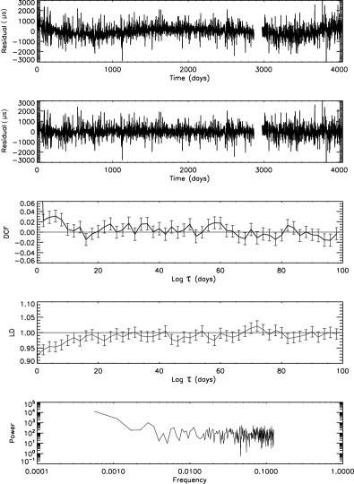
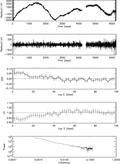
In Figs. 2 and 3 (3rd panel) we show the DCFs for B1133+16 and B1933+16, after whitening with filter widths $W$ of 400 d and 120 d, respectively. Uncertainties were obtained from eq. (4). (All uncertainties in this paper are 1-$\sigma$). The DCF for B1133+16 shows highly significant, non-periodic correlations over a timescale $\tau_{c}\sim 10$ d, with the distinct structure of a relaxation process (see Appendix). B1933+16 shows similar correlations, over a timescale $\tau_{c}\sim 20$ d. From the calculated uncertainties, shown in the figures, the confidence level of the detected correlations is high. We estimate the correlation significance to be

$$S=\prod_{i}\frac{{\rm DCF}(\tau_{i})}{\sigma(\tau_{i})},$$ (10)

where the product is over all values of $\tau_{i}<\tau_{c}$, the inferred correlation timescale. The quantity $S$ should give an approximate measure of the significance of the result in units of the (typical) statistical uncertainty of each data point. For B1133+16, the correlation over $\tau_{c}=10$ is seen over the first four bins of width $\Delta\tau=2$ d, giving $S=24.5$. For B1933+16, the correlation over $\tau_{c}=20$ is seen over the first nines bins of width $\Delta\tau=2$ d, giving $S=31.2$. These values of $S$ indicate very high statistical significance. As a check, we obtain a lower limit on the significance with a bootstrapping method. We create an ensemble of data sets in which the time-ordering of the whitened residuals is randomly shuffled. The DCF is calculated for the shuffled data, with $\Delta=2\tau$ d for both pulsars. We calculate the significance $S_{\rm shuffled}$ for $0\leq\tau\leq\tau_{c}$ (the first four bins for PSR B1133+16, and the first nine bins for PSR B1933+16). We then ask: what fraction of shuffled sets give $S_{\rm shuffled}>S$? Under the null hypothesis of uncorrelated data, $S_{\rm shuffled}$ is comparable to $S$, since $S$ represents one particular realization. In $10^{4}$ shufflings for each data set, the null result was never realized. We therefore estimate the statistical significance of the detected correlations to exceed $1-10^{-4}$, consistent with the values of $S$ obtained above. This estimation method has the advantage that nothing is assumed about the underlying statistics of the data, rather, the data themselves are used to evaluate the likelihood of the null hypothesis.

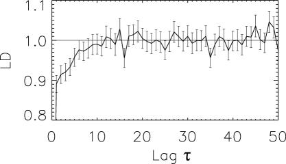
In Figs. 2 and 3, we show ${\rm LD}(\tau)$ for PSRs B1133+16 and B1933+16. The value of LD for uncorrelated data is calculated by averaging many shufflings of the data; this value is used to normalize ${\rm LD}(\tau)$ shown in the figures (see Appendix A3). For B1133+16, we find that ${\rm LD}(\tau)$ is significantly lower than what we expect from the null hypothesis out to $\tau\simeq 10$ d, in support of the DCF result. B1933+16 is very similar, but indicates a relaxation timescale $\tau_{c}\simeq 30$ d, consistent with the DCF.

The power spectra of the unwhitened data do not show the correlations that our time-domain analysis has revealed. Gaps in observations of 4-5 days are frequent for B1133+16, and several gaps of 8-16 days are present. To obtain a power spectrum without interpolating data, we have chosen a span of data approximately 1700 days in length, with gaps no longer than four days. The power spectrum of the timing residuals are shown in Fig. 2 (bottom panel), using uniformly weighted bins of width four days. The spectrum is generally white, with some excess power at low frequencies. No high frequency features or spectral breaks are evident. For PSR B1933+16, we select a segment of data spanning 1400 days, also placed in bins of width four days, to calculate the power spectrum shown in Fig. 3 (bottom panel). The red spectrum corresponds to the low-frequency wander visible in the timing residuals (Fig. 3). The Fourier transform spreads the power over all frequencies, obscuring correlations that are more readily identified in the time domain.

The two complementary and independent statistics we have used here, ${\rm DCF}(\tau)$ and ${\rm LD}(\tau)$, measure different properties of the data. The DCF measures the extent to which the data set compares to itself upon translation in time, while the LD measures the extent to which the distribution of fluctuation differences widens as the data decorrelate for larger lags. These two different statistics give consistent results for PSRs B1133+16 and B1933+16. Several tests of the robustness of these results are given in the Appendix. In particular, the whitening process cannot introduce spurious correlations at timescales shorter than the window width. The filter width of $W=400$ d used for the analysis of PSR B1133+16 is a factor of $\sim 40$ larger than the derived correlation time. The filter width of $W=120$ d used for the analysis of PSR B1933+16 is a factor of $\sim 6$ larger than the correlation time.

Figure 4: Top panel - Timing residuals for PSR B0525+21, in microseconds. Middle panel - residuals after whitening with W=100 days. Bottom panel - The DCF of the whitened data, showing variability over $\sim 10$ d.

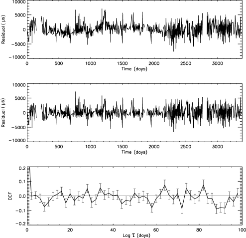
PSR B0525+21. Timing residuals are shown in Fig. 4 (top panel). The wander in the timing noise occurs over timescales $\gtrsim 300$ days. Upon whitening with a filter width $W=100$ days, the DCF (bottom panel) shows variability over timescales of $\sim 10$ d, but no evidence of relaxation. Relaxation response, if present, could be overwhelmed by the variability.

PSR B1556-44. Timing residuals are shown in Fig. 5 (top panel). DCFs for this pulsar are shown in Fig. 5 for $W=100$ (middle panel) and 50 days (bottom panel). For $W=100$ days, the DCF shows variability over $\sim 10$ d. With $W=50$ days, more wander is removed, but variability over timescales $\hbox{${{}_{\displaystyle>}\atop{}^{\displaystyle\sim}}$}10$ d is still evident (bottom panel). As for PSR B0525+21, any possible signature of relaxation response might be overwhelmed by the variability.

Figure 5: Top panel - Timing residuals for PSR B1556-44. Middle panel - The DCF after whitening with a filter width $W=100$ d. Variability over $\hbox{${{}_{\displaystyle>}\atop{}^{\displaystyle\sim}}$}10$ d is evident. Bottom panel - The DCF with $W=50$ days. More wander has been removed, but variability remains.

Figure 6: Top panel - Timing residuals for PSR B0950+08, in microseconds. Middle panel - The residuals after whitening with a filter width $W=100$ d. Bottom panel - The DCF of the whitened residuals, showing variability over timescales comparable to observed pulse mode changes (Shabanova & Shitov, 2004).

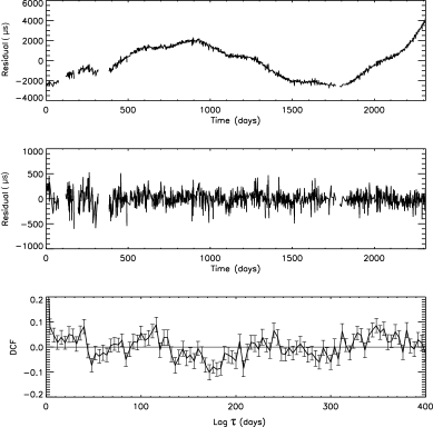
PSR B0950+08. Timing residuals are shown in Fig. 6. Upon whitening the data, the DCF of this pulsar shows both correlations and anti-correlations (Fig. 6, bottom panel), associated with quasi-periodic variability over a timescale of $\hbox{${{}_{\displaystyle<}\atop{}^{\displaystyle\sim}}$}100$ d. The pulse profile of PSR B0950+08 changes modes over timescales comparable to those identified in the DCF (Shabanova & Shitov, 2004); the variability in the DCF could be directly related to mode changing.

5 Discussion

We find strong evidence for correlation of timing residuals over timescales less than $\sim 10$ d in PSR B1133+16, and $\sim 20$ d in PSR B1933+16, indicative of relaxation response in the neutron star system of crust, core, and magnetosphere. While it is possible that the correlations are created by variable torques in the magnetosphere, we consider this possibility to be unlikely. The basic timescale in the magnetosphere is the light travel time across the light cylinder, which is comparable to the spin period. For the observed correlations to be magnetospheric in origin, the magnetosphere must have a relaxation time of weeks. Such a long relaxation time is difficult to explain on physical grounds. Lyne et al. (2010) have shown that many stars exhibit changes in spin-down rate in association with pulse-shape changes, clear evidence that the magnetosphere is dynamic, but these changes always occur much more quickly than $\sim 10$ d. PSR B1133+16 and PSR B1933+16 show no evidence for such modes changes, though PSR 1133+16 does show nulling. Mode changes would show both correlations and anti-correlations, unlike B1133+16 and B1933+16, which show only correlations.

The correlations cannot be due to time variability of the interstellar medium. The delay in the arrival time of a pulse of frequency $\nu_{\rm MHz}$ due to dispersion in the interstellar medium is (Lyne & Graham-Smith, 2005)

$$\Delta t_{ISM}=4.15\times 10^{6}\,\rm{MHz}^{2}\,\rm{pc}^{-1}{\rm cm}^{3}\,\rm{ms}\,\times\nu_{MHz}^{-2}\times DM,$$ (11)

where DM is the dispersion measure (cm^-3 pc). The dispersion measure is calculated during multi-wavelength observations for B1133+16 and B1933+16, and used to subtract the delay as part of the timing solution. The time derivative of the dispersion measure has been measured from long-term monitoring: $d(DM)/dt\sim 8\times 10^{-4}\rm{cm}^{-3}\,\rm{pc}\,\rm{yr}^{-1}$ for B1133+16, and $\sim 2.3\times 10^{-3}\,\rm{cm}^{-3}\,\rm{pc}\,\rm{yr}^{-1}$ for B1933+16 (Hobbs et al., 2004). This variability of the electron density produces small fluctuations in the arrival time delay, on the order of $10\,\rm{\mu}\rm{s}\,\rm{yr}^{-1}$. To estimate the maximum effect of variations of the interstellar medium, we superimposed a sine wave of amplitude 10 $\mu$s with period 10 d on our whitened data. No detectable signal is introduced into either the DCF or the LD.

An alternative explanation is that the correlations found for PSRs B1133+16 and B1933+16 are due to damping between the neutron star crust and interior liquid as the system is excited, presumably often, away from a state of rotational equilibrium that is never reached. In this picture, our results provide the first evidence independent from pulsar spin glitches of differential rotation in neutron stars. In support of this interpretation, we note that the measured correlation times are comparable to the post-glitch recovery timescales measured in many pulsars (e.g., Lyne et al. 2000).

The methods introduced here are also generally useful for identifying quasi-periodic processes that occur over timescales of days. PSR B0950+08 is a particularly clear example, showing alternating correlations and anti-correlations in the DCF. This star exhibits mode changes over a similar timescale (Shabanova & Shitov, 2004), and so the DCF appears to be showing magnetospheric effects. Though not as strong as PSR B0950+08, PSRs B0525+21 and B1556-44 also show evidence for variability.

For most of the pulsars in Table 1, we find no evidence of relaxation behavior. In order to resolve correlation timescales of $\sim 10$ d, nearly daily sampling is required. Most of the pulsars that we have analyzed do not have the high sampling rates of PSRs B1133+16 and B1933+16. These pulsars with lower sampling rates might have short-timescale correlations that are not detectable yet with the methods used here. For data which contain relaxation and periodicity over similar timescales, it is not possible to remove the wander without removing any non-periodic correlations that may exist.

The analysis methods applied are suitable for seeking time correlated structure in any noisy time series (see, e.g., Fukumura et al. 2010 for a recent application of autocorrelation methods to the analysis of astronomical data). For pulsar timing noise in particular, these techniques show promise for distinguishing effects that might be magnetospheric in origin, such as mode switching, from those effects that are directly related to rotational response of the stellar interior. Mode switching, for example, is now known to be related to sudden changes in magnetospheric torque in many pulsars (Lyne et al., 2010). This effect can be seen as quasi-periodic behavior of the DCF, as we have shown with PSR B0950+08. By contrast relaxation response, as seen in PSRs B1133+16 and B1933+16, is more naturally attributed to internal dynamical degrees of freedom. An in-depth study of relaxation response in the context of a physical model is in progress. The techniques developed in this paper may also be used to detect precession and oscillation modes in pulsar timing data.

Appendix A Examples and Tests

In this Appendix we describe the analysis techniques used in this paper in more detail and present many examples and tests of robustness. Synthetic data sets are generated to simulate the properties of real radio pulsar timing data. We also discuss a simple physical model for random spindown torques that captures the essential features of the detected correlations.

A.1 Whitening with a High-Pass Filter

Figure 7: Top panel - Simulated residuals (arbitrary units) consisting of 10 sine waves, an arbitrary 5th order polynomial, and Gaussian noise, and the corresponding ACF. Second panel - Whitened data with a filter width $W=300$. Third panel- Further whitening with filter width $W=150$. Bottom panel- Further whitening with filter width $W=75$.

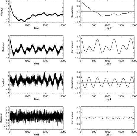
To illustrate the effects of the high-pass filter that we use, we construct simulated timing residuals $\delta t(t)$ consisting of periodic functions, quasi-periodic wander and gaussian noise,

$$\delta t(t)=\sum_{i}\left(\frac{A_{i}}{\omega_{i}}\sin(\omega_{i}t+\phi_{i})\right)+P(t)+N(t),$$ (12)

where $A_{i}$, $\omega_{i}$, and $\phi_{i}$ are the amplitude, frequency, and phase, respectively, $P(t)$ is an arbitrary polynomial function, and $N(t)$ is gaussian noise. $A_{i}$ and $\phi_{i}$ are randomly generated values. The sine waves are weighted by the frequency $\omega_{i}$ to produce a red power spectrum, similar to that of typical pulsar data. An example of a simulated time series is shown in Fig. 7 (top panel), using a sum of 10 sine waves. For this example, we choose frequencies $\omega_{i}=\omega_{1}/i$, where $i$ is an integer, and a weighting of $\omega_{i}^{-1}$. The maximum frequency is $\omega_{1}=0.32$ (period=19.6), and and the minimum frequency is $\omega_{10}=6.25\times 10^{-4}$ (period=$10^{4}$).

We now whiten the synthetic data as follows. We divide the time series into contiguous non-overlapping intervals of width $W$ and calculate the average value of the residuals in each interval. Using unweighted least-squares fitting, we fit the data in each interval with a cubic spline and subtract it from the original time series to obtain the whitened residuals. The effect of whitening for different values of the filter width $W$ can be seen by calculating the autocorrelation function of the whitened residuals. The autocorrelation function measures the similarity of a time series to itself upon translation in time by a given lag $\tau$,

$$ACF(\tau)=\sum_{t}\frac{(X_{t}-\mu)(X_{t+\tau}-\mu)}{\sigma^{2}},$$ (13)

where $X_{t}$ is the measured signal at time $t$, $\mu$ is the mean of $X_{t}$, and $\sigma$ is the square root of the variance of $X_{t}$. In this example, for $W=300$ the polynomial has been removed well, but significant periodicity remains in the time series (Fig. 7, 2nd panel). For $W=150$, some of the periodicity has been removed, but high frequency components are still apparent (Fig. 7, 3rd panel). Using a filtering parameter $W=75$ removes almost all of the wander in the time series, leaving a correlation function consistent with Gaussian noise (Fig. 7, 4th panel). Recall that the highest-frequency sine wave in the series has a period of 19.6, less than $W$, but the high-frequency components have been suppressed in proportion to the period.

Figure 8: Autocorrelation function of the simulated time series in Fig. 7 (top panel), after whitening with $W=20$, showing anti-correlation at low lag, the signature of overwhitening. The anti-correlation is strongest for lags $\sim W/2$.

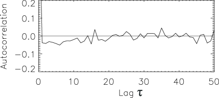
Anti-correlations arise if $W$ is too small, comparable to the sampling interval. In this case, the cubic spline begins to fit the noise, introducing spurious power at high frequencies. This results in a whitened time series which is anti-correlated for lags $\tau<W$ (Fig. 8), as fitting the noise produces residuals which are more likely to be of opposite sign. To see this, consider the limiting case in which each bin of width $W$ contains only two points. The average value of each bin is subtracted from the time series, resulting in data that are anti-correlated for a lag $\tau=1$. In general, the anti-correlation due to overwhitening is strongest for a lag $\tau\simeq W/2$. This distinct signature allows us to easily determine if the selected filter width $W$ is too small. As a general rule, we need to keep $W$ at least several times larger than the average sampling interval.

A.2 Comparison of the Time-Domain Analysis with Fourier Methods

To illustrate the advantages of time domain versus frequency domain analysis for the type of time series that we analyze, we consider simulated data produced by a simple physical model for a neutron star with an internal degree of freedom. The interaction between the fluid component and crust component of the star is described by

$$I_{c}\dot{\Omega}_{c}(t)=N(t)-\frac{I_{c}}{\tau_{c}}\left(\Omega_{c}(t)-\Omega_{f}(t)\right),$$ (14)

$$I_{f}\dot{\Omega}_{f}(t)=\frac{I_{c}}{\tau_{c}}\left(\Omega_{c}(t)-\Omega_{f}(t)\right),$$ (15)

where $I_{c}$ and $I_{f}$ are the moments of inertia for the crust and fluid, respectively, $\Omega_{c}(t)$ and $\Omega_{f}(t)$ are the rotation rates of the crust and fluid, $\tau_{c}$ is the coupling timescale between the crust and fluid, and $N(t)$ is the torque on the crust, from internal or external sources. To construct a simple model of neutron star spin behavior, we consider crust and fluid components initially in co-rotation, with a ratio of moments of inertial $I_{c}/I_{f}=1$ for illustration. We perturb the crust with a series of $\delta$-functions,

$$N(t)=\sum_{i}A_{i}\delta(t-t_{i}),$$ (16)

where $A_{i}$ are randomly generated amplitudes. This model for the torque represents a series of instantaneous transfers of angular momentum to the crust, regardless of the source or sources. In between impulses, eqs. (14) and (15) have the solution

$$\Omega_{c}(t)=\Omega_{1}\frac{I_{f}}{I}e^{-t/\tau}+\Omega_{2},$$ (17)

where $\Omega_{1}$ and $\Omega_{2}$ are constants determined by $A_{i}$ of the last $\delta$-function, $I\equiv I_{f}+I_{c}$ is the total moment of inertia, and $\tau=(I_{f}/I_{c})\tau_{c}$. Using this model, we construct a time series of frequency residuals shown in Fig. 9, consisting of 2000 points with an impulse applied every unit time, and a sampling rate of 10 points per unit time.

Figure 9: Top left - Simulated rotation frequency residuals with data correlated over a timescale $\tau=1$. Top right - The power spectrum of the frequency residuals, indicating a “knee” at $\omega\tau_{c}\sim 1$. Bottom left - The simulated residuals with Gaussian noise. Bottom right - The power spectrum of simulated residuals. After the addition of noise to the time series, the coupling timescale is no longer evident.

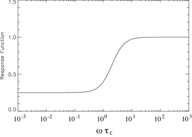
The rapidly-perturbed system has relaxation response over a timescale $\tau_{c}$, as can be seen from the response function in frequency. Fourier transforming eqs. (14) and (15), and eliminating the Fourier transform of $\Omega_{f}(t)$, gives

$$\left|\tilde{\Omega}_{c}(\omega)\right|^{2}=\frac{1}{\omega^{2}I_{c}^{2}}\left[\frac{(\omega\tau_{c})^{2}+(I_{c}/I_{f})^{2}}{(\omega\tau_{c})^{2}+(I/I_{f})^{2}}\right]\left|\tilde{N}(\omega)\right|^{2};$$ (18)

We define the response function as the frequency dependent term in brackets, shown in Fig. 10. At frequencies higher than $\omega\tau_{c}=1$, only the crust responds to the torque. At lower frequencies, the entire moment of inertia of the star $I$ is perturbed by the torque, resulting in a lower response. There is a “knee” in the spectrum at $\omega\tau_{c}\simeq 1$. Such a knee is evident in the power spectrum of the simulated phase residuals (Fig. 9 - top right panel).

Figure 10: Frequency dependent response function of the crust in the two-component model, normalized to unity. The knee at $\omega\tau_{c}$ represents the transition from coupled to decoupled response.

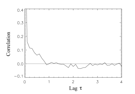
In Fig. 9 (bottom panels), we have added gaussian noise to the time series to simulate noisy data. In this case, the knee in the spectrum corresponding to the coupling timescale $\tau_{c}$ becomes buried beneath the noise. Time domain analysis is better suited for this noise-dominated time series. We calculate the autocorrelation function of the time series shown in Fig. 9 (bottom left). The coupling time is readily seen in the autocorrelation function shown in Fig. 11.

Figure 11: The autocorrelation function for the simulated time series shown in Fig. 9 (bottom left panel), showing the intrinsic relaxation time of the system that is not visible in the power spectrum.

A.3 DCF Tests

Figure 12: Top - Schematic of the sawtooth function. Each impulse decays linearly over a timescale of 10 units. Impulses are randomly spaced in time, with random amplitudes of either sign drawn from a Gaussian distribution with a standard deviation of unity. Bottom - Simulated residuals consisting of periodic functions, a polynomial, Gaussian noise, and a sawtooth function. Several gaps are added to simulate the sampling we have for the real data. The effects of the sawtooth function are too small to be seen against the wander and added noise.

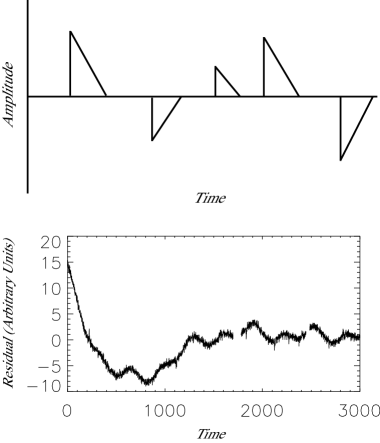
To illustrate that the DCF can distinguish between correlations due to wander and those due to a relaxation process, we add a series of 10 “sawtooth” functions to the synthetic data of Fig. 9 (lower panel). Each sawtooth consists of a discontinuous jump of random magnitude, followed by a linear decay over 10 time units. The jumps are randomly spaced over the time series, with magnitudes drawn from a Gaussian with a standard deviation of unity about zero; see Fig. 12 (top panel). The resulting data are shown in Fig. 12 (bottom panel); the effects of the sawtooth are too small to be seen in these simulated data. We have also added gaps to simulate real data. We show data with even sampling (apart from the gaps); we have confirmed that uneven sampling has a negligible effect on the results.

Figure 13: DCFs for whitened simulated residuals using $W=75,50,25$, after adding a “sawtooth” function to the simulated residuals shown in Fig. 12. The relaxation timescale of 10 units is easily identified for $W=75$, with low-frequency wander nearly completely subtracted by the high-pass filter. For $W=50$, the fitting function begins to subtract the correlations. At $W=25$, the time series is overwhitened, resulting in reduction of the relaxation signature and anticorrelations from lags in the range $5\lesssim\tau\lesssim 25$.

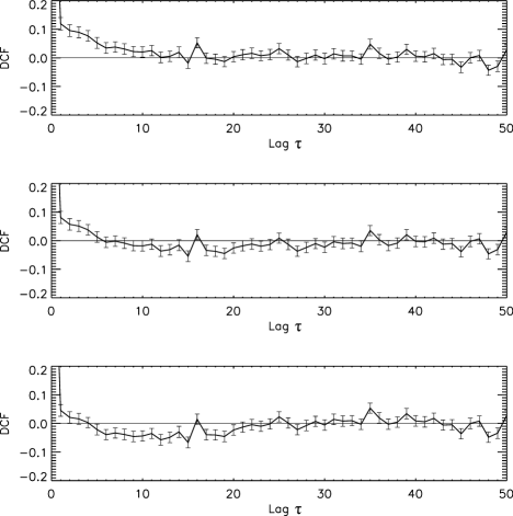
DCFs for this time series upon whitening are shown in Fig. 13 for three filter widths $W$. For $W=75$, only positive correlations over $\sim 10$ time units are evident (top panel), as the low-frequency wander has been almost completely subtracted. This DCF signature is easily differentiated from the variability arising from the impulsive noise, which produces both correlations and anti-correlations. At lower values of $W$, the fitting function begins to remove correlations in the data, and anti-correlations begin to appear (middle and bottom panels); these data have been overwhitened. For a broad range in $W$, correlations remain evident, even if the data have been overwhitened.

The LD for the synthetic data of Fig. 12 (bottom panel) is shown in Fig. 14. We decorrelated the data through random shuffling of the points. For 100 such shufflings, we calculated the average ${\rm LD}(\tau)$ to establish the base ${\rm LD}(\tau)$ one would expect under the null hypothesis that the data are completely uncorrelated. These values are shown as the horizontal lines in each figure; ${\rm LD}(\tau)$ is normalized in terms of this average value. This method has the advantage that nothing is assumed about the underlying statistics of the data, rather, the data themselves are used to evaluate ${\rm LD}(\tau)$ for the null hypothesis. Uncertainties are calculated using eq. 7. The LD shows that the data are correlated over a timescale of 10 time units, consistent with results of the DCF for this simulated time series (Fig. 13).

We conclude that high-pass filtering of the time series followed by calculation of the DCF is a robust method for identifying an intrinsic relaxation timescale $\tau_{c}$, provided the following conditions are met:

$$\Delta t_{\rm samp}<\tau_{c}<\tau_{\rm wander},$$ (19)

where $\Delta t_{\rm samp}$ is the mean sampling interval and $\tau_{\rm wander}$ is the shortest timescale of the wander. If the first inequality is not satisfied, then the time resolution of the data is not sufficient to resolve the correlation timescale. If the second condition is not met, then the correlation cannot be disentangled from the wander. In practice, we must also require

$$\tau_{\rm corr}<W<\tau_{\rm wander},$$ (20)

to ensure that the filter removes the wander but not the correlation. In the extreme case of $W\sim\tau_{\rm samp}$, the filtering method introduces spurious anti-correlations, indicating that $W$ is too small.

Figure 14: LD of the simulated time series shown in Fig. 12, after whitening with $W=75$. The relaxation process occurring over 10 time units is evident, confirming the results of the DCF shown in Fig. 13.

A.4 Robustness Tests

Figure 15: DCF for PSR B1133+16, using three different whitening methods. In the top panel, the whitening method described in Section 2.1 is used with $W=400$ d. (For other values of $W$, see Fig. 16). For the middle panel, timing residuals were whitened using a fifth-order polynomial. For the bottom panel, the DCF function itself was whitened using $W=400$ d (see text).

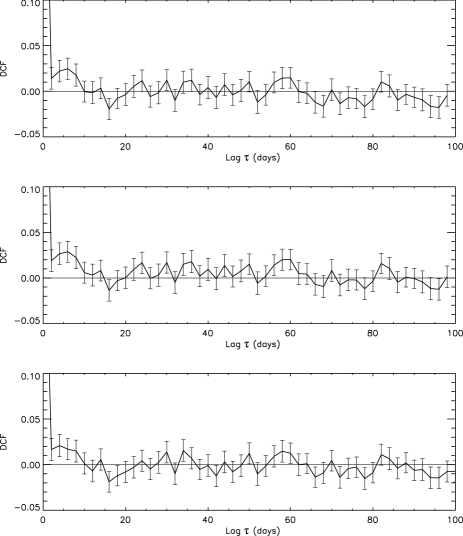
To verify that the correlations found using the DCF are not introduced by the whitening method, we compare our results to those found using other whitening methods, using data from PSR B1133+16 for illustration. The wander in this pulsar can be adequately removed with a fifth-order polynomial. Applying the DCF analysis to the data whitened using this technique, the results are very similar to those we find using the technique described in Section 2.1 (Fig. 15 middle panel). We also apply the DCF to unwhitened data for PSR B1133+16, and then whiten the correlation function, rather than the time series, to remove the signature of low-frequency wander from the DCF (Fig. 15, bottom panel). These three whitening techniques give very similar results.

Figure 16: DCFs for PSR B1133+16 (left column) and PSR B1933+16 (right column) for several values of $W$. For B1133+16, the top panel uses $W=600$ days, the middle panel uses $W=200$ days, and the bottom panel uses $W=80$ days. In the range $W\sim 100-500$ days, the DCFs are nearly indistinguishable. For B1933+16, the top panel uses $W=140$ days, the middle panel uses $W=100$ days, and the bottom panel uses $W=60$ days. For $W\sim 80-120$ days, the DCFs are similar and show correlations for $\tau\lesssim 30$ d.

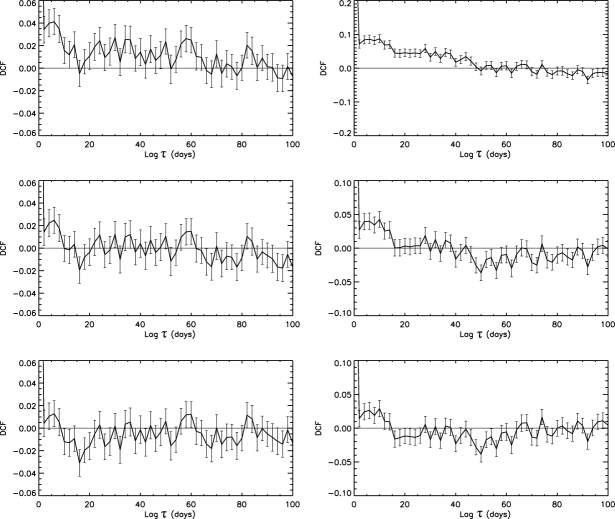
For B1133+16, the large difference between the relaxation timescale ($\sim 10$ d) and the wander timescale ($\sim 1000$ d) allows a wide range of choices for the high-pass filter width $W$ that give similar results. The wander is not well removed for $W\gtrsim 600$ days, and the fitting function begins to subtract the relaxation correlations for $W\lesssim 100$ days. We show DCFs for PSR B1133+16 for several values of $W$ in Fig. 16 (left column).

The characteristic timescale of the wander is much shorter for B1933+16, about 300 d. We plot several DCFS for B1933+16 for different values of $W$ (Fig. 16, right column). To successfully remove the wander, $W$ must be a factor of several smaller than the shortest characteristic timescales of the wander. We also ensure that $W$ is a factor of 2-3 greater than the relaxation timescale that appears in the DCF as $W$ is reduced. In the case of B1933+16, these constraints leave little room to vary $W$. For $W\sim 80-120$ days, the DCFs are nearly identical. For Figs. 2 and 3, we use a cutoff frequency of $f\sim 400$ d^-1 for B1133+16, and $f\sim 120$ d^-1 for B1933+16.

References

- Alpar et al. (1984) Alpar M. A., Anderson P. W., Pines D., Shaham J., 1984, Astrophys. J., 276, 325
- Alpar et al. (1986) Alpar M. A., Nandkumar R., Pines D., 1986, Astrophys. J., 311, 197
- Boynton (1981) Boynton P. E., 1981, in Wielebinski R., Sieber W., eds, IAU Symposium No. 95, Pulsars Reidel, Dordrecht, p. 279
- Boynton & Deeter (1979) Boynton P. E., Deeter J. E., 1979, in Lamb F. K., Pines D., eds, Compact Galactic X-ray Sources. University of Illinois, Urbana, p. 168
- Boynton et al. (1984) Boynton P. E., Deeter J. E., Lamb F. K., Zylstra G., Pravdo S. H., White N. E., Wood K. S., Yentis D. J., 1984, Astrophys. J., 283, L53
- Boynton et al. (1972) Boynton P. E., Groth E. J., Hutchinson D. P., Nanos G. P., Jr R. B. P., Wilkinson D. T., 1972, Astrophys. J., 175, 217
- Cheng (1987a) Cheng K. S., 1987a, Astrophys. J., 321, 799
- Cheng (1987b) Cheng K. S., 1987b, Astrophys. J., 321, 805
- Cordes (1980) Cordes J. M., 1980, Astrophys. J., 237, 216
- Cordes (1993) Cordes J. M., 1993, in Phillips J. A., Thorsett J. E., Kulkarni S. R., eds, Planets Around Pulsars Vol. 36. Astronomical Society of the Pacific Conference Series, San Francisco, CA, p. 43
- Cordes & Downs (1985) Cordes J. M., Downs G. S., 1985, Astrophys. J. Suppl. S., 59, 343
- Edelson & Krolik (1988) Edelson R. A., Krolik J. H., 1988, Astrophys. J., 333, 646
- Fukumura et al. (2010) Fukumura K., Shrader C. R., Dong J. W., Kazanas D., 2010, Astron. Astrophys., 524, A34
- Hobbs et al. (2010) Hobbs G., Lyne A. G., Kramer M., 2010, Mon. Not. R. Astron. Soc., 402, 1027
- Hobbs et al. (2004) Hobbs G., Lyne A. G., Kramer M., Martin C. E., Jordan C., 2004, Mon. Not. R. Astron. Soc., 353, 1311
- Hobbs et al. (2006) Hobbs G. B., Edwards R. T., Manchester R. N., 2006, MNRAS, 369, 655
- Jones (1990) Jones P. B., 1990, Mon. Not. Roy. Astr. Soc., 246, 364
- Lamb et al. (1978) Lamb F. K., Pines D., Shaham J., 1978, Astrophys. J., 225, 582
- Link et al. (1993) Link B., Epstein R. I., Baym G., 1993, Astrophys. J., 403, 285
- Liu et al. (2011) Liu K., Verbiest J. P. W., Kramer M., Stappers B. W., van Straten W., Cordes J. M., 2011, Mon. Not. R. Astron. Soc., 417, 2916
- Lyne et al. (2010) Lyne A., Hobbs G., Kramer M., Stairs I., Stappers B., 2010, Science, 329, 408
- Lyne & Graham-Smith (2005) Lyne A. G., Graham-Smith F., 2005, Pulsar Astronomy. Cambridge University Press
- Lyne et al. (2000) Lyne A. G., Shemar S. L., Smith F. G., 2000, Mon. Not. Roy. Astr. Soc., 315, 534
- Pizzochero (2011) Pizzochero P. M., 2011, Astrophys. J., 743, L20
- Rickett (1990) Rickett B. J., 1990, Ann. Rev. Astron. Astrophys., 28, 561
- Shabanova & Shitov (2004) Shabanova T. V., Shitov Y. P., 2004, Astron. Astrophys., 418, 203
- Stinebring et al. (1992) Stinebring D. R., Kaspi V. M., Nice D. J., Ryba M. F., Taylor J. H., Thorsett S. E., Hankins T. H., 1992, Rev. Sci. Instr., 53, 3551
- Urama et al. (2006) Urama J. O., Link B., Weisberg J. M., 2006, Mon. Not. Roy. Astr. Soc., 370, L76
- van Haasteren et al. (2009) van Haasteren R., Levin Y., McDonald P., Lu T., 2009, Mon. Not. Roy. Astron. Soc., 395, 1005
- You et al. (2007) You X. P., Hobbs G., Coles W. A., Manchester R. N., Edwards R., Bailes M., Sarkissian J., Verbiest J. P. W., van Straten W., Hotan A., Ord S., Jenet F., Bhat N. D. R., Teoh A., 2007, MNRAS, 378, 493