Cross-conformal predictors

Abstract

This note introduces the method of cross-conformal prediction, which is a hybrid of the methods of inductive conformal prediction and cross-validation, and studies its validity and predictive efficiency empirically.

1 Introduction

The method of conformal prediction produces set predictions that are automatically valid in the sense that their unconditional coverage probability is equal to or exceeds a preset confidence level ([14], Chapter 2). A more computationally efficient method of this kind is that of inductive conformal prediction ([12], [14], Section 4.1, [1]). However, inductive conformal predictors are typically less predictively efficient, in the sense of producing larger prediction sets as compared with conformal predictors. Motivated by the method of cross-validation [11, 13], this note explores a hybrid method, which we call cross-conformal prediction.

We are mainly interested in the problems of classification and regression, in which we are given a training set consisting of examples, each example consisting of an object and a label, and asked to predict the label of a new test object; in the problem of classification labels are elements of a given finite set, and in the problem of regression labels are real numbers. If we are asked to predict labels for more than one test objects, the same prediction procedure can be applied to each test object separately. In this introductory section and in our empirical studies we consider the problem of binary classification, in which labels can take only two values, which we will encode as 0 and 1. We always assume that the examples (both the training examples and the test examples, consisting of given objects and unknown labels) are generated independently from the same probability measure; this assumption will be called the assumption of randomness.

The idea of conformal prediction is to try the two different labels, 0 and 1, for the test object, and for either postulated label to test the assumption of randomness by checking how well the test example conforms to the training set; the output of the procedure is the corresponding p-values $p^{0}$ and $p^{1}$. Two standard ways to package the pair $(p_{0},p_{1})$ are:

• Report the confidence $1-\min(p^{0},p^{1})$ and credibility $\max(p^{0},p^{1})$.

• For a given significance level $\epsilon\in(0,1)$ output the corresponding prediction set $\{y\mid p^{y}>\epsilon\}$.

In inductive conformal prediction the training set is split into two parts, the proper training set and the calibration set. The two p-values $p^{0}$ and $p^{1}$ are computed by checking how well the test example conforms to the calibration set. The way of checking conformity is based on a prediction rule found from the proper training set and produces, for each example in the calibration set and for the test example, the corresponding “conformity score”. The conformity score of the test example is then calibrated to the conformity scores of the calibration set to obtain the p-value. For details, see Section 2.

Inductive conformal predictors are usually much more computationally efficient than the corresponding conformal predictors. However, they are less predictively efficient: they use only the proper training set when developing the prediction rule and only the calibration set when calibrating the conformity score of the test example, whereas conformal predictors use the full training set for both purposes.

Cross-conformal prediction modifies inductive conformal prediction in order to use the full training set for calibration and significant parts of the training set (such as $80\%$ or $90\%$) for developing prediction rules. The training set is split into $K$ folds of equal (or almost equal) size. For each $k=1,\ldots,K$ we construct a separate inductive conformal predictor using the $k$th fold as the calibration set and the rest of the training set as the proper training set. Let $(p^{0}_{k},p^{1}_{k})$ be the corresponding p-values. Next the two sets of p-values, $p^{0}_{k}$ and $p^{1}_{k}$, are merged into combined p-values $p^{0}$ and $p^{1}$, which are the result of the procedure.

In Appendix A we consider the most standard way of combining p-values, Fisher’s method. However, the method produces badly miscalibrated results as it assumes the independence of the p-values being combined, whereas in fact these p-values are heavily dependent. In the main part of the note, namely in Section 3, we, essentially, combine p-values by averaging them. This leads to much better calibration; since we have no theoretical results about the validity of cross-conformal prediction in this note, we rely on empirical studies involving the standard Spambase data set. Finally, we use the same data set to demonstrate the efficiency of cross-conformal predictors as compared with inductive conformal predictors. Section 4 states an open problem.

2 Inductive conformal predictors

We fix two measurable spaces: $\mathbf{X}$, called the object space, and $\mathbf{Y}$, called the label space. The Cartesian product $\mathbf{Z}:=\mathbf{X}\times\mathbf{Y}$ is the example space. A training set is a sequence $(z_{1},\ldots,z_{l})\in\mathbf{Z}^{l}$ of examples $z_{i}=(x_{i},y_{i})$, where $x_{i}\in\mathbf{X}$ are the objects and $y_{i}\in\mathbf{Y}$ are the labels. For $S\subseteq\{1,\ldots,l\}$, we let $z_{S}$ stand for the sequence $(z_{s_{1}},\ldots,z_{s_{n}})$, where $s_{1},\ldots,s_{n}$ is the sequence of all elements of $S$ listed in the increasing order (so that $n:=\left|S\right|$).

In the method of inductive conformal prediction, we split the training set into two non-empty parts, the proper training set $z_{T}$ and the calibration set $z_{C}$, where $(T,C)$ is a partition of $\{1,\ldots,l\}$. An inductive conformity measure is a measurable function $A:\mathbf{Z}^{*}\times\mathbf{Z}\to\mathbb{R}$ (we are interested in the case where $A(\zeta,z)$ does not depend on the order of the elements of $\zeta\in\mathbf{Z}^{*}$). The idea behind the conformity score $A(z_{T},z)$ is that it should measure how well the example $z$ conforms to the proper training set $z_{T}$. A standard choice is

$$A(z_{T},(x,y)):=\Delta(y,f(x)),$$ (1)

where $f:\mathbf{X}\to\mathbf{Y}^{\prime}$ is a prediction rule found from $z_{T}$ as the training set and $\Delta:\mathbf{Y}\times\mathbf{Y}^{\prime}\to\mathbb{R}$ is a measure of similarity between a label and a prediction. Allowing $\mathbf{Y}^{\prime}$ to be different from $\mathbf{Y}$ (usually $\mathbf{Y}^{\prime}\supset\mathbf{Y}$) may be useful when the underlying prediction method gives additional information to the predicted label; e.g., the MART procedure used in Section 3 and Appendix A gives the logit of the predicted probability that the label is $1$.

The inductive conformal predictor (ICP) corresponding to $A$ is defined as the set predictor

$$\Gamma^{\epsilon}(z_{1},\ldots,z_{l},x):=\{y\mid p^{y}>\epsilon\},$$ (2)

where $\epsilon\in(0,1)$ is the chosen significance level ($1-\epsilon$ is known as the confidence level), the p-values $p^{y}$, $y\in\mathbf{Y}$, are defined by

$$p^{y}:=\frac{\left|\left\{i\in C\mid\alpha_{i}\leq\alpha^{y}\right\}\right|+1}{\left|C\right|+1},$$

and

$$\alpha_{i}:=A(z_{T},z_{i}),\quad i\in C,\qquad\alpha^{y}:=A(z_{T},(x,y))$$ (3)

are the conformity scores. Given the training set and a test object $x$ the ICP predicts its label $y$; it makes an error if $y\notin\Gamma^{\epsilon}(z_{1},\ldots,z_{l},x)$.

The random variables whose realizations are $x_{i}$, $y_{i}$, $z_{i}$, $x$, $y$, $z$ will be denoted by the corresponding upper case letters ($X_{i}$, $Y_{i}$, $Z_{i}$, $X$, $Y$, $Z$, respectively). The following proposition of validity is almost obvious.

Proposition 1 ([14], Proposition 4.1).

If random examples $Z_{1},\ldots,Z_{l},$ $Z=(X,Y)$ are i.i.d., the probability of error $Y\notin\Gamma^{\epsilon}(Z_{1},\ldots,Z_{l},X)$ does not exceed $\epsilon$ for any $\epsilon$ and any inductive conformal predictor $\Gamma$.

The family of prediction sets $\Gamma^{\epsilon}(z_{1},\ldots,z_{l},x)$, $\epsilon\in(0,1)$, is just one possible way of packaging the p-values $p^{y}$. Another way, already discussed in Section 1 in the context of binary classification, is as the confidence $1-p$, where $p$ is the second largest p-value among $p^{y}$, and the credibility $\max_{y}p^{y}$. In the case of binary classification confidence and credibility carry the same information as the full set $\{p^{y}\mid y\in\mathbf{Y}\}$ of p-values, but this is not true in general.

In our experiments reported in the next section we split the training set into the proper training set and the calibration set in proportion $2:1$. This is the most standard proportion (cf. [9], p. 222, where the validation set plays a similar role to our calibration set), but the ideal proportion depends on the learning curve for the given problem of prediction (cf. [9], Figure 7.8). Too small a calibration set leads to a high variance of confidence (since calibrating conformity scores becomes unreliable) and too small a proper training set leads to a downward bias in confidence (conformity scores based on a small proper training set cannot produce confident predictions). In the next section we will see that using cross-conformal predictors improves both bias and variance (cf. Table 1).

3 Cross-conformal predictors

Cross-conformal predictors (CCP) are defined as follows. The training set is split into $K$ non-empty subsets (folds) $z_{S_{k}}$, $k=1,\ldots,K$, where $K\in\{2,3,\ldots\}$ is a parameter of the algorithm and $(S_{1},\ldots,S_{K})$ is a partition of $\{1,\ldots,l\}$. For each $k\in\{1,\ldots,K\}$ and each potential label $y\in\mathbf{Y}$ of $x$ find the conformity scores of the examples in $z_{S_{k}}$ and of $(x,y)$ by

$$\alpha_{i,k}:=A(z_{S_{-k}},z_{i}),\quad i\in S_{k},\qquad\alpha^{y}_{k}:=A(z_{S_{-k}},(x,y)),$$ (4)

where $S_{-k}:=\cup_{j\neq k}S_{j}$ and $A$ is a given inductive conformity measure. The corresponding p-values are defined by

$$p^{y}:=\frac{\sum_{k=1}^{K}\left|\left\{i\in S_{k}\mid\alpha_{i,k}\leq\alpha^{y}_{k}\right\}\right|+1}{l+1}.$$ (5)

Confidence and credibility are now defined as before; the set predictor $\Gamma^{\epsilon}$ is also defined as before, by (2), where $\epsilon>0$ is another parameter.

The definition of CCPs parallels that of ICPs, except that we now use the whole training set for calibration. The conformity scores (4) are computed as in (3) but using the union of all the folds except for the current one as the proper training set. Calibration (5) is done by combining the ranks of the test example $(x,y)$ with a postulated label in all the folds.

If we define the separate p-value

$$p^{y}_{k}:=\frac{\left|\left\{i\in S_{k}\mid\alpha_{i,k}\leq\alpha^{y}_{k}\right\}\right|+1}{\left|S_{k}\right|+1}$$ (6)

for each fold, we can see that $p^{y}$ is essentially the average of $p^{y}_{k}$. In particular, if each fold has the same size, $\left|S_{1}\right|=\cdots=\left|S_{K}\right|$, a simple calculation gives

$$p^{y}=\bar{p}^{y}+\frac{K-1}{l+1}\left(\bar{p}^{y}-1\right)\approx\bar{p}^{y},$$ (7)

where $\bar{p}^{y}:=\frac{1}{K}\sum_{k=1}^{K}p^{y}_{k}$ is the arithmetic mean of $p^{y}_{k}$ and the $\approx$ assumes $K\ll l$.

In this note we give calibration plots for 5-fold and 10-fold cross-conformal prediction. We take $K\in\{5,10\}$ following the advice in [9] (who refer to Breiman and Spector [3] and Kohavi [10]). In our experiments we use the popular Spambase data set. The size of the data set is 4601, and there are two labels: spam, encoded as 1, and email, encoded as 0.

We consider the conformity measure (1) where $f$ is output by MART ([9], Chapter 10) and

$$\Delta(y,f(x)):=\begin{cases}f(x)&\text{if $y=1$}\\ -f(x)&\text{if $y=0$}.\end{cases}$$ (8)

MART’s output $f(x)$ models the log-odds of spam vs email,

$$f(x)=\log\frac{P(1\mid x)}{P(0\mid x)},$$

which makes the interpretation of (8) as conformity score very natural. (MART is known [9] to give good results on the Spambase dataset.)

The R programs used in the experiments described in this section and the appendix have been uploaded to arXiv. The programs use the gbm package with virtually all parameters set to the default values (given in the description provided in response to help("gbm")). The only parameter that has been modified is n.trees, the number of trees, which should be as large as possible and whose default value was clearly insufficient.

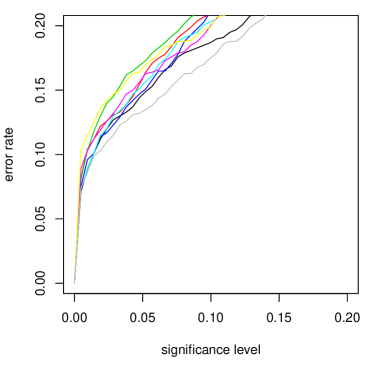
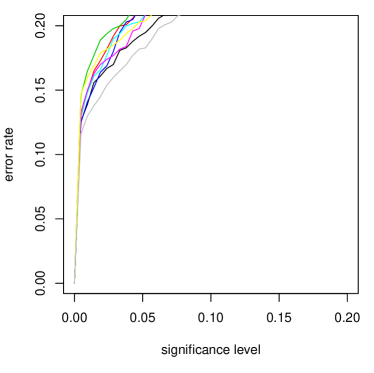
Figure 1 gives the calibration plots for the CCP and for 8 random splits of the data set into a training set of size 3600 and a test set of size 1001 and of the training set into 5 or 10 folds. There is a further source of randomness as the MART procedure is itself randomized. The functions plotted in Figure 1 map each significance level $\epsilon$ to the percentage of erroneous predictions made by the set predictor $\Gamma^{\epsilon}$ on the test set. Visually, the plots are well-calibrated (close to the bisector of the first quadrant).

Figure 1: Left panels: the calibration plot for the cross-conformal predictor with $K=5$ (top) and $K=10$ (bottom) folds and the first 8 seeds, 0–7, for the R pseudorandom number generator. Right panels: the lower left corner of the corresponding left panel (which is the most important part of the calibration plot in applications).

As for the efficiency of the CCP, see Table 1. The biggest advantage of the CCP is in the stability of its confidence values: the standard deviation of the mean confidences is much less than that for the ICP. However, the CCP also gives higher confidence; to some degree this can be seen from the table, but the high variance of the ICP confidence masks it: e.g., for the first 100 seeds the average of the mean confidence for ICP is $99.16\%$ (with the standard deviation of the mean confidences equal to $0.149\%$, corresponding to the standard deviation of $0.015\%$ of the average mean confidence).

Seed	0	1	2	3	4	5	6	7	Average	St. dev.
mean conf., ICP	99.25%	99.23%	99.00%	99.17%	99.30%	99.12%	99.38%	99.25%	99.21%	0.109%
mean cred., ICP	51.31%	50.37%	49.93%	52.45%	48.98%	50.34%	50.18%	52.00%	50.69%	1.074%
mean conf., $K=5$	99.22%	99.17%	99.17%	99.24%	99.27%	99.27%	99.30%	99.30%	99.24%	0.050%
mean cred., $K=5$	51.06%	49.70%	50.26%	50.63%	49.81%	49.42%	50.88%	51.40%	50.39%	0.664%
mean conf., $K=10$	99.24%	99.20%	99.20%	99.23%	99.26%	99.28%	99.34%	99.32%	99.26%	0.048%
mean cred., $K=10$	51.02%	49.69%	50.23%	50.71%	49.70%	49.42%	50.89%	51.39%	50.38%	0.678%

Table 1: Mean (over the test set) confidence and credibility for the ICP and the 5-fold and 10-fold CCP. The results are given for various values of the seed for the R pseudorandom number generator; column “Average” gives the average of all the 8 values for the seeds 0–7, and column “St. dev.” gives the standard deviation of those 8 values.

4 Conclusion

Conformal prediction and inductive conformal prediction are two approaches to the theory of tolerance regions (see, e.g., [5]). The known validity results for conformal and inductive conformal predictors can be expressed by saying that they are $1-\epsilon$ expectation tolerance regions, where $\epsilon$ is the significance level (see Proposition 1 above for the case of ICPs). It is also known ([2], Proposition 2a) that inductive conformal predictors are $1-\delta$ tolerance regions for a proportion $1-\epsilon$ for suitable $\delta$ and $\epsilon$. On the other hand, at this time there are no theoretical results about the validity of cross-conformal predictors, and it is an interesting open problem to establish such results.

Acknowledgments

The empirical studies described in this paper used the R system and the gbm package written by Greg Ridgeway (based on the work of Freund and Schapire [6] and Friedman [7, 8]). This work was partially supported by the Cyprus Research Promotion Foundation.

Appendix A An approach based on Fisher’s method

In this appendix we will briefly discuss an approach to cross-conformal prediction leading to miscalibrated set predictions.

Fisher’s method [4] of combining p-values $p_{1},\ldots,p_{K}$, valid when the $K$ p-values are independent, combines them into one statistic $-2\sum_{k=1}^{K}\ln p_{k}$ having the chi-squared distribution with $2K$ degrees of freedom. The corresponding p-value will be denoted $F(p_{1},\ldots,p_{K})$:

$$F(p_{1},\ldots,p_{K}):=\operatorname{\mathbb{P}}\left(\chi^{2}\geq-2\sum_{k=1}^{K}\ln p_{k}\right),$$ (9)

where $\chi^{2}$ is a random variable having the chi-squared distribution with $2K$ degrees of freedom.

Naive cross-conformal predictors are defined as follows. The training set is split into $K$ subsets, as in the case of CCPs. For each $k\in\{1,\ldots,K\}$ find the p-values $p^{y}_{k}$ via (6). Define $p^{y}:=F(p^{y}_{1},\ldots,p^{y}_{K})$, and then define confidence, credibility, and set predictors (2) as before. In other words, naive cross-conformal predictors are defined in the same way as cross-conformal predictors except that the function $F$ is defined by (9) rather than by the expression following the $=$ in (7).

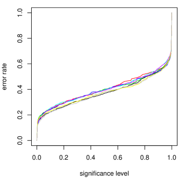
Figure 2 is the analogue of Figure 1 for naive cross-conformal predictors. It is obvious that the set predictions are badly miscalibrated; the p-values computed from different folds are heavily dependent. This may appear counterintuitive, but the reader should remember that we are dealing with a somewhat unusual kind of hypothesis testing in this note (and in the theory of tolerance regions in general): instead of testing some properties of the data-generating distribution we are testing hypotheses about data.

We do not give the efficiency results (such as those given in Table 1) for the naive CCP since efficiency without validity is meaningless.

Figure 2: The analogue of Figure 1 for the naive cross-conformal predictor.

References

- [1] Anonymous. Generalized conformal prediction for functional data. Submitted to NIPS 2012, June 2012.
- [2] Anonymous. Inductive conformal predictors in the batch mode. Submitted to ACML 2012, July 2012.
- [3] Leo Breiman and Philip Spector. Submodel selection and evaluation in regression: the -random case. International Statistical Review, 60:291–319, 1992.
- [4] Ronald A. Fisher. Combining independent tests of significance. American Statistician, 2:30, 1948. This is the answer to Question 14 in Frederick Mosteller’s “Questions and Answers” column.
- [5] Donald A. S. Fraser. Nonparametric Methods in Statistics. Wiley, New York, 1957.
- [6] Yoav Freund and Robert E. Schapire. A decision-theoretic generalization of on-line learning and an application to boosting. Journal of Computer and System Sciences, 55:119–139, 1997.
- [7] Jerome H. Friedman. Greedy function approximation: A gradient boosting machine. Annals of Statistics, 29:1189–1232, 2001.
- [8] Jerome H. Friedman. Stochastic gradient boosting. Computational Statistics and Data Analysis, 38:367–378, 2002.
- [9] Trevor Hastie, Robert Tibshirani, and Jerome Friedman. The Elements of Statistical Learning: Data Mining, Inference, and Prediction. Springer, New York, second edition, 2009.
- [10] Ron Kohavi. A study of cross-validation and bootstrap for accuracy estimation and model selection. In Proceedings of the International Joint Conference on Artificial Intelligence (IJCAI), pages 1137–1143. Morgan Kaufmann, 1995.
- [11] Frederick Mosteller and John W. Tukey. Data analysis, including statistics. In G. Lindzey and E. Aronson, editors, Handbook of Social Psychology, volume 2, pages 80–203. Addison-Wesley, Reading, MA, second edition, 1968.
- [12] Harris Papadopoulos, Vladimir Vovk, and Alex Gammerman. Qualified predictions for large data sets in the case of pattern recognition. In Proceedings of the First International Conference on Machine Learning and Applications (ICMLA), pages 159–163, Las Vegas, NV, 2002. CSREA Press.
- [13] Mervin Stone. Cross-validatory choice and assessment of statistical predictions (with discussion). Journal of the Royal Statistical Society Series B, 36:111–147, 1974.
- [14] Vladimir Vovk, Alex Gammerman, and Glenn Shafer. Algorithmic Learning in a Random World. Springer, New York, 2005.