Abstract: Resource-based competition between microorganisms species in continuous culture has been studied extensively both experimentally and theoretically, mostly for bacteria through Monod and and Contois "constant yield" models, or for phytoplankton through the Droop "variable yield” models. For homogeneous populations of N bacterial species (Monod) or N phytoplanktonic species (Droop), with one limiting substrate and under constant controls, the theoretical studies [1, 2, 3] indicated that competitive exclusion occurs: only one species wins the competition and displaces all the others. The winning species expected from theory is the one with the lowest "substrate subsistence concentration" $s^{\star}$, such that its corresponding equilibrium growth rate is equal to the dilution rate $D$. This theoretical result was validated experimentally with phytoplankton [4] and bacteria [5], and observed in a lake with microalgae [6]. On the contrary for attached bacterial species described by a Contois model, theory [7] predicts coexistence between several species. In this paper we present a generalization of these results by studying a competition between three different types of microorganisms : free bacteria (represented by a generalized Monod mode), attached bacteria (represented by a Contois model) and free phytoplankton (represented by a Droop model). We prove that the outcome of the competition is a coexistence between several attached bacterial species with a free species of bacteria or phytoplankton, all the other free species being washed out. This demonstration is based mainly on the study of the substrate concentration’s evolution caused by competition; it converges towards the lowest subsistence concentration $s^{\star}$, leading to three different types of competition outcome: 1. only the free bacteria/ phytoplankton best competitor excludes all other species; 2. only some attached bacterial species coexist in the chemostat; 3. A coexistence between the best free species, with one or several attached species.

Key-words: competition, competitive exclusion, droop, variable yield model, monod, ratio-dependent, biomass-dependent, microorganism, microalgae, phytoplankton

Competition entre phytoplankton et bacteries: exclusion et coexistence

Résumé : La comp tition pour la ressource entre micro-organismes dans des cultures en continu a t largement tudi e exp rimentalement et th oriquement, surtout entre bact ries mod lis es par des taux de croissance de type Monod ou Contois, ou pour le phytoplancton travers le mod le de Droop. Pour les populations homog nes compos es de N esp ces bact riennes (Monod) ou N esp ces phytoplanctoniques (Droop), avec un substrat limitant et des commandes maintenues constantes, les tudes th oriques [1, 2, 3] ont indiqu que l’exclusion comp titive se produit: une seul esp ce remporte la comp tition et limine toutes les autres. L’esp ce dont la th orie pr dit la victoire est celle avec la concentration $s^{\star}$ de substrat permettant sa survie la plus basse. Ce r sultat th orique a t valid e exp rimentalement pour le phytoplancton [4] et les bact ries [5], et a été observ dans un lac avec des microalgues [6]. Par contre, pour les esp ces bact riennes d crites par un mod le Contois, la th orie pr dit la coexistence entre plusieurs esp ces [7]. Dans cet article nous pr sentons une g n ralisation de ces r sultats en tudiant une compétition entre les trois diff rents types de micro-organismes: des bact ries libres (repr sent es par un mod le de Monod g n ralis ), des bact ries fix es (repr sent es par un mod le de Contois) et du phytoplancton (repr sent par un mod le de Droop). Nous prouvons que le r sultat de la comp tition est une coexistence entre plusieurs esp ces bact riennes fix es avec une esp ce de bact ries libres ou de phytoplancton, toutes les autres esp ces libres tant lessiv es. Notre d monstration est bas e principalement sur l’ tude de l’ volution du substrat caus e par la comp tition; elle converge vers la plus faible concentration de subsistance $s^{\star}$, ce qui conduit trois types diff rents des r sultats de la comp tition: 1. seule la meilleur bact rie libre ou le meilleur phytoplancton exclut toutes les autres esp ces; 2. seules quelques esp ces bact riennes fix es coexistent dans le chemostat, 3. une coexistence entre la meilleure esp ce libre, avec une ou plusieurs esp ces fix es.

Mots-clés : competition,exclusion compétitive, droop, monod, ratio-d pendence, microorganisme, microalgues, phytoplancton

1 Introduction

1.1 Growth of phytoplankton

Phytoplankton is composed of microscopic plants at the basis of the aquatic trophic chains. Phytoplankton means a broad variety of species (more than 200.000) using solar light to grow through photosynthesis. Phytoplankton plays a crucial role in nature since it is the point from which energy and carbon enter in the food web. But it may also be used in the future for food or biofuel production, since several phytoplankton species turn out to have very interesting properties in terms of protein [8, 9] or lipid [10] content. In addition to light, phytoplankton requires nutrients for its growth. The "paradox" of phytoplantkon species coexistence was introduced by Hutchinson [11]: "The problem that is presented by the phytoplankton is essentially how it is possible for a number of species to coexist in a relatively isotropic or unstructered environment all competing for the same sort of materials". In this paper we consider this question from a theoretical viewpoint "what are the mechanisms leading to competitive exclusion or coexistence, and to what competition outcome do they lead?". But so far most of the competitions studies have assumed that only phytoplankton species were engaged in the competition. However, it is clear that such species also have to compete with the bacteria for nutrients.

In this paper, we study the competition between phytoplankton and bacteria. Phytoplankton can be accurately represented by a Droop model [12, 13, 14] which accounts for their ability to store nutrients and to uncouple uptake and growth. Bacteria are represented by simpler models. They can be of two different types, described either by a Monod type model if they live in suspension or by a contois model if they are attached to a support.

In this paper we first recall the main results available for competition of microbial species of the same class. Then we consider the problem of 3 class competition. After some mathematical preliminaries we state and demonstrate our main Theorem. A discussion concludes our paper and highlights the ecological consequences of our result.

1.2 The Competitive Exclusion Principle (CEP)

"Complete competitors cannot coexist"

This is the formulation chosen by Hardin [15] to describe the Competitive Exclusion Principle (CEP). According to him, this ambiguous wording "is least likely to hide the fact that we still do not comprehend the exact limits of the principle". But still, a more precise formulation is given: if several non-interbreeding populations "do the same thing" (they occupy the same ecological niche in Elton’s sense [16]) and if they occupy the same geographic territory, then ultimately the most competitive species will completely displace the others, which will become extinct.

Darwin was already expressing this principle when he spoke about natural selection ([17] p.71 and 102). Scriven described and analyzed his work in these words: "Darwin’s success lay in his empirical, case by case, demonstration that recognizable fitness was very often associated with survival. […] Its great commitment and its profound illumination are to be found in its application to the lengthening past, not the distant future: in the tasks of explanation, not in those of prediction" [18].

Since the work of Darwin, men have tried to apprehend the limits of the principle in different context and by different means. In the next sections we present how mathematical models have shown their appropriateness for predicting the outcome of competition, in the case of chemostat-controlled microcosms.

1.3 The chemostat, a tool for studying the CEP

"Microbial systems are good models for understanding ecological processes at all scales of biological organization, from genes to ecosystems" [19]. The chemostat is a device which enables to grow microorganisms under highly controlled conditions. It consists of an open reactor crossed by a flow of water, where nourishing nutrients are provided by the input flow, whereas both nutrients and microorganisms are evacuated by the output flow. To keep a constant volume in the vessel, these two flows are kept equal. In this paper we consider that the following conditions are imposed in the chemostat: the medium is well mixed (homogeneous); only one substrate is limiting for all the species, whose only (indirect) interaction is the substrate uptake; the environmental conditions (temperature, pH, light, …) are kept constant, and so are the dilution rate $D$, corresponding to the input/output flow of water, and the input substrate concentration $s_{in}$. Figure 1 represents such a chemostat.

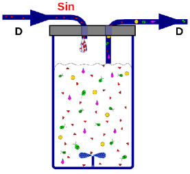
Figure 1: A chemostat, which enables to grow microorganisms under highly controlled conditions. The input/output flow of water is $D$, and the input substrate concentration is $s_{in}$

The chemostat has been used to study the CEP since the beginning of the $XX^{th}$ century [20], and its experimental use has often been coupled with mathematical models [2].

1.4 Bacterial and phytoplanktonic models, and previous theoretical results on single class competition

1.4.1 Free bacteria growth (generalized Monod model)

To predict the growth of bacteria in suspension within a chemostat, Monod developed a model [21], where the growth rates of the biomasses $x_{i}$ ($i\,\in\{1,\cdots,N_{x}\}$ for a competition between $N_{x}$ species) depend on the extracellular substrate concentration $s$. In the classical Monod model the growth rates $\alpha_{i}(s)$ are Michaelis-Menten functions

$$\alpha_{i}(s)=\frac{s}{s+K^{s}_{i}}\alpha^{m}_{i}$$

where $\alpha^{m}_{i}$ are the maximum growth rates in substrate replete conditions, and $K^{s}_{i}$ are the half saturation constants. In this paper we consider a generalized Monod model to represent growth of free bacteria, by using the wider class of functions verifying Hypothesis 1.

Hypothesis 1

M-model:
$\alpha_{i}(s)$ are $\mathcal{C}^{1}$, increasing and bounded functions such that $\alpha_{i}(0)=0$.

We note $\alpha^{m}_{i}$ the supremum of the growth rate:

$$\sup_{s\geq 0}\alpha_{i}(s)=\alpha^{m}_{i}>0$$

The free bacteria dynamics write

$$\begin{array}[]{l}\dot{x}_{i}=(\alpha_{i}(s)-D)x_{i}\\ \textrm{with }s,x_{i}\in\,{\mathbb{R}}^{+}\textrm{ for }i\,\in\{1,\cdots,N_{x}\}\textrm{ and }D\,\in{\mathbb{R}}^{+}_{*}.\end{array}$$ (1)

In this model the substrate uptake is proportional to the biomass growth for each bacterial species, so that the total substrate uptake per time unit will be $\sum_{i=1}^{N_{x}}\alpha_{i}(s)\frac{x_{i}}{a_{i}}$.

1.4.2 Phytoplankton model (generalized Droop model)

Phytoplankton is able to uncouple substrate uptake of nutrients from the growth associated to photosynthesis [13]. This capacity to store nutrients can provide a competitive advantage for the cells that can develop in situations where substrate and light (necessary for phytoplankton growth) are rarely available concomitantly. This behaviour results in varying intracellular nutrient quota: it is the proportion of assimilated substrate per unit of biomass $z_{k}$; it can be expressed for instance in mg[substrate]/mg[biomass]. Droop [12] developed a model where these internal quotas are represented by new dynamic variables $q_{k}$ (denoted "cell quota"). The substrate uptake rates $\rho_{k}(s)$ are assumed to depend on the extracellular substrate while the biomass growth rates $\gamma_{k}(q_{k})$ depend on the corresponding cell quota.

In the classical Droop model the functions have specified forms. Uptake rates are Michaelis-Menten functions (2) of the substrate concentration:

$$\rho_{k}(s)=\frac{s}{s+K^{s}_{k}}\rho^{m}_{k}$$ (2)

and the growth rates are Droop functions (3) of the cell quotas:

$$\gamma_{k}(q_{k})=\left\{\begin{array}[]{ll}\left(1-\frac{Q^{0}_{k}}{q_{k}}\right)\bar{\gamma}_{k}&\textrm{if }q_{k}\geq Q^{0}_{k}\\ 0&\textrm{if }q_{k}<Q^{0}_{k}\end{array}\right.$$ (3)

with $\rho^{m}_{k}$ and $\bar{\gamma}_{k}$ the maximal uptake and growth rates; $K^{s}_{k}$ represent the half saturation constants, and $Q^{0}_{k}$ the minimal cell quota. In this paper we consider the wider class of Q-models (Quota models) verifying Hypothesis 2, so that it can encompass, among others, the classical Droop formulation [12] as well as the Caperon-Meyer model [22].

Hypothesis 2

Q-model:

• $\rho_{k}(s)$ are $\mathcal{C}^{1}$, increasing and bounded functions such that $\rho_{k}(0)=0$

• $\gamma_{k}(q_{k})$ are $\mathcal{C}^{1}$, increasing and bounded functions for $q_{k}>Q^{0}_{k}>0$. When $q_{k}\leq Q^{0}_{k}$, $\gamma_{k}(q_{k})=0$.

It directly ensues from Hypothesis 2 that $f_{k}(q_{k})=\gamma_{k}(q_{k})q_{k}$ are increasing functions (for $q_{k}>Q^{0}_{k}$) which are onto ${\mathbb{R}}^{+}_{\star}$, so that the inverse functions $f_{k}^{-1}$ are defined on ${\mathbb{R}}^{+}_{\star}$.

We denote $\rho^{m}_{k}$ and $\bar{\gamma}_{k}$ the supremal uptake and growth rates:

$$\begin{array}[]{l}\sup_{s\geq 0}\rho_{k}(s)=\rho^{m}_{k}>0\\ \sup_{q_{k}\geq Q^{0}_{k}}\gamma_{k}(q_{k})=\bar{\gamma}_{k}>0\end{array}$$

The phytoplankton dynamics write

$$\begin{array}[]{l}\dot{q}_{k}=\rho_{k}(s)-f_{k}(q_{k})\\ \dot{z}_{k}=(\gamma_{k}(q_{k})-D)z_{k}\\ \textrm{with }s,q_{k},z_{k}\in\,{\mathbb{R}}^{+}\textrm{ for }k\,\in\{1,\cdots,N_{z}\}\textrm{ and }D\,\in{\mathbb{R}}^{+}_{*}.\par\end{array}$$ (4)

The substrate uptake per time unit is $\sum_{k=1}^{N_{z}}\rho_{k}(s)z_{k}$

This model has been experimentally shown to be better suited for phytoplankton dynamic modelling than the Monod model ([14]) that implicitly supposes that the intracellular quota is simply proportional to the substrate concentration in the medium and which must be definitely limited to bacterial modelling. The stability of the Q-model has been extensively studied in the mono-specific case ([23, 24, 25]).

1.5 Previous demonstrations of the CEP for M- and Q-models

The advantage of Monod and Droop models is that their relative simplicity allows a mathematical analysis. The analyses of the M-model with $N_{x}$ bacterial competing species [1], and of the Droop model with 2 phytoplankton species [2] and then recently with $N_{z}$ phytoplankton species [3] led to a confirmation of the CEP in the chemostat, and to a prediction on "who wins the competition", or "what criterion should a species optimize to be a good competitor". In both cases, we have

Theorem 1.1

If environmental conditions are kept constant and the competition is not controlled ($D$ and $s_{in}$ remain constant) in a chemostat, then the species with lowest "substrate subsistence concentration" $s_{i}^{x\star}$ (or $s_{k}^{z\star}$), such that its corresponding equilibrium growth rate is equal to the dilution rate $D$, is the most competitive and displaces all the others.

A striking point about this result is that it permits to make predictions on the result of a competition, only by a priori knowledge of the species substrate subsistence concentrations $s_{i}^{x\star}$ (or $s_{k}^{z\star}$). This latter can be determined in monospecific-culture chemostat, so that the competition outcome can be determined before competition really occurs. Several experimental validations where carried out with phytoplankton [4] and bacteria [5]. This theoretical behaviour was also confirmed in a lake [6], where the species with lowest phosphate or silicate subsistence concentrations won the competition for phosphate or silicate limitations.

1.5.1 Attached bacteria model (generalized Contois model)

In case where bacteria are not free in the medium but there is a spatial heterogeneity (e.g. they grow attached on a support, such as flocs in the culture medium), a ratio-dependent model is more adapted to describe bacterial growth. Contois model [26] represents such dynamics by using more complex growth functions where the growth rates depends on the ratio of the substrate concentration over biomass concentration $y_{j}$ ($j\,\in\{1,\cdots,N_{y}\}$):

$$\beta_{j}(s,y_{j})=\frac{s/y_{j}}{K^{s}_{j}+s/y_{j}}\beta^{m}_{j}$$

In this paper we consider the wider class of "C-model" (Contois model), wich is more general than a ratio dependent model. It verifies the following hypotheses:

Hypothesis 3

C-model :
$\beta_{j}(s,y_{j})$ are $\mathcal{C}^{1}$ functions on ${\mathbb{R}}^{+}\times{\mathbb{R}}^{+}\setminus\{(0,0)\}$, increasing and bounded functions of $s$ (for $y_{j}>0$), and decreasing functions of $y_{j}$ (for $s_{j}>0$) such that $\forall y_{j}\in{\mathbb{R}}^{+}_{*},\quad\beta_{j}(0,y_{j})=0$ and $\forall s\in{\mathbb{R}}^{+},\displaystyle\lim_{y_{j}\rightarrow+\infty}\beta_{j}(s,y_{j})=0$

We also need to add the following technical hyposthesis, which is verified by the classical Contois function:

Hypothesis 4

$$\frac{\partial}{\partial y_{j}}\left(\beta_{j}(s,y_{j})y_{j}\right)>0$$

We notice that the Contois growth function is undefined in $(0,0)$, and that Hypothesis 3 has been built so that this property can (but does not have to) be retained by the generalized $\beta$ function. All other properties imposed by Hypotheses 3 and 4 are satisfied by the original Contois growth-rate.

We denote $\beta^{m}_{j}(y_{j})$ the supremal growth rates for biomass concentration $y_{j}$:

$$\sup_{s\geq 0}\beta_{j}(s,y_{j})=\beta^{m}_{j}(y_{j})$$

so that the C-species dynamics write

$$\begin{array}[]{l}\dot{y}_{j}=(\beta_{j}(s,y_{j})-D)y_{j}\\ \textrm{with }s,y_{j}\in\,{\mathbb{R}}^{+}\textrm{ for }j\,\in\{1,\cdots,N_{y}\}\textrm{ and }D\,\in{\mathbb{R}}^{+}_{*}.\end{array}$$ (5)

In this model, like in the M-model, the substrate/biomass intracellular quotas $b_{j}$ are supposed to be constant for each species, so that the substrate uptake rates are proportional to the growth rates with a factor $1/b_{j}$.

1.5.2 Coexistence result for competition between C-species

Competition between several C-species was studied [7] and led to a coexistence at equilibrium with the substrate at a level $s^{y\star}$ depending on the input substrate concentration $s_{in}$ and the dilution rate $D$. The species share the available substrate. To be more precise we must define the "$s_{0}$-compliance" concept: $s_{0}$-compliant species are the species able to have a growth rate equal to the dilution rate $D$ with a substrate concentration $s_{0}$. The results of [7] show that all the "$s^{y\star}$-compliant" species coexist in the reactor at equilibirum, and all the others are washed out, as they cannot grow fast enough with substrate concentration $s^{y\star}$.

Definition 1.2

A species $x_{i},y_{j}$ or $z_{k}$ is $s_{0}$-compliant if it is able to reach a growth rate equal to the dilution rate $D$ with a substrate concentration $s_{0}$.

1.5.3 Competition and coexistence - towards a new paradigm

Following these results an interrogation arises:

$\ll$ What would be the result of a competition between "competitive" free bacterial and microalgal species, and "coexistive" attached bacterial species? Competitive exclusion? Coexistence? $\gg$

The aim of this paper is to provide an answer to this question, and to give insight into the mechanisms forcing the outcome of such a competition. This answer leads to a broader view and understanding of competitive exclusion and coexistence mechanisms, following the words of Hardin [15]: "To assert the truth of the competitive exclusion principle is not to say that nature is and always must be, everywhere,"red in tooth and claw." Rather, it is to point out that every instance of apparent coexistence must be accounted for. Out of the study of all such instances will come a fuller knowledge of the many prosthetic devices of coexistence, each with its own costs and its own benefits."

1.6 A generalized model for competition between several phytoplankton and bacteria species growing according to different kinetic models

The generalized model for competition between all bacteria and phytoplankton species is an aggregation of these models, which alltogether give the following substrate dynamics, subject to substrate input, output, and uptake rates:

$$\dot{s}=D(s_{in}-s)-\sum_{i=1}^{N_{x}}\alpha_{i}(s)\frac{x_{i}}{a_{i}}-\sum_{j=1}^{N_{y}}\beta_{j}(s,y_{j})\frac{y_{j}}{b_{j}}-\sum_{k=1}^{N_{z}}\rho_{k}(s)z_{k}$$ (6)

The parameters related to the nutrient flow are the dilution rate $D>0$ and the input substrate concentration $s_{in}>0$, which are both assumed to be constant.

To simplify notations we can remark that this system can be normalized with $a_{i}=b_{j}=1$, when considering the change of variables $\tilde{x}_{i}=\frac{x_{i}}{a_{i}}$ and $\tilde{y}_{j}=\frac{y_{j}}{b_{j}}$ (note that all the hypotheses are still satisfied). We obtain system (7) where variables $x_{i}$ and $y_{j}$ are now expressed in substrate units.

$$\begin{array}[]{l}\left\{\begin{split}\dot{s}&=D(s_{in}-s)-\sum_{i=1}^{N_{x}}\alpha_{i}(s)x_{i}-\sum_{j=1}^{N_{y}}\beta_{j}(s,y_{j})y_{j}-\sum_{k=1}^{N_{z}}\rho_{k}(s)z_{k}\\ \dot{x}_{i}&=(\alpha_{i}(s)-D)x_{i}\\ \dot{y}_{j}&=(\beta_{j}(s,y_{j})-D)y_{j}\\ \dot{z}_{k}&=(\gamma_{k}(q_{k})-D)z_{k}\\ \dot{q}_{k}&=\rho_{k}(s)-f_{k}(q_{k})\end{split}\right.\\ \textrm{with }\quad f_{k}(q_{k})=\gamma_{k}(q_{k})q_{k}\\ \textrm{and }s,q_{k}\in\,{\mathbb{R}}^{+},\quad s_{in},D\,\in{\mathbb{R}}^{+}_{*}.\textrm{and }x_{i}(0),y_{j}(0),z_{k}(0)\in\,{\mathbb{R}}^{+}_{*}\textrm{ for }i\in\{1,\cdots,N_{x}\},\\ j\in\{1,\cdots,N_{y}\},k\in\{1,\cdots,N_{z}\}\\ \end{array}$$ (7)

Note that the results obtained in this paper apply also on the simple M- only, Q-only, and C-only competition models, or on a model with two of these three kind of species.

1.7 Other coexistence mechanisms, and competition control

This introduction wouldn’t be complete without a short review of what has been done concerning other coexistive models, or the control of competition.

Following the question arised by Hutchinson [11] concerning the "paradox of the phytoplankton", a large amount of work has been done to explore the mechanisms that enable coexistence, mainly for models derived from the Monod model. It has been shown to occur in multi-resource models [27, 28], in case of non instantaneous growth [29], in some turbidity operating conditions [30], a crowding effect [31], or variable yield [32] (not in the Droop sense). [33] and [34] also presented several mechanisms which can mitigate the competition between microorganisms and promote coexistence.

In other papers ([35], [36] and [37]), controls were proposed to "struggle against the struggle for existence" (that is, to enable the coexistence of complete competitors). These controls indicate how to vary the environmental conditions in order to prevent the CEP from holding : some time varying or state-depending environmental conditions can enable coexistence. [38] propose a theoretical way of driving competition, that is, of choosing environmental conditions for which the competitiveness criterion changes.

2 Mathematical preliminaries

2.1 The variables are all bounded

Throughout this paper we study the evolution of one solution of system (7) with initial condition $(s(0),x_{1}(0),\ldots,x_{N_{x}}(0),$
$y_{1}(0),\ldots,y_{N_{y}}(0),q_{1}(0),\ldots,q_{N_{z}}(0),z_{1}(0),\ldots,z_{N_{z}}(0))$ where $x_{i}(0)>0,y_{j}(0)>0,$ $z_{k}(0)>0$. In this section we study the boundedness of the variables. First, the variables all stay in ${\mathbb{R}}^{+}$, as their dynamics are non negative when the variable is null.

Then we know that the biomasses remain positive:

Lemma 2.1

$$\begin{array}[]{l}\forall i\in\{1,\cdots,N_{x}\},x_{i}(0)>0\Leftrightarrow\forall t,x_{i}(t)>0\\ \forall j\in\{1,\cdots,N_{y}\},y_{j}(0)>0\Leftrightarrow\forall t,y_{j}(t)>0\\ \forall k\in\{1,\cdots,N_{z}\},z_{k}(0)>0\Leftrightarrow\forall t,z_{k}(t)>0\end{array}$$

Proof:

Because of the lower bounds on the dynamics ($\dot{x}_{i}>-Dx_{i}$ for the free bacteria for example), the biomasses are lower bounded by exponentials decreasing at a rate $D$:

$$\forall t,x_{i}(t)>x_{i}(0)e^{-Dt}>0$$

$\Box$

Then, to upperbound the variables we define

$$M=s+\sum_{i=1}^{N_{x}}x_{i}+\sum_{j=1}^{N_{y}}y_{j}+\sum_{k=1}^{N_{z}}q_{k}z_{k}$$

the total concentration of intra and extracellular substrate in the chemostat. The computation of its dynamics gives

$$\dot{M}=D(s_{in}-M)$$ (8)

so that $M$ converges exponentially towards $s_{in}$. This linear convergence implies the upper boundedness of $M$:

$$\forall t\geq 0,\quad M(t)\leq M^{m}=\max(M(0),s_{in})$$

Then $s$, $x_{i}$,$y_{j}$ and $q_{k}z_{k}$ are also upper bounded:

$$\begin{array}[]{l}\forall t\geq 0,\quad s(t)\leq M(t)\leq M^{m}\\ \forall i\in\{1,\cdots,N_{x}\},\forall t\geq 0,\quad x_{i}(t)\leq M(t)\leq M^{m}\\ \forall j\in\{1,\cdots,N_{y}\},\forall t\geq 0,\quad y_{j}(t)\leq M(t)\leq M^{m}\\ \forall k\in\{1,\cdots,N_{z}\},\forall t\geq 0,\quad q_{k}(t)z_{k}(t)\leq M(t)\leq M^{m}\end{array}$$ (9)

We are now interested in the boundedness of the Q-model’s cell quotas $q_{k}$ and biomasses $z_{k}$

Lemma 2.2

$\forall k,$ the $q_{k}$ variables are upper bounded by $\max(f_{k}^{-1}(\rho_{k}(M^{m})),q_{k}(0))$

Proof:

For any $q_{k}>f_{k}^{-1}(\rho_{k}(M^{m}))$ there is an upper bound on $\dot{q}_{k}$:

$$\dot{q}_{k}=\rho_{k}(s)-f_{k}(q_{k})\leq\rho_{k}(s)-\rho_{k}(M^{m})\leq 0$$

so that $s\leq M^{m}$ implies that $q_{k}$ cannot increase if it is higher than $f_{k}^{-1}(\rho_{k}(M^{m}))$. $\Box$

Lemma 2.3

$\forall k,$ the $z_{k}$ variables are upper bounded by

$$z^{m}_{k}=\max\left(\frac{M^{m}}{\gamma_{k}^{-1}(D)},z_{k}(0)\right)$$ (10)

with the convention that $\gamma_{k}^{-1}(D)=+\infty$ if $\bar{\gamma}_{k}\leq D$

Proof:

As $q_{k}z_{k}$ is upper bounded by $M^{m}$, there is an upper bound on $\dot{z}_{k}$

$$\dot{z}_{k}=\left(\gamma_{k}(q_{k})-D\right)z_{k}\leq\left(\gamma_{k}\left(\frac{M^{m}}{z_{k}}\right)-D\right)z_{k}$$

so that $z_{k}$ cannot increase if it is larger than $\frac{M^{m}}{\gamma_{k}^{-1}(D)}$. $\Box$

Lemma 2.4

After a finite time $t_{0}$ there exists a lower bound $\hat{s}>0$ for $s$.

Proof:

With hypothesis 4, and as the biomasses are upper bounded, we see that $\dot{s}$ can be lower bounded

$$\dot{s}\geq D(s_{in}-s)-\sum_{i=1}^{N_{x}}\alpha_{i}(s)x_{i}^{m}-\sum_{j=1}^{N_{y}}\beta_{j}(s,y^{m}_{j})y^{m}_{j}-\sum_{k=1}^{N_{z}}\rho_{k}(s)z^{m}_{k}=\phi(s)$$

where $\phi$ is a decreasing function of $s$, with $\phi(0)=Ds_{in}$ and $\phi(s_{in})<0$. By continuity of the $\phi$ function, there exists a positive value $\hat{s}<s_{in}$ such that $\phi(\hat{s})=Ds_{in}/2$. The region where $s\geq\hat{s}$ is therefore positively invariant. Also $s$ is increasing for any value lower than $\hat{s}$ with $\dot{s}\geq Ds_{in}/2$ so that $s(t)$ reaches $\hat{s}$ after some finite time $t_{0}$. $\Box$

Remark 1

This lemma eliminates any problem that could have arisen from the problem of definition of $\beta_{j}(s,y_{j})$ in $(0,0)$. After the finite time $t_{0}$, no solution can approach this critical value anymore.

Lemma 2.5

There exists a finite time $t_{1}\geq 0$ such that for any time $t\geq t_{1}$, $q_{k}(t)\in(Q^{0}_{k},Q^{m}_{k})$ with $Q^{m}_{k}=f_{k}^{-1}(\rho^{m}_{k})$.

Proof:

If $q_{k}(t)\geq Q^{m}_{k}$, then we have

$$\dot{q}_{k}\leq\rho_{k}(s)-f_{k}(Q^{m}_{k})\leq\rho_{k}(M^{m})-\rho^{m}_{k}<0$$

for all $q_{k}\in[Q^{m}_{k},q_{k}(0)]$, so that $q_{k}(t)<Q^{m}_{k}$ in finite time $t_{1}$ and for any $t\geq t_{1}$.

If $q_{k}(t)\leq Q^{0}_{k}$ with $t>t_{0}$ (defined in Lemma 2.4), then we have that

$$\dot{q}_{k}=\rho_{k}(s)\geq\rho_{k}(\hat{s})>0$$

for all $q_{k}\,\in\,[q_{k}(t_{0}),Q^{0}_{k}]$, so that $q_{k}(t)>Q_{k}^{0}$ in finite time $t_{1}$ and for any $t\geq t_{1}$.

$\Box$

This lemma is biologically relevant since minimum and maximum cell quotas are indeed known characteritics of phytoplankton species. For the rest of this paper we will consider that all the $q_{k}$ are in the $(Q^{0}_{k},Q^{m}_{k})$ intervals.

Remark 2

In the classical case of Michaelis-Menten uptake rates (2) and Droop growth rates (3) we have:

$$Q^{m}_{k}=Q^{0}_{k}+\frac{\rho^{m}_{k}}{\bar{\gamma}_{k}}$$

2.2 From a "substrate" point of view… (How substrate concentration influences the system)

Since model (7) is of dimension $1+N_{x}+N_{y}+2N_{z}$, it is hard to handle directly. In this section we introduce functions which clarify how the $q_{k}$ and $y_{j}$ dynamics are influenced by $s$. This will enable us to focus on the substrate concentration evolution, and thus reduce the dimension in which the system needs to be analyzed.

2.2.1 Internal cell quotas $q_{k}$ are driven by the substrate concentration $s$

It is convenient to introduce the functions

$$Q_{k}(s)=f_{k}^{-1}(\rho_{k}(s))$$ (11)

and

$$S^{z}_{k}(q_{k})=Q_{k}^{-1}(q_{k})$$ (12)

With Hypothesis 2 it is easy to check that $Q_{k}$ is defined, continuous, increasing from $(0,+\infty)$ to $(Q_{k}^{0},Q_{k}^{m})$, so that $S^{z}_{k}$ is also well defined, continuous and increasing from $(Q_{k}^{0},Q_{k}^{m})$ to $(0,+\infty)$. The $\dot{q}_{k}$ equation can then be written

$$\dot{q}_{k}=f_{k}(Q_{k}(s))-f_{k}(q_{k})$$ (13)

or

$$\dot{q}_{k}=\rho_{k}(s)-\rho_{k}(S^{z}_{k}(q_{k}))$$ (14)

Since $f_{k}(q_{k})$ and $\rho_{k}(s)$ are increasing functions, we see how the dymanics of $q_{k}$ is influenced by the sign of $Q_{k}(s)-q_{k}$ (or $s-S^{z}_{k}(q_{k})$):

$$sign(\dot{q}_{k})=sign(Q_{k}(s)-q_{k})=sign(s-S^{z}_{k}(q_{k}))$$ (15)

For a given constant substrate concentration $s$, the equilibrium value of $q_{k}$ is $Q_{k}(s)$. Conversely, $s$ must be equal to $S^{z}_{k}(q_{k})$ for $q_{k}$ to be at equilibirum.

Function $Q_{k}$ realizes a mapping from the substrate axis to the cell quota axis. Functions $S^{z}_{k}$ realizes a mapping from the cell quota axis to the substrate axis. An illustration of the cell quotas behaviour is presented in Figure 2.

Figure 2: Two equivalent statements: "$q_{k}$ goes towards $Q_{k}(s)$" and "$S^{z}_{k}(q_{k})$ goes towards $s$" (see the sign Property (15)). The latter permits a one dimensional view of the $s$ and $q_{k}$ dynamics, on the substrate axis.

2.2.2 How the biomasses $y_{j}$ are driven by the substrate concentration $s$

For the C-species, it is also convenient to introduce functions $Y_{j}(s)$:

$$\begin{array}[]{l}\textrm{if }\beta_{j}(s,0)>D,\textrm{ then $Y_{j}(s)$ is defined by }\beta_{j}(s,Y_{j}(s))=D\\ \textrm{if }\beta_{j}(s,0)\leq D,\textrm{ then }Y_{j}(s)=0\end{array}$$ (16)

and the inverse $S^{y}_{j}(y_{j})$ functions:

$$\begin{array}[]{l}\forall y_{j}>0,\left\{\begin{array}[]{l}\textrm{if }\exists s_{0}\textrm{ s.t. }\beta_{j}(s_{0},y_{j})>D,\textrm{ then $S^{y}_{j}(y_{j})$ is defined by }\beta(S^{y}_{j}(y_{j}),y_{j})=D\\ \textrm{else, }S^{y}_{j}(y_{j})=+\infty\end{array}\right.\\ S^{y}_{j}(0)=\inf_{y_{j}>0}S^{y}_{j}(y_{j})\end{array}$$ (17)

The values of $s$ such that $Y_{j}(s)=0$ correspond to values where the substrate is too low for $y_{j}$ to survive ($y_{j}$ is not $s$-compliant at these values). The values of $y_{j}$ such that $S^{y}_{j}(y_{j})=+\infty$ correspond to levels of biomass $y_{j}$ that cannot be sustained independently of the substrate level.

With Hypothesis 3 it is easy to check that $Y_{j}$ is defined, continuous, increasing from $\left(S^{y}_{j}(0),+\infty\right)$ to $\displaystyle\left(0,\sup_{s\geq 0}Y_{j}(s)\right)$, so that $S^{y}_{j}$ is also well defined, continuous and increasing from $\displaystyle\left(0,\sup_{s\geq 0}Y_{j}(s)\right)$ to $\left(S^{y}_{j}(0),+\infty\right)$.

The $\dot{y}_{j}$ equation can then be written

$$\dot{y}_{j}=(\beta_{j}(s,y_{j})-\beta_{j}(s,Y_{j}(s)))y_{j}$$ (18)

or

$$\dot{y}_{j}=(\beta_{j}(s,y_{j})-\beta_{j}(S^{y}_{j}(y_{j}),y_{j}))y_{j}$$ (19)

Thus with $y_{j}$ positivity (see Lemma 2.1) we see how the dymanics of $y_{j}$ are influenced by the sign of $Y_{j}(s)-y_{j}$ (or $s-S^{y}_{j}(y_{j})$):

$$sign(\dot{y}_{j})=sign(Y_{j}(s)-y_{j})=sign(s-S^{y}_{j}(y_{j}))$$ (20)

For a given constant substrate concentration $s$, the equilibrium value of $y_{j}$ is $Y_{j}(s)$. Conversely, $s$ must be equal to $S^{y}_{j}(y_{j})$ for $y_{j}$ to be at equilibirum.

Function $Y_{j}$ realizes a mapping from the substrate axis to the cell quota axis. Functions $S^{y}_{j}$ realizes a mapping from the cell quota axis to the substrate axis. An illustration of the biomasses behaviour is presented in Figure 3.

Figure 3: Two other equivalent statements: "$y_{j}$ goes towards $Y_{j}(s)$" and "$S^{y}_{j}(y_{j})$ goes towards $s$" (see the sign Property (20)). The latter permits a one dimensional view of the $s$ and $y_{j}$ dynamics, on the substrate axis.

Finally, with Figures 2 and 3 we obtain a one dimensional view of the $s$, $q_{k}$ and $y_{j}$ dynamics on the substrate axis. The demonstration presented in this paper ensues mainly from this one dimensional view of the system.

2.3 The convergence of $s$ is related to the convergence of $q_{k}$ and $y_{j}$

Lemma 2.6

In system (7) the five following properties are equivalent for any $s_{0}>\min_{j}(S^{y}_{j}(0))$:

1. $\lim_{t\rightarrow+\infty}s(t)=s_{0}$

2. $\forall i,\lim_{t\rightarrow+\infty}q_{k}(t)=Q_{k}(s_{0})$

3. $\exists i,\lim_{t\rightarrow+\infty}q_{k}(t)=Q_{k}(s_{0})$

4. $\forall j,\lim_{t\rightarrow+\infty}y_{j}(t)=Y_{j}(s_{0})$

5. $\exists j,\lim_{t\rightarrow+\infty}y_{j}(t)=Y_{j}(s_{0})>0$

When $\lim_{t\rightarrow+\infty}s(t)=s_{0}\leq\min_{j}(S^{y}_{j}(0))$, all the $q_{k}(t)$ converge to $Q_{k}(s_{0})$ and the $y_{j}(t)$ to $Y_{j}(s_{0})=0$.

Proof:

In the case $s_{0}>\min_{j}(S^{y}_{j}(0))$ we successively demonstrate five implications.
$i=>ii$ and $i=>iv$: straightforward with the attraction (13) of $q_{k}$ by $Q_{k}(s)$, and the attraction (18) of $y_{j}$ by $Y_{j}(s)$. Note that $y_{j}(0)$ cannot be null (Lemma 2.1).
$ii=>iii$ and $iv=>v$: trivial implications.
$iii=>i$ (and $v=>i$): we equivalently demonstrate that the simultaneous convergence of $q_{k}$ (resp. $y_{j}$) and non convergence of $s$ lead to a contradiction.

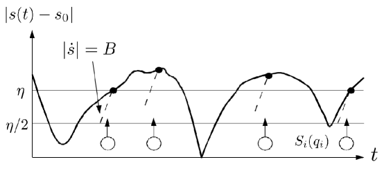
Figure 4: Visual explanation of the demonstration of Lemma 2.6. $s$ is repeatedly escaping a $\eta$-interval around $s_{0}$ ($\bullet$). Because $|\dot{s}|$ is upper bounded by $B$, then $s$ is out of the $\eta/2$-interval during non negligible time intervals (dashed lines represent $|\dot{s}|=B$). $q_{k}$ (resp. $y_{j}$) is repeatedly attracted away from $Q_{k}(s_{0})$ (resp. $Y_{j}(s_{0})$) by $Q_{k}(s)$ (resp. $Y_{j}(s)$) (arrows)

If $s$ does not converge towards $s_{0}$, it is repeatedly out of a $[s_{0}-\eta,s_{0}+\eta]$ interval, denoted $\eta$-interval:

$$\exists\eta>0,\forall t>0,\exists t^{s}>t,|s(t^{s})-s_{0}|>\eta$$

In Figure 4, $t^{s}$ time instants are represented by $\bullet$.

We can then use the upper-bounds (9) and (10) on $s$, $x_{i}$, $y_{j}$ and $z_{k}$ to show the boundedness of the $s$ dynamics

$$D(s_{in}-M^{m})-\sum_{i=1}^{N_{x}}\alpha^{m}_{i}x^{m}_{i}-\sum_{j=1}^{N_{y}}\beta^{m}_{j}(0)y^{m}_{j}-\sum_{k=1}^{N_{z}}\rho^{m}_{k}z^{m}_{k}\leq\dot{s}\leq Ds_{in}$$ (21)

so that

$$|\dot{s}|\leq B$$

with $\displaystyle B=\max\left(Ds_{in},-D(s_{in}-M^{m})+\sum_{i=1}^{N_{x}}\alpha^{m}_{i}x^{m}_{i}+\sum_{j=1}^{N_{y}}\beta^{m}_{j}(0)y^{m}_{j}+\sum_{k=1}^{N_{z}}\rho^{m}_{k}z^{m}_{k}\right)$.
Then, every time $s$ is out of the $\eta$-interval, it must also have been out of the $\eta/2$-interval during a time interval of minimal duration $A(\eta)=\frac{1}{B}\frac{\eta}{2}$. (For a visual explanation see the dashed lines of Figure 4, representing the increase caused by $|\dot{s}|=B$).

If for some $t^{s}$ we have $s(t^{s})\geq s_{0}+\eta$, we then have that $s(t^{s})\geq s_{0}+\eta/2$ during the whole time-interval $[t^{s}-A(\eta),t^{s}]$. We can thus lower bound the dynamics of $q_{k}$ (resp. $y_{j}$) during that time-interval:

$$\begin{array}[]{ll}\dot{q}_{k}&=f_{k}(Q_{k}(s))-f_{k}(q_{k})\\ &>f_{k}(Q_{k}(s_{0}+\eta/2))-f_{k}(q_{k})\\ \textrm{and}\\ \dot{y}_{j}&>(\beta_{j}(s_{0}+\eta/2,y_{j})-D)y_{j}\\ &=(\beta_{j}(s_{0}+\eta/2,y_{j})-\beta_{j}(s_{0}+\eta/2,Y_{j}(s_{0}+\eta/2)))y_{j}\end{array}$$

Now the convergence of $q_{k}$ to $Q_{k}(s_{0})$ (resp. $y_{j}$ to $Y_{j}(s_{0})$) is defined as

$$\forall\epsilon>0,\exists t^{q}>0,\forall t>t^{q},|q_{k}(t)-Q_{k}(s_{0})|<\epsilon(\textrm{resp. }|y_{j}(t)-Y_{j}(s_{0})|<\epsilon)$$ (22)

since we can pick $\epsilon$ such that $\epsilon<Q(s_{0}+\eta/4)-Q(s_{0})$ (resp. $\epsilon<\min(Y_{j}(s_{0}+\eta/4)-Y_{j}(s_{0}),Y_{j}(s_{0})-Y_{j}(s_{0}-\eta/4))$), we then have, for $t>t_{q}$, that $q_{k}(t)<Q(s_{0}+\eta/4)$ (resp. $Y_{j}(s_{0}-\eta/4)<y_{j}(t)<Y_{j}(s_{0}+\eta/4)$). Taking our $t^{s}$ larger than the corresponding $t^{q}+A(\eta)$, we then have for all time $t\,\in\,[t^{s}-A(\eta),t^{s}]$

$$\begin{array}[]{ll}\dot{q}_{k}&>f_{k}(Q_{k}(s_{0}+\eta/2))-\left(f_{k}(Q_{k}(s_{0})+\epsilon)\right)\\ &>f_{k}(Q_{k}(s_{0}+\eta/2))-f_{k}(Q_{k}(s_{0}+\eta/4))=C^{q}(\eta)>0\\ \textrm{and}\\ \dot{y}_{j}&>(\beta_{j}(s_{0}+\eta/2,Y_{j}(s_{0})+\epsilon)-\beta_{j}(s_{0}+\eta/2,Y_{j}(s_{0}+\eta/2)))y_{j}\\ &>(\beta_{j}(s_{0}+\eta/2,Y_{j}(s_{0}+\eta/4))-\beta_{j}(s_{0}+\eta/2,Y_{j}(s_{0}+\eta/2)))y_{j}\\ &>(\beta_{j}(s_{0}+\eta/2,Y_{j}(s_{0}+\eta/4))-\beta_{j}(s_{0}+\eta/2,Y_{j}(s_{0}+\eta/2)))Y_{j}(s_{0}-\eta/4)\\ &=C^{y}(\eta)>0\end{array}$$

with $C^{q}(\eta)>0$ since $f_{k}$ is an increasing function of $q_{k}$, and $C^{y}(\eta)>0$ since $\beta_{j}$ is a decreasing function of $y_{j}$

We then define

$$C(\eta)=\min\left(C^{q}(\eta),C^{y}(\eta)\right)$$

If we then choose $\epsilon$ such that $\epsilon<\frac{C(\eta)\cdot A(\eta)}{2}$, then $|q_{k}(t^{s})-q_{k}(t^{s}-A(\eta))|>2\epsilon$ (resp. $|y_{j}(t^{s})-y_{j}(t^{s}-A(\eta))|>2\epsilon$), and we see that the increase of $q_{k}$ (resp. $y_{j}$) makes it eventually get out of the $\epsilon$-interval around $Q_{k}(s_{0})$ (resp. $Y_{j}(s_{0})$). This is a contradiction, so that implication $iii=>i$ (resp. $v=>i$) holds.

Alternatively, if for some $t^{s}$ we have $s(t^{s})\leq s_{0}-\eta$, then we can upper bound the dynamics of $q_{k}$ (resp. $y_{j}$) during the $[t^{s}-A(\eta),t^{s}]$ time-interval:

$$\begin{array}[]{ll}\dot{q}_{k}&<f_{k}(Q_{k}(s_{0}-\eta/2))-f_{k}(q_{k})\\ \textrm{and}\\ \dot{y}_{j}&<(\beta_{j}(s_{0}-\eta/2,y_{j})-D)y_{j}\\ &=(\beta_{j}(s_{0}-\eta/2,y_{j})-\beta_{j}(s_{0}-\eta/2,Y_{j}(s_{0}-\eta/2)))y_{j}\end{array}$$

and the same arguments hold, with

$$\begin{array}[]{ll}\dot{q}_{k}<f_{k}(Q_{k}(s_{0}-\eta/2))-f_{k}(Q_{k}(s_{0})-\eta/4)=C(\eta)<0\\ \textrm{and}\\ \dot{y}_{j}<(\beta_{j}(s_{0}-\eta/2,Y_{j}(s_{0}-\eta/4))-\beta_{j}(s_{0}-\eta/2,Y_{j}(s_{0}-\eta/2)))Y_{j}(s_{0}+\eta/4)\\ =C(\eta)<0\end{array}$$

and finally $\epsilon<\frac{-C(\eta)\cdot A(\eta)}{2}$ which causes the contradiction. $\Box$

2.4 The equilibria correspond to the substrate subsistence concentrations

In this section we present the equilibria of the generalized competition model (7). The first equilibrium of this model corresponds to the extinction of all the microorganisms species:

$$\begin{array}[]{l}E_{0}=(s_{in}\ ,\ 0,\ldots,0\ ,\ 0,\ldots,0\ ,\ 0,\ldots,0\ ,\ Q_{1}(s_{in}),\ldots,Q_{N}(s_{in}))\end{array}$$

This equilibrium is globally attractive if the input substrate concentration $s_{in}$ is not high enough for the species’ growth to compensate their withdrawal of the chemostat by the output flow $D$, that is if $\forall i,\alpha_{i}(s_{in})\leq D$ and $\forall j,\beta_{j}(s_{in},0)\leq D$ and $\forall k,\gamma_{k}(Q_{k}(s_{in}))\leq D$ (proof of this result is easy and we omit it; for getting a clear idea of the demonstration, see [1] and [2] for the Monly and Q-only cases). We suppose that we are not in this situation through the following hypothesis:

Hypothesis 5

We assume that one of the following condition is satisfied:

• $\exists i,\alpha_{i}(s_{in})>D$

• $\exists j,\beta_{j}(s_{in},0)>D$

• $\exists k,\gamma_{k}(Q_{k}(s_{in}))>D$

This guarantees that, at least for one of the families of species, there exists some index $i$, $j$, $k$ and some associated unique $s^{x\star}_{i},s^{y\star}_{j},s^{z\star}_{k}<s_{in}$ (denoted "subsistence concentration") such that

$$\begin{array}[]{l}\alpha_{i}(s^{x\star}_{i})=D\\ \beta_{j}(s^{y\star}_{j},Y_{j}(s^{y\star}_{j}))=D\quad\textrm{with}\quad s^{y\star}_{j}+Y_{j}(s^{y\star}_{j})=s_{in}\\ \gamma_{k}(Q_{k}(s^{z\star}_{k}))=D\end{array}$$

Note that in the C-model, there exists an infinity of $s\in[S^{y}_{j}(0),s_{in})$ verifying $\beta_{j}(s,Y_{j}(s))=D$. The value $s^{y\star}_{j}$ is then the substrate concentration required for having species $j$ remaining alone in the chemostat at equilibrium. It has to satisfy $s^{y\star}_{j}+Y_{j}(s^{y\star}_{j})=s_{in}$ because of (8) that imposes $M=s+y_{j}=s_{in}$ at equilibrium.

We number these species such that

$$\begin{array}[]{l}0<s^{x\star}=s^{x\star}_{1}<s^{x\star}_{2}<\ldots<s^{x\star}_{n_{x}}\leq s_{in}\\ 0<S^{y}_{1}(0)<S^{y}_{2}(0)<\ldots<S^{y}_{n_{y}}(0)\leq s_{in}\\ 0<s^{z\star}=s^{z\star}_{1}<s^{z\star}_{2}<...<s^{z\star}_{n_{z}}\leq s_{in}\\ \textrm{with }\forall(i,j,k)\in(\{1,...,n_{x}\},\{1,...,n_{y}\},\{1,...,n_{z}\}),\,s^{x\star}_{i}\neq S^{y}_{j}(0)\neq s^{z\star}_{k}\end{array}$$ (23)

where $n_{x}$, $n_{y}$ and $n_{z}$ are the number or free bacteria, attached bacteria and phytoplankton species having a subsistence concentration smaller than $s_{in}$ for the given $D$; all other species cannot be positive at equilibrium. Hypothesis 5 implies that at least one of $n_{x}$, $n_{y}$ and $n_{z}$ is non-zero. We denote $s^{x\star}$ and $s^{z\star}$ the lowest M- and Q- substrate subsistence concentrations. We also denote $s^{y\star}$ the substrate concentration that there would be at equilibrium if there were only attached species in the chemostat (see [7]); since it needs to satisfy (8), it requires

$$s^{y\star}+\sum_{j=1}^{n_{y}}Y_{j}(s^{y\star})=s_{in}$$

Though the sum of $Y_{j}(s^{y\star})$ spans all the relevant indices, some species might have $Y_{j}(s^{y\star})=0$ because they have $s^{y\star}<S^{y}_{j}(0)<s_{in}$. If some $n_{x}$, $n_{y}$ or $n_{z}$ is zero, we set the corresponding $s^{x\star}$, $s^{y\star}$ or $s^{z\star}$ to $s_{in}$ because none of the species from their family can survive at a substrate concentration lower than $s_{in}$, which is the higher admissible concentration.

In the previous competitive exclusion studies [1, 2, 7] these quantities were of primer importance, as they directed the result of competition. Here we show that the competition outcome is strongly linked to

$$s^{\star}=\min(s^{x\star},s^{y\star},s^{z\star})$$

which is the lowest of all subsistence concentrations. Hypothesis 5 implies that $s^{\star}<s_{in}$.

We do not consider the case where two subsistence concentrations are equal, because we suppose that the biological parameters of each species are different. In his broad historical review about competitive exclusion [15] Hardin wrote: "no two things or processes in a real world are precisely equal. In a competition for substrate, no difference in growth rate or subsistence quota can be so slight as to be neglected".

Hypothesis 6

$\forall(i,j,k)\in(\{1,...,n_{x}\},\{1,...,n_{y}\},\{1,...,n_{z}\}),\,s^{x\star}_{i}\neq S^{y}_{j}(0)\neq s^{z\star}_{k}$

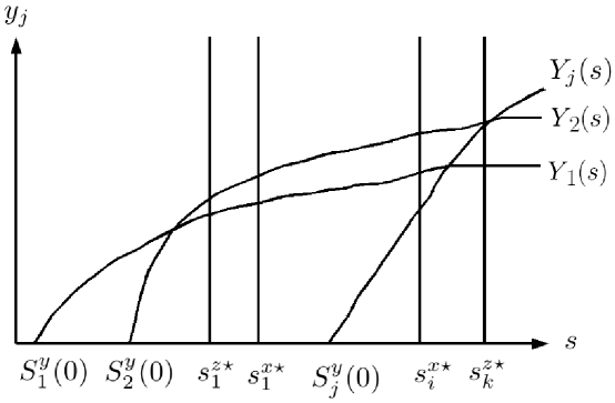
Figure 5: Subsistence concentrations of the M-model ($s^{x\star}_{i}$) and Q-model ($s^{z\star}_{k}$) species, and equilibrium biomass $Y_{j}(s)$ of the attached species, which enable these species to have a growth rate equal to the dilution rate $D$, and thus to be at equilibrium. We see that M- and Q-model species cannot coexist at equilibrium because they have only one fixed subsistence concentration, and $s$ cannot be simultaneously equal to several of these concentrations. On the contrary, attached species can coexist with others at equilibrium because they can have a growth equal to $D$ for any $s\in[S^{y}_{j}(0),s_{in})$, by adjusting their biomass concentration to $Y_{j}(s)$ (see definition (16))

The subsistence concentrations and $Y_{j}(s)$ functions are presented in Figure 5. In this figure, we see that no free species model can coexist at equilibrium because $s$ cannot simultaneously be equal to $s^{x\star}_{i}$ and $s^{z\star}_{k}$. On the contrary, attached species verifying Hypothesis 5 can support different $s$ value at equilibrium (between $S^{y}_{j}(0)$ and $s_{in}$), so that there exist equilibria where one M- or D-model species coexist with one or several attached species (see Figure 5 for a graphical explanation). On those equilibria, only the attached species verifying

$$S^{y}_{j}(0)<s^{x\star}_{i}\quad(\textrm{resp. }S^{y}_{j}(0)<s^{z\star}_{k})$$ (24)

can coexist as they can be at equilibrium at the subsistence concentration of the M-model (resp. D-model) species, by having a biomass equal to $Y_{j}(s^{x\star}_{i})$ (resp. $Y_{j}(s^{x\star}_{k})$).

For these considerations, we can enunciate the following proposition which does not need to be proved:

Lemma 2.7

For a given $s_{0}$ substrate concentration, we have

• $x_{i}$ is $s_{0}$-compliant if $s_{i}^{x*}=s_{0}$;

• $y_{j}$ is $s_{0}$-compliant is $S_{j}(0)<s_{0}$;

• $z_{k}$ is $s_{0}$-compliant if $s_{k}^{z*}=s_{0}$

It ensues that, for the corresponding C-species we have

$$Y_{j}(s_{0})>0$$

which means that they can be at positive equilibrium under dilution rate $D$ and substrate concentration $s_{0}$. Thus, the $s^{\star}$-compliant species are:

• only the $s^{\star}$-compliant C-species, if $s^{\star}=s^{y\star}$

• $x_{1}$ and all the $s^{\star}$-compliant C-species, if $s^{\star}=s^{x\star}$

• $z_{1}$ and all the $s^{\star}$-compliant C-species, if $s^{\star}=s^{z\star}$

We now present all these equilibria and their stability in M-, C- and Q-only substrate competitions.

2.5 M-only equilibria

$$\begin{array}[]{l}E^{x}_{i}=(s^{x\star}_{i}\ ,\ 0,\ldots,x_{i}^{\star},\ldots,0\ ,\ 0,\ldots,0\ ,\ 0,\ldots,0\ ,\ Q_{1}(s^{x\star}_{i}),\ldots,Q_{N_{z}}(s^{x\star}_{i}))\\ \textrm{with }\ x_{i}^{\star}=s_{in}-s^{x\star}_{i}\end{array}$$

each of these M-only equilibria corresponds to the winning of competition by free bacteria species $i$; such an equilibrium only exists for $i\,\in\,\{0,\cdots,n_{x}\}$ (all other species cannot survive at a substrate level lower than $S_{in}$ fot the given $D$). In a competition between several free bacteria, eqilibrium $E^{x}_{1}$ (with lowest substrate subsistence concentration $s^{x\star}_{1}$) is asymptotically globally stable, while all the others are unstable [1].

2.6 Q-only equilibria

$$\begin{array}[]{l}E^{z}_{k}=(s^{z\star}_{k}\ ,\ 0,\ldots,0\ ,\ 0,\ldots,0\ ,\ 0,\ldots,z_{k}^{\star},\ldots,0\ ,\ Q_{1}(s^{z\star}_{k}),\ldots,Q_{N_{z}}(s^{z\star}_{k}))\\ \textrm{with }\ z_{k}^{\star}=\frac{s_{in}-s^{z\star}_{k}}{Q_{k}(s^{z\star}_{k})}\end{array}$$

Similarly to M-only equilibria, each of these phytoplankton only equilibria correspond to the winning of competition by phytoplankton species $k$; such an equilibrium only exists for $k\,\in\,\{0,\cdots,n_{z}\}$. In a competition between several phytoplankton species, equilibrium $E^{z}_{1}$ (with lowest substrate subsistence concentration $s^{z\star}_{1}$) is asymptotically globally stable, while all the others are unstable [2].

2.7 C-only equilibria

We denominate $G$ a subset of $\{1,\cdots,n_{y}\}$ representing any C-species coexistence. For example if we want to speak about species 1, 5 and 7 coexistence, then we use $G=\{1,5,7\}$. We then define $E^{y}_{G}$ the equilibrium where these species coexist. It is composed by

• $s^{y\star}_{G}$ such that $s^{y\star}_{G}+\sum_{j\in G}Y_{j}(s^{y\star}_{G})=s_{in}$ because of (8)

• $\forall j\in G,y_{j}=Y_{j}(s^{y\star})$

• for any other $j$, $y_{j}=0$

• $\forall i\in\{1,\cdots,N_{x}\},x_{i}=0$

• $\forall k\in\{1,\cdots,N_{z}\},z_{k}=0$

• $\forall k\in\{1,\cdots,N_{z}\}),q_{k}=Q_{k}(s^{y\star}_{G})$

there exist many $E^{y}_{G}$ equilibria, corresponding to all the possible $G$ subset. The globally asymptotically stable equilibrium of a competition with only attached species is given by the choice $G=\{1,\cdots,n_{y}\}$ [7]. Note that some of the $G$ species can have a null biomass on these equilibria, as $Y_{j}(s^{y\star}_{G})$ might be null for some $j\in G$. Therefore $E_{G_{1}}^{y}$ and $E_{G_{2}}^{y}$ with $G_{1}\neq G_{2}$ are not necessarily different.

We must here introduce a technical hypothesis which will be useful later to prove hyperbolicity of the equilibria.

Hypothesis 7

For all $G$ and all $j$ : $S_{j}(0)\neq s^{y\star}_{G}$

2.8 Coexistence equilibria

As previously said in this section, there also exist equilibria where one of the free species coexist with several $s^{x\star}_{i}$- or $s^{z\star}_{k}$-compliant attached bacterial species. For a coexistence with free bacteria species we denote them $E^{(x,y)\star}_{i,G}$. They are composed of:

• $s=s^{x\star}_{i}$

• $\forall j\in G,y_{j}=Y_{j}(s^{x\star}_{i})$

• for any other $j$, $y_{j}=0$

• $\forall l\neq i,x_{l}=0$

• $\forall k\in\{1,\cdots,N_{z}\},z_{k}=0$

• $\forall k\in\{1,\cdots,N_{z}\},q_{k}=Q_{k}(s^{x\star}_{i})$

• $x_{i}=s_{in}-s^{x\star}_{i}-\sum_{j\in G}Y_{j}(s^{x\star}_{i})$ (this value will be denoted $\bar{x}_{i}^{G}$)

Similarly, for a coexistence with phytoplankton species we denote them $E^{(z,y)\star}_{k,G}$ . They are composed of:

• $s=s^{z\star}_{k}$

• $\forall j\in G,y_{j}=Y_{j}(s^{z\star}_{k})$

• for any other $j$, $y_{j}=0$

• $\forall i\in\{1,\cdots,N_{x}\},x_{i}=0$

• $\forall l\neq k,z_{l}=0$

• $\forall l\in\{1,\cdots,N_{z}\},q_{l}=Q_{l}(s^{z\star}_{k})$

• $z_{k}=\frac{s_{in}-s^{z\star}_{k}-\sum_{j\in G}Y_{j}(s^{z\star}_{k})}{Q_{k}(s^{z\star}_{k})}$ (this value will be denoted $\bar{z}_{k}^{G}$)

To our knowledge, these equilibria have never been studied until now.

Note that some of these equilibria might be reduntant with M- or Q-only equilibria, if all the C-species represented by $G$ are not $s^{x\star}_{i}$- or $s^{z\star}_{k}$-compliant. Note also that all those equilibria do not necessarily exist in the non-negative orthant. Indeed, $\bar{x}_{i}^{G}$ and $\bar{z}_{k}^{G}$ can be negative, depending on $s_{in}$ and on the substrate subsistence concentrations. These equilibria with negative components will not be studied any further since we only consider initial conditions in the positive orthant, which is invariant. In the sequel, we will denote $E$ an equilibrium of (7) which belongs to an unspecified class.

We will now show that if $s=s^{\star}$ at equilibrium, there exists a positive equilibrium containing all $s^{\star}$-compliant species.

Lemma 2.8

 

• If $s^{\star}=s^{x\star}$ then $E^{(x,y)\star}_{1,\{1,\cdots,n_{y}\}}$ is in the positive orthant.

• If $s^{\star}=s^{y\star}$ then $E^{y\star}_{\{1,\cdots,n_{y}\}}$ is in the positive orthant.

• If $s^{\star}=s^{z\star}$ then $E^{(z,y)\star}_{1,\{1,\cdots,n_{y}\}}$ is in the positive orthant.

Proof:

• If $s^{\star}=s^{x\star}$, then all $y_{j}=Y_{j}(s^{x\star})\geq 0$ at equilibrium and $s^{y\star}+\sum_{j=1}^{n_{y}}Y_{j}(s^{y\star})=s_{in}$ implies that $s^{x\star}+\sum_{j=1}^{n_{y}}Y_{j}(s^{x\star})<s_{in}$ since $s^{x\star}<s^{y\star}$ and $Y_{j}(s)$ is non-decreasing. It directly follows that $x_{1}^{\star}=s_{in}-s^{x\star}-\sum_{j}^{n_{y}}Y_{j}(s^{x\star})>0$.

• If $s^{\star}=s^{y\star}$, then all $x_{i}$ and $z_{k}$ are zero at equilibrium and all $y_{j}=Y_{j}(s^{y\star})\geq 0$

• If $s^{\star}=s^{z\star}$, then all $y_{j}=Y_{j}(s^{z\star})\geq 0$ at equilibrium and $s^{y\star}+\sum_{j=1}^{n_{y}}Y_{j}(s^{y\star})=s_{in}$ implies that $s^{z\star}+\sum_{j=1}^{n_{y}}Y_{j}(s^{z\star})<s_{in}$ since $s^{z\star}<s^{y\star}$. It directly follows that $z_{1}^{\star}=\frac{s_{in}-s^{z\star}-\sum_{j}^{n_{z}}Y_{j}(s^{z\star})}{Q_{k}(s^{z\star})}>0$.

$\Box$

We call $E^{\star}$ the equilibrium with all $s^{\star}$-compliant species remaining in the chemostat, while all the others are excluded. Depending on the species subsistence concentrations, $E^{\star}$ can be one of the previously presented equilibria:

• if $s^{\star}=s^{y\star}$ then $E^{\star}=E^{y\star}_{\{1,\cdots,n_{y}\}}$: only the $s^{\star}$-compliant C-species remain in the chemostat.

• if $s^{\star}=s^{x\star}$ then $E^{\star}=E^{(x,y)\star}_{1,\{1,\cdots,n_{y}\}}$: the best free bacteria species (lowest $s^{x\star}_{i}$) remains in the chemostat with all the $s^{x\star}_{i}$-compliant C-species.

• if $s^{\star}=s^{z\star}$ then $E^{\star}=E^{(z,y)\star}_{1,\{1,\cdots,n_{y}\}}$: the best phytoplankton species (lowest $s^{z\star}_{k}$) remains in the chemostat with all the $s^{z\star}_{k}$-compliant C-species.

In the next section, we present an important global stability result for this equilibrium.

3 Statement and demonstration of the Main Theorem: competitive exclusion or coexistence in the generalized competition model

This theorem states that all the $s^{\star}$-compliant species (those who can be at equilibrium with substrate subistence concentration $s^{\star}$, which is the lowest of all $s^{x\star}.s^{y\star},s^{z\star}$) coexist in the chemostat at equilibrium, while all the others are excluded.

Main Theorem 1

In the generalized competition model (7), if Hypotheses 1–7 hold, then all the solutions of the system, having $x_{i}(0),y_{j}(0),z_{k}(0)>0$ for all $s^{*}$-compliant species, converge asymptotically towards equilibrium $E^{\star}$.

Structure of the proof: In a first step we reduce system (7) to the mass balance surface. Then we present a non decreasing lower bound $L(t)$ for $s(t)$, and use it to demonstrate that $s$ converges towards $s^{\star}$. Finally only the $s^{*}$-compliant species have a large enough substrate concentration to remain in the chemostat, so that all other M-, Q-, and C-model species are washed out. The final step consists in showing that the convergence result that we showed on the mass-balance surface can be extended to the whole non-negative orthant.

Remark 3

It is not restrictive to consider $x_{i}(0),y_{j}(0),z_{k}(0)>0$ for the solutions of the system since species with null initial condition can be ignored, so that we can then consider a smaller dimensional system.

3.1 Step 1: we consider the system on the mass balance surface and in the region where $q_{k}\,\in\,(Q_{k}^{0},Q_{k}^{m})$ for all $k\,\in\{1,...,N_{z}\}$

Lemma 2.5 indicates that $q_{k}$ reaches $(Q_{k}^{0},Q_{k}^{m})$ in finite time, and in (8) we showed that the total concentration of intra and extracellular substrate in the chemostat $M$ converges to $s_{in}$.

We denote "$\Sigma$", the generalized competition model (7) on the mass balance surface defined by

$$M=s+\sum_{i=1}^{N_{x}}x_{i}+\sum_{j=1}^{N_{y}}y_{j}+\sum_{k=1}^{N_{z}}q_{k}z_{k}=s_{in}$$ (25)

For the remainder of the demonstration we will study system $\Sigma$, and we will later show that its asymptotic convergence towards an equilibrium has the same behaviour as the initial model (7). While studying system $\Sigma$, we will however retain all the states of the original system and the expressions of the equilibria; $\Sigma$ is then defined by the addition of the invariant constraint (25).

3.2 Step 2: we propose a non decreasing lower bound $L(t)$ for $s$

The main obstacle for the demonstration of the Main Theorem was the possibility that $s$ would repeatedly be lower than $s^{\star}$ and repeatedly be higher than $s_{n}^{\star}=\max(s^{x*}_{n_{x}},s^{z*}_{n_{z}})$, which would generate an oscillating behaviour. In order to eliminate this possibility we build a non decreasing lower bound for $s$, which converges towards $s_{1}^{\star}$. We now present such a lower bound, which will be used to show that $s$ converges to $s^{\star}$ in the next sections.

Lemma 3.1

In system $\Sigma$

$$L(t)=\min\left(\min_{k}(S^{z}_{k}(q_{k}(t))),\min_{j}(S^{y}_{j}(y_{j}(t)),s^{\star},s(t)\right)$$

is a non decreasing lower bound for $s$

Proof:

We know that the right derivative of $L$ is the derivative of one of the function which realizes the minimum. In four cases we show that this right derivative is non negative.

• Case 1: If $S^{z}_{k}(q_{k}(t))$ realizes the minimum then its derivative is non negative, because $S^{z}_{k}(q_{k})$ goes towards $s$ (see (15)).

• Case 2: If $S^{y}_{j}(y_{j}(t))$ realizes the minimum then its derivative is non negative, because $S^{y}_{j}(s)$ goes towards $s$ (see (20)).

• Case 3: If $s(t)$ realizes the minimum then we examine its dynamics $\dot{s}$ for system $\Sigma$ (i.e. on the mass balance equilibrium manifold). We replace $s_{in}$ by $s+\sum_{i}x_{i}+\sum_{j}y_{j}+\sum_{k}q_{k}z_{k}$:

  $$\dot{s}=\sum_{i}(D-\alpha_{i}(s))x_{i}+\sum_{j}(D-\beta_{j}(s,y_{j}))y_{j}+\sum_{k}\left(Dq_{k}-\rho_{k}(s)\right)z_{k}$$

  which is equivalent to, from the definition (11) of $Q_{k}(s)$ :

  $$\dot{s}=\sum_{i}(D-\alpha_{i}(s))x_{i}+\sum_{j}(D-\beta_{j}(s,y_{j}))y_{j}+\sum_{k}\left(Dq_{k}-\gamma_{k}(Q_{k}(s))Q_{k}(s)\right)z_{k}$$

  Then

  • for all $i$, $s\leq s^{\star}$ gives us $\alpha_{i}(s)\leq D$, so that the first sum is non negative;

  • for all $j$, $s\leq S^{y}_{j}(y_{j}))$ gives us $\beta_{j}(s,y_{j})\leq\beta_{j}(S^{y}_{j}(y_{j}),y_{j})=D)$, so that the second sum is non negative;

  • for all $k$, $s\leq S^{z}_{k}(q_{k})$ gives us $Q_{k}(s)\leq q_{k}$, and $s\leq s^{\star}$ gives us $\gamma_{k}(Q_{k}(s))\leq\gamma_{k}(Q_{k}(s_{k}^{z\star}))=D$ so that the third sum is also non negative.

  Finally we obtain

  $$\dot{s}\geq 0$$

• Case 4: If $s^{\star}$ realizes the minimum, we know that its right derivative is null and thus non negative.

$\Box$

3.3 Step 3: we demonstrate that $s$ converges towards $s^{\star}$

Lemma 3.2

In system $\Sigma$

$$\lim_{t\rightarrow+\infty}s(t)=s^{\star}$$

Proof:

We first show, by contradiction, that the substrate concentration $s(t)$ cannot converge towards any constant value other than $s^{\star}$. Suppose the reverse hypothesis, i.e. $\lim_{t\rightarrow+\infty}s(t)=\bar{s}\neq s^{\star}$. Through Lemma 2.6, we then have that $\lim_{t\rightarrow+\infty}q_{k}(t)=Q_{k}(\bar{s})$ and $\lim_{t\rightarrow+\infty}y_{j}(t)=Y_{j}(\bar{s})$.

If $\bar{s}<s^{\star}$,

• $\alpha_{i}(\bar{s})<D$ for all $i$ so that all $x_{i}$ go to $0$

• $\gamma_{k}(Q_{k}(\bar{s}))<D$ for all $k$ implies that all $z_{k}$ go to $0$

So that we have a contradiction with mass balance equilibrium (25), as the total substrate (in the medium + in the biomasses) at equilibrium $\bar{s}+\sum_{j=1}^{N_{y}}Y_{j}(\bar{s})$ will be lower than $s^{y\star}+\sum_{j=1}^{N_{y}}Y_{j}(s^{y\star})=s_{in}$.

If $\bar{s}>s^{\star}$ we must consider three cases:

• if $s^{\star}=s^{x\star}_{1}$ then $\alpha_{i}(\bar{s})>D$ implies that $x_{1}$ diverges to $+\infty$, which is in contradiction with the boundedness shown in (9).

• if $s^{\star}=s^{z\star}_{1}$ then $\gamma_{1}(Q_{1}(\bar{s}))>D$ implies that $z_{1}$ diverges to $+\infty$, which is in contradiction with the boundedness shown in (10).

• if $s^{\star}=s^{y\star}$ then we have a contradiction with mass balance equilibrium (25), because $\bar{s}+\sum_{j=1}^{N_{y}}Y_{j}(\bar{s})$ will be higher than $s^{y\star}+\sum_{j=1}^{N_{y}}Y_{j}(s^{y\star})\leq s_{in}$.

Hence the impossibility of convergence of $s$ towards any $\bar{s}$ other that $s^{\star}$ is proven.

We now demonstrate the lemma by contradiction. We assume that

$$s\textrm{ does not converge towards }s^{\star}$$

which, from the previous remark means that $s$ does not converge to any constant value.

Remark 4

As $s$ does not converge towards $s^{\star}$, we know that the $q_{k}$ do not converge towards $Q_{k}(s^{\star})$ (see Lemma 2.6)

We consider two cases, which both lead to a contradiction, on the basis of a reasoning which is close to the demonstration developed to prove Lemma 2.6.

$\bullet$ Case $a$: $L$ attains $s^{\star}$ in finite time
In Appendix A we show that a contradiction occurs.
Idea : $s$ cannot stay higher than $s^{\star}$ without converging to $s^{\star}$, because this would cause $x_{1}$ or $z_{1}$ to diverge, or $s+\sum_{j=1}^{N_{y}}Y_{j}(s)$ to be always higher than $s_{in}$ without converging to $s_{in}$ .

$\bullet$ Case $b$: $L$ never attains $s^{\star}$
See Appendix B.
Idea : If $s$ did not converge to $s^{\star}$, the non decrease of $L$ and its attraction by $s$ would cause it to reach $s^{\star}$.

In both cases we found a contradiction, so that the proof of Lemma 3.2 is complete.

$\Box$

3.4 Step 4: all the $s^{\star}$-compliant species remain in the chemostat, while the others are excluded

In this section we show that, as $s$ converges towards $s^{\star}$ in model $\Sigma$, all the free species with substrate subsistence concentration higher than $s^{\star}$ are washed out of the chemostat because their growth $\alpha_{i}(s)$ or $\gamma_{k}(q_{k})$ cannot stay high enough to compensate the output dilution rate $D$. Finally, all the $s^{\star}$-compliant species able to be at equilibrium with a substrate concentration $s^{\star}$ remain in the chemostat.

Lemma 3.3

In system $\Sigma$ all the solutions with positive initial conditions for the $s^{*}$-compliant species converge to $E^{\star}$.

Proof:

For all the $x_{i}$ and $z_{k}$ species such that $\alpha_{i}(s^{\star})<D$ and $\gamma_{k}(Q_{k}(s^{\star}))<D$, it is straigthforward that the convergence of $s$ to $s^{\star}$ will cause their biomass to converge to $0$. If $s^{\star}=s^{y\star}$, then this is true for all the free species.

For all the $s^{\star}$-compliant C-species, we have from Lemma 2.6 that their biomass will tend to $Y_{j}(s^{\star})$, which is positive for the $s^{\star}$-compliant species and null for all the others.

Finally, if $s^{\star}=s^{x\star}$ or $s^{\star}=s^{z\star}$, then we have through the mass balance equilibrium (25) that the free species whose subsistence concentration is $s^{\star}$ will have its biomass converge to $s_{in}-s^{\star}-\sum_{j=1}^{N^{y}_{z1}}Y_{j}(s^{\star})$: all the substrate which is not present in the medium or in the attached biomasses is used by the best M- or Q-competitor. $\Box$

3.5 Step 5: convergence of the solutions for model $\Sigma$ implies convergence for model (7)

In order to extend the convergence result to the full model and thus prove our Main Theorem, we apply a classical theorem for asymptotically autonomous system [39, 2].

Lemma 3.4

All solutions of system (7) with positive initial conditions for the $s^{*}$-compliant species converge to $E^{*}$ defined in section 2.7.

Remark 5

While, up to here, we simply had considered $\Sigma$ as the same system as (7), in the same dimension, except that it was restricted to (25), we will now equivalently explicitely include (25) into system (7) to obtain $\Sigma$ in the form of a system that has one dimension less than (7) by omitting the $s$ coordinate. Since both representations of $\Sigma$ are equivalent, the previously proven stability results are still valid in the new representation, with the exception that convergence takes place towards equilibria directly derived from these presented in sections 2.5-2.8 by omitting the $s$ coordinate. These new equilibria are differentiated from the original ones by adding a  $\tilde{}$  , so that an arbitrary equilibrium is denoted $\tilde{E}$.

Proof:

System $\Sigma$ can be written as follows :

$$\begin{array}[]{l}\left\{\begin{split}\dot{x}_{i}&=\left(\alpha_{i}\left(s_{in}-\sum_{l=1}^{N_{x}}x_{l}-\sum_{m=1}^{N_{y}}y_{m}-\sum_{r=1}^{N_{z}}q_{r}z_{r}\right)-D\right)x_{i}\\ \dot{y}_{j}&=\left(\beta_{j}\left(s_{in}-\sum_{l=1}^{N_{x}}x_{l}-\sum_{m=1}^{N_{y}}y_{m}-\sum_{r=1}^{N_{z}}q_{r}z_{r},y_{j}\right)-D\right)y_{j}\\ \dot{z}_{k}&=(\gamma_{k}(q_{k})-D)z_{k}\\ \dot{q}_{k}&=\rho_{k}\left(s_{in}-\sum_{l=1}^{N_{x}}x_{l}-\sum_{m=1}^{N_{y}}y_{m}-\sum_{r=1}^{N_{z}}q_{r}z_{r}\right)-f_{k}(q_{k})\end{split}\right.\\ \textrm{ for }i\in\{1,\cdots,N_{x}\},j\in\{1,\cdots,N_{y}\},k\in\{1,\cdots,N_{z}\}\\ \end{array}$$ (26)

where the $s$ state has been removed compared to (7). In order to recover model (7), we should add the equation

$$\dot{M}=D(s_{in}-M)$$

which we interconnect with (26) by replacing every $s_{in}$ in (26) with $M$. It is this interconnection that we will now study.

In the first part of the proof, we will show that every solution of (7) converges to an equilibrium $E$. We will then show by induction that all the solutions that do not converge to $E^{*}$ have an initial condition with some $x_{i}=0$, $y_{j}=0$ or $z_{k}=0$ for some $s^{*}$-compliant species. Thus, all the solutions with $x_{i}\neq 0,y_{j}\neq 0,z_{k}\neq 0$ for the $s^{*}$-compliant species converge to $E^{*}$.

For that, we will use Theorem F.1 from [2]. We will therefore first compute the stable manifolds of all equilibria of $\Sigma$:

• The stable manifold of $\tilde{E}^{*}$ is of dimension $N_{x}+N_{y}+2N_{z}$. It is constituted of all the initial conditions which verify $x_{i}(0),y_{j}(0),z_{k}(0)>0$ for $s^{*}$-compliant species and $x_{i}(0),y_{j}(0),z_{k}(0)\geq 0$ for all other species, as well as $q_{k}\geq 0$ for all $k$ (see Lemma 3.3).

• The stable manifold of $\tilde{E}_{0}$ is of dimension $N_{x}-n_{x}+N_{y}-n_{y}+2N_{z}-n_{z}$. It is constitued of all the initial conditions which verify $x_{1}(0)=\ldots=x_{n_{x}}(0)=0$, $y_{1}(0)=\ldots=y_{n_{y}}(0)=0$ and $z_{1}(0)=\ldots=z_{n_{z}}(0)=0$. The only species that can be present at the initial condition are those that cannot survive for the given $D$ and $s_{in}$. Indeed, if any $x_{i}(0)>0$ for $i\leq n_{x}$ (or similar $y_{j}(0)>0$ or $z_{k}(0)>0$), one can apply Lemma 3.3. to the reduced order system containing these species to show that convergence does not take place towards $\tilde{E}_{0}$. Conversely, any initial condition with $x_{1}(0)=\ldots=x_{n_{x}}(0)=0$, $y_{1}(0)=\ldots=y_{n_{y}}(0)=0$ and $z_{1}(0)=\ldots=z_{n_{x}}(0)=0$ generates a solution that goes to $\tilde{E}_{0}$ since for the other species we have:

  • $\dot{x}_{i}<(\alpha_{i}(s_{in})-D)x_{i}$, with $\alpha_{i}(s_{in})-D<0$ for all $i>n_{x}$ because of the definition of $n_{x}$ presented in (23);

  • $\dot{y}_{j}<(\beta_{j}(s_{in},y_{j})-D)y_{j}$, with $\beta_{j}(s_{in},0)-D<0$ for all $j>n_{y}$, because of the definition of $n_{y}$;

  • $\dot{z}_{k}<(\gamma_{k}(Q_{k}(s_{in}))-D)z_{k}$, with $\gamma_{k}(Q_{k}(s_{in}))-D)<0$ for all $k>n_{z}$ because of the definition of $n_{z}$.

• The dimension of the stable manifold of any other $\tilde{E}$ can be computed from Lemma 3.3. To an equilibrium $\tilde{E}$ corresponds a substrate value $\tilde{s}$ ($>s^{*}$ by definition of $s^{*}$). Lemma 3.3 indicates that solutions of $\Sigma$ converge towards an equilibrium corresponding to $\tilde{s}$, if there is no smaller subsistance concentration corresponding to a species present in the system (for free species) and if all M-, Q- and C-species that are $\tilde{s}$-compliant are present in the corresponding equilibrium. The stable manifold of $\tilde{E}$ must therefore be constrained to initial conditions that verify $x_{i}(0)=0$, $y_{j}(0)=0$ and $z_{k}(0)=0$ for all species that are $s$-compliant for some $s\leq\tilde{s}$ and that are not positive in $\tilde{E}$. Having set all these values to zero, it is indeed clear that $\tilde{s}$ is the $s^{\star}$ as defined in Lemma 3.3 of the reduced order system (without the aforementionned $x_{i},y_{j}$ and $z_{k}$ coordinates). All solutions defined in Lemma 3.3 of this system then converge to $\tilde{E}$, which justifies our definition of the stable manifold of $\tilde{E}$. Its dimension is $N_{x}+N_{y}+2N_{z}-n_{\tilde{E},\tilde{s}}$, where $n_{\tilde{E},\tilde{s}}$ is the number of $s$-compliant species (for some $s\leq\tilde{s}$) that are not present in $\tilde{E}$.

Through Lemma 3.3, we have in fact shown that all solutions of $\Sigma$ in the non-negative orthant converge to an equilibrium. Indeed, for a given initial condition, either it belongs to the stable manifold of $\tilde{E}_{0}$ or, eliminating from the system all species that are null at the initial time necessarily sets it in a form where Lemma 3.3 can be applied (which shows convergence to an equilibrium).

The dimension of the stable manifold of any equilibrium $E$ will therefore be the one of $\tilde{E}$ plus $1$. The hypotheses of Theorem F.1 from [2] are indeed all verified:

• The whole system (7) is bounded (see section 2.1)

• The equilibria of system $\Sigma$ are hyperbolic (see Appendix C.2-C.6).

• There are no cycles of equilibria in system $\Sigma$. Indeed, if we analyze the potential transition between two equilibria, both equilibria must belong to the same face, so that convergence takes place to the one corresponding to the smallest value of $s$. A potential sequence of equilibria would then be characterized by a decreasing value of $s$ at each equilibrium, which prevents it from cycling.

We can then conclude from this theorem that all solutions of (7) tend to an equilibrium. We are then left with checking to what equilibrium they tend.

Before continuing this proof, we need to detail $n_{\tilde{E},\tilde{s}}$. In the case of $\tilde{E}=\tilde{E}^{*}$ and $\tilde{s}=s^{*}$, we have $n_{\tilde{E},\tilde{s}}=0$ (by definition, all $s^{*}$-compliant species are present in $E^{*}$ and there is no other species that is compliant for smaller values of $s$). Otherwise, we necessarily have $n_{\tilde{E},\tilde{s}}>0$. Indeed, we know that $\tilde{s}>s^{*}$, so that all species present in $E^{*}$ are compliant for some $s<\tilde{s}$; as such, in order to have $n_{\tilde{E},\tilde{s}}=0$, $\tilde{E}$ would need to at least contain all species that are present in $\tilde{E}^{*}$. In such a case no $S$ and $Q$ species can be present in $\tilde{E}^{*}$ (otherwise, it could not be present in $\tilde{E}$ also for a different value of $s$). Defining $J$ the set of C-species that are present in $E^{*}$ and writing (25) for $E^{*}$ then yields

$$M=s^{*}+\sum_{j\,\in\,J}Y_{j}(s^{*})=s_{in}$$

Equality (25) should also be valid in $\tilde{s}>s^{*}$ so that

$$s_{in}=\tilde{s}+\sum_{i=1}^{N_{x}}x_{i}+\sum_{j=1}^{N_{y}}y_{j}+\sum_{k=1}^{N_{z}}q_{k}z_{k}>\tilde{s}+\sum_{j\,\in\,J}Y_{j}(\tilde{s})>s_{in}$$

where we have the last inequality (which leads to a contradiction) because $Y_{j}(s)$ is an increasing function. We can then conclude that, for all $\tilde{E}\neq\tilde{E}^{*}$, $n_{\tilde{E},\tilde{s}}>0$, and at least one $s^{\star}$-compliant species species must be null.

In order to check to what equilibrium solutions of (7) tend, we use an induction argument, by supposing that our Main Theorem has been proven up to $N-1$ species, which we use for the proof for $N$ species. Along with the fact that the stability result is trivial for $1$ species (classical Monod model, [2], classical Droop model, [24] and generalized Contois model, [7]), this will conclude our proof.

Let us consider a system of $N$ species with equilibrium $E^{*}$ as defined earlier. This equilibrium contains positive species (which are $s^{\star}$-compliant) and null species (which are not $s^{\star}$-compliant).

Imposing, for one of the not $s^{\star}$-compliant species, $x_{i}=0$ (or $y_{j}=0$ or $z_{k}=0$) for the initial condition, sets us in the framework where we have $N-1$ species present in the system. Also, since this species did not belong to the positive ones in $E^{\star}$, its absence does not change anything into which equilibrium is the one corresponding to the smallest subsistance concentration, which remains $E^{\star}$. We can then apply the induction hypothesis, which indicates that all such initial conditions initiate solutions that converge to $E^{\star}$ (as long as the $s^{\star}$-compliant species have positive initial condition).

Studying now the equilibrium $E_{0}$, we know from the beginning of the proof that its stable manifold is of dimension $N_{x}-n_{x}+N_{y}-n_{y}+2N_{z}-n_{z}+1$. As was done for $\Sigma$, it is directly apparent that any initial condition with $x_{1}(0)=\ldots=x_{n_{x}}(0)=0$, $y_{1}(0)=\ldots=y_{n_{y}}(0)=0$ and $z_{1}(0)=\ldots=z_{n_{x}}(0)=0$ generates a solution that has all species exponentially go to zero. Finally, the analysis of the $\dot{s}$ equation shows that it has the form $\dot{s}=D(s_{in}-s)-F(t)$ with $F(t)$ exponentially going to zero so that $s$ goes to $s_{in}$ and all such solutions go to $E_{0}$.

We can now consider all the other equilibria. Let an equilibrium $E$ corresponding to a substrate concentration $\tilde{s}$ ($>s^{*}$ by definition). As we have seen in our analysis of $\Sigma$, the stable manifold of the corresponding $\tilde{E}$ is of dimension $N_{x}+N_{y}+2N_{z}-n_{\tilde{E},\tilde{s}}$, so that the stable manifold of $E$ is of dimension $N_{x}+N_{y}+2N_{z}-n_{\tilde{E},\tilde{s}}+1$. Let us set ourselfes in the situation where all $n_{\tilde{E},\tilde{s}}$ species are set to zero at the initial time and all others are positive. We can then consider the system with only the remaining $N_{x}+N_{y}+2N_{z}-n_{\tilde{E},\tilde{s}}$ positive species and the substrate. We have seen that, in this case, all solutions of the corresponding reduced order $\Sigma$ go to $\tilde{E}$ which means that $\tilde{s}$ is the “$s^{*}$” defined in Lemma 3.4 for the reduced order system. Since the reduced order system contains less than $N$ species because $n_{\tilde{E},\tilde{s}}>0$, we conclude that all solutions of the full system (7) that have zero initial condition for all $n_{\tilde{E},\tilde{s}}$ species and positive values for all $N_{x}+N_{y}+2N_{z}-n_{\tilde{E},\tilde{s}}$ others converge to $\tilde{E}$. We have then exhibited an invariant manifold of dimension $N_{x}+N_{y}+2N_{z}-n_{\tilde{E},\tilde{s}}+1$ for which all solutions go to $E$; this corresponds to the predicted dimension of the stable manifoldof $E$. No solution with some of the $n_{\tilde{E},\tilde{s}}$ species positive (among which there is at least on $s^{*}$-compliant species) at the initial time can then converge to $E$.

This completes the proof of our Main Theorem since all solutions go to an equilibrium and we have exhibited the stable manifold of all equilibria other than $E^{*}$. These manifolds cannot go into the region where $x_{i},y_{j}$ or $z_{k}>0$ for all $s*-compliant$ species because at least one of them is in the corresponding $n_{\tilde{E},\tilde{s}}$-set. All initial conditions in the region where $x_{i},y_{j}$ or $z_{k}>0$ for all $s*-compliant$ species therefore generate solutions that go to $E^{*}$. $\Box$

4 Discussion

4.1 How $D$ and $s_{in}$ both determine competition outcome

In M- and Q-only competitions, the outcome of competition is mainly determined by $D$, which fixes the $s^{x\star}_{i}$ and $s^{z\star}_{k}$ M- and Q-substrate subsistence concentrations; the role of $s_{in}$ is to allow the best competitor (already determined by the value of $D$) to settle the reactor, or to cause it to be washed out with all the others. On the contrary in C-only competition, both controls have important roles: $D$ fixes the $Y_{j}(s)$ functions, while $s_{in}$ determines the equilibrium, where $s^{y\star}+\sum_{j}Y_{j}(s^{y\star})=s_{in}$. With a low enough $s_{in}$, only few C-species will settle the chemostat ($s^{y\star}$ being low in this case, there will be few $s^{y\star}$-compliant species, with non-null $Y_{j}(s^{y\star})$), whereas a high enough $s_{in}$ can enable all C-species to coexist.

Finally, in a mixed competition the dilution rate $D$ fixes all the M- and Q-substrate subsistence concentrations $s^{x\star}_{i}$ and $s_{k}^{z\star}$, as well as the $Y_{j}(s)$ functions, while the input substrate concentration $s_{in}$ selects the species remaining in the reactor, by limiting the available nutrients, and thus the biomasses present in the reactor at equilibrium. Figure 6 gives an example between three competitors.

Figure 6: Mixed 3 class competition outcome depends both on the dilution rate $D$ and input substrate concentration $s_{in}$. The solid lines represent the influence of $D$, which fixes the subsistence concentrations of one M-model ($s^{x\star}$) and Q-model ($s^{z\star}$) species, and the equilibrium biomass $Y(s)$ of one C-species. As the free bacteria species has a too high subsistence concentration $s^{x\star}>s^{z\star}$ it will be outcompeted and excluded. The three numerated zones represent the influence of $s_{in}$. Zone 1 ($s_{in}\leq S^{y}(0)$) : no species remain at equilibrium. Zone 2 ($S^{y}(0)<s_{in}\leq s^{z\star}+Y(s^{z\star})$) : only the C-species remains at equilibrium. Zone 3 ($s_{in}>s^{z\star}+Y(s^{z\star})$) : the attached bacteria and phytoplankton species coexist.

On this figure the $s^{x\star}$ and $s^{z\star}$ values and the $Y(s)$ function are fixed by $D$. Here $s^{z\star}_{1}$ is lower than $s^{x\star}_{1}$, so that the free bacteria species will be outcompeted and washed out. Then the value of $s_{in}$ determines wether

1. no species remain at equilibrium

2. only the attached bacterial species remains at equilibrium, as there is not enough input substrate to feed both attached bacteria and phytoplankton species: because $s^{y\star}+Y(s^{y\star})=s_{in}$ and $s_{in}<s^{z\star}+Y(s^{z\star})$, we know that $s^{y\star}<s^{z\star}$, so that $s^{\star}=s^{y\star}$, and only the C-species remains in the reactor.

3. both the attached bacteria and phytoplankton species remain in the chemostat: here $s_{in}>s^{z\star}+Y(s^{z\star})$ and $s_{in}=s^{y\star}+Y(s^{y\star})$ give $s^{y\star}>s^{z\star}$, so that $s^{\star}=s^{z\star}$ and the phytoplankton species remains in the reactor, coexisting with the $s^{z\star}$-compliant C-species.

In this last case $D$ has fixed the $s^{z\star}$ substrate equilibrium value and the $Y(s)$ function, and at equilibrium the total substrate in the chemostat, equal to $s_{in}$, will be composed of

• the substrate in the medium $s^{z\star}$ (which is fixed by $D$ and does not depend on $s_{in}$);

• the attached bacterial species internal substrate $Y(s^{z\star})$ (which is also fixed by $D$ only);

• the phytoplankton species internal substrate $Q(s^{z\star}))z^{\star}=s_{in}-Y(s^{z\star})-s^{z\star}$, which depends on $s_{in}$.

By going from left to right in Figure 6, starting with $s_{in}=0$, it is possible to imagine the input substrate concentration increase, thus enabeling more and more substrate $s=s_{in}$ at equilibrium (zone 1). Then in zone 2 the C-species is present at equilibrium, and as $s_{in}$ increases, more and more biomass $Y(s)$ is present at equilibrium. Finally $Y(s^{z\star})$ is the maximal biomass for which the attached species needs less substrate at equilibrium than the phytoplankton species to have a growth rate equal to $D$. After that it has to coexist with the phytoplankton species: when $s_{in}$ increases higher than $s^{z\star}+Y(s^{z\star})$ it enables more and more Q-biomass $z^{\star}$, while keeping substrate concentration $s=s^{z\star}$ and C-biomass $y=Y(s^{z\star})$.

4.2 Originiality of the demonstration

The demonstration explains how the state variables evolve, and its originality for the study of uniquely phytoplankton (or bacteria) species can be summed up in three points.
First, we chose to study the substrate evolution instead of ignoring it after the classical mass balance equilibrium transformation $s=s_{in}-\sum_{i}x_{i}-\sum_{j}y_{j}-\sum_{k}{q_{k}z_{k}}$.
Then, the definition of the $S^{y}_{j}$ and $S^{z}_{k}$ functions enabled to gather most information on the substrate axis: instead of having separate information on $1+N_{x}+N_{y}+2N_{z}$ axes we obtained a one dimensional view on these dynamics (Figure 2 and 3), where all the $S^{y}_{j}(y_{j})$ and $S^{z}_{k}(q_{k})$ go towards $s$. We have thus turned a complex $1+N_{x}+N_{y}+2N_{z}$ dimensional problem into a simpler one: "how do $s$ and the $S^{y}_{j}(y_{j})$ and $S^{z}_{k}(q_{k})$ behave on the substrate axis, and what are the consequences for the biomasses?".
Finally the definition of the non decreasing lower bound $L(t)$ (section 3.2) and its convergence towards $s^{\star}$ (section 3.3) were the last steps for this demonstration to emerge.

Free species pure competitions (with one class of species among Monod or Droop) for substrate lead to the "survival of the fittest", the fittest being the species with lowest substrate requirement $s^{\star}$. On the contrary, Contois-only competition lead to a coexistence equilibrium, because biomass dependence gives attached bacterial species the capability to remain at equilibrium for different substrate concentrations in the range $[S^{y}_{j}(0),s_{in})$ (see Figure 5). Monod and Droop species are mutually exclusive, which leads to the pessimization principle of adaptative dynamics [40] : "mutation and natural selection lead to a deterioration of the environmental condition, a Verlenderung. We end up with the worst of all possible environment." On the contrary attached species are coexistence-compliant thanks to biomass dependence, which nuances the pessimization principle: "some species could live in worse environments ($s=\min_{j}(S^{y}_{j}(0))$ being the worse one) but if there is enough substrate for other species, they can coexist." (see Figure 6 and discussion)

5 Conclusion

In this paper a demonstration was given for the outcome of competition between phytoplankton and bacteria. Three scenarios are possible, depending both on the dilution rate $D$ and input substrate concentration $s_{in}$ (see discussion for precisions):

• only the best free competitor remains in the chemostat;

• only some attached bacterial species coexist at equilibrium;

• a new equilibrium (never studied before) is attained, where the best free competitor coexists with all the $s^{\star}$-compliant attached bacterial species.

Since the introduction of the concept of evolution, with its link to competitive exclusion [15] and the "paradox of phytoplankton" [11] modelling has tried to apprehend competition, and to predict or control it. Our contribution in this framework was to extend the results proven in the N-species Monod model, N-species Droop model and N-species Contois model, where the outcome of competition was predicted and explained with mathematical arguments, accompanied by ecological interpretations.

An important conclusion in this type of competition is that attached bacteria are likely to be present in a pure culture of microalgae. This may have very important consequences on the ecological point of view, since such natural coexistence between a phytoplanktonic species and attached bacteria may have lead to co-evolution, where the best association between phytoplankton and bacteria have been progressively selected.

Appendix A Step 3 - Case $a$: $L$ attains $s^{\star}$ in finite time

In this case

• if $s^{\star}=s^{z\star}_{1}$ we consider Figure 7 where $L$ attains $s^{\star}$ after a finite time $t^{L}$:

  $$\forall t\geq t^{L},L(t)=s_{1}^{\star}$$

  

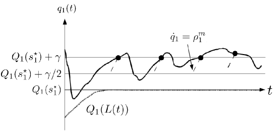
  Figure 7: Visual explanation of the demonstration of Lemma 3.2 - Case 1: $L$ attains $s^{\star}$ in finite time $t^{L}$ (Q-model). $i)$ $q_{1}$ is repeatedly higher than $Q_{1}(s^{\star})+\theta$ ($\bullet$). $ii)$ Because $\dot{q}_{1}$ is upper bounded by $\rho^{m}_{1}$, so that $q_{1}$ is higher than $Q_{1}(s^{\star})+\theta/2$ during non negligible time intervals (dashed lines represent $\dot{q}_{1}=\rho^{m}_{1}$). Thus $z_{1}$ diverges, which is a contradiction.

  Substep 3a.1: after a finite time larger than $t^{L}$, $q_{1}$ is repeatedly higher than $Q_{1}(s^{\star})+\theta$.

  Since $\min_{i}(S^{z}_{k}(q_{k}))\geq L$, we know that

  $$\forall t>t^{L},q_{1}(t)\geq Q_{1}(s^{\star})$$

  As $s$ does not converge to $s^{\star}$, we also know from Lemma 2.6 that $q_{1}$ does not converge towards $Q_{1}(s^{\star})$:

  $$\exists\theta>0,\forall t>0,\exists t^{q}>t,|q_{1}(t^{q})-Q_{1}(s^{\star})|>\theta$$

  Those two facts imply that the repeated exits of $q_{1}(t)$ from the $\theta$-interval around $Q_{1}(s^{\star})$ take place above $Q_{1}(s^{\star})$ for any $t^{q}>t^{L}$, so that, in that case, we have $q_{1}(t^{q})>Q_{1}(s^{\star})+\theta$. In Figure 7, such $t^{q}$ time instants are represented by $\bullet$.

  Substep 3a.2: $q_{1}$ is higher than $Q_{1}(s^{\star})+\theta/2$ during non negligible time intervals.

  Since the $q_{1}$-dynamics are upper bounded with

  $$\dot{q}_{1}\leq\rho^{m}_{1}$$

  we know that every time $q_{1}$ is higher than $Q_{1}(s^{\star})+\theta$, it has been higher than $Q_{1}(s^{\star})+\theta/2$ during a time interval of minimal duration $A(\theta)=\frac{\theta}{2\rho^{m}_{1}}$. On Figure 7, $\dot{q}_{1}=\rho^{m}_{1}$ is represented by the dashed lines.

  Substep 3a.3: then $z_{1}$ diverges, which is impossible

  From time $t^{L}$ on, we have that $q_{1}\geq Q_{1}(s^{\star})\Rightarrow\gamma_{1}(q_{1})\geq D$, so that $z_{1}(t)$ is non decreasing. During each of the time interval where $q_{1}$ is higher than $Q_{1}(s^{\star})+\theta/2$, the increase of $z_{1}$ is lower bounded by

  $$\dot{z}_{1}=\gamma_{1}(Q_{1}(s^{\star})+\theta/2)-D=C(\theta)>0$$

  so that every $t^{q}$ time we have

  $$z_{1}(t^{q})-z_{1}(t^{q}-A(\theta))>C(\theta)A(\theta)$$

  As such increases occurs repeatedly, and as $z_{1}$ is non decreasing, $z_{1}$ diverges. This is a contradiction because $z_{1}$ is upper bounded (see (10)).
  

• if $s^{\star}=s^{x\star}_{1}$ then the non convergence of $s$ to $s^{\star}$, and the fact that $s\geq s^{\star}$ will cause $s$ to be non negligibly "away" from $s^{\star}$, so that $x_{1}$ will diverge, causing a contradiction with (9). This is exactly the same demonstration as above (in the case $s^{\star}=s^{z\star}_{1}$) without needing the $q_{k}$ study.

• if $s^{\star}=s^{y\star}$ then $s+\sum_{j=1}^{N_{y}}Y_{j}(s)$ will always be higher than $s_{in}=s^{y\star}+\sum_{j=1}^{N_{y}}Y_{j}(s^{y\star})$ without converging to $s_{in}$, which is in contradiction with (25).

Appendix B Step 3 - Case $b$: $L$ never attains $s^{\star}$

In this case $L(t)$ converges towards a value $\hat{L}\in(0,s^{\star}]$, because it is non decreasing and bounded in $[0,s^{\star}]$, so that

$$\forall\epsilon>0,\exists t^{L}(\epsilon)>0,\forall t>t^{L}(\epsilon),\arrowvert L(t)-\hat{L}\arrowvert<\epsilon$$

We consider the neighborhood of $\hat{L}$ in Figure 8.

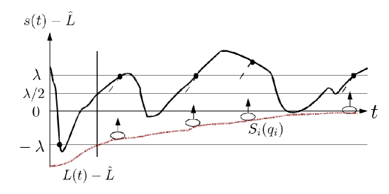
Figure 8: Visual explanation of the demonstration of Lemma 3.2 - Case 2: $L$ never attains $s^{\star}$. $i)$ $s$ is repeatedly higher than $\hat{L}+\lambda$ ($\bullet$). $ii)$ $\dot{s}$ is upper bounded by $Ds_{in}$, so that $s$ is higher than $\hat{L}+\lambda/2$ during non negligible time intervals (dashed lines represent $\dot{s}=Ds_{in}$) $iii)$ during such a time intervals $L=\min_{k}(S^{z}_{k}(q_{k}))$ (or $\min_{j}(S^{y}_{j}(y_{j}))$) is increasing non negligibly towards $s$, so that $L$ cannot both converge towards $\hat{L}$ and stay lower than $\hat{L}$ during the whole time interval: there is a contradiction.

Substep 3b.1: after a finite time, $s$ is repeatedly higher than $\hat{L}+\lambda$.

Since, from the beginning of the proof of Lemma 3.2, we know that $s$ does not converge to any constant value, hence not to $\hat{L}$,

$$\exists\lambda>0,\forall t>0,\exists t^{s}>t,|s(t^{s})-\hat{L}|>\lambda$$

Since $L$ is increasing and converges to $\hat{L}$, it reaches $\hat{L}-\lambda$ in finite time $t^{L}(\lambda)$. After this finite time, $s$ is higher than $\hat{L}+\lambda$ on every $t^{s}$ time instants, which are represented by $\bullet$ in Figure 8.

Substep 3b.2: $s$ is higher than $\hat{L}+\lambda/2$ during non negligible time intervals.

Because of the boundedness of $\dot{s}$

$$\dot{s}\leq Ds_{in}$$

every time $s$ is higher than $\hat{L}+\lambda$, it has been higher than $\hat{L}+\lambda/2$ during a non negligible time interval of minimal duration $A(\lambda)=\frac{\lambda}{2Ds_{in}}$. On Figure 8 the case $\dot{s}=Ds_{in}$ is represented by dashed lines.

Substep 3b.3: $L=\min_{k}(S^{z}_{k}(q_{k}))$ (or $\min_{j}(S^{y}_{j}(y_{j}))$) is increasing non negligibly towards $s$, so that $L$ cannot both converge towards $\hat{L}$ and stay lower than $\hat{L}$ during the whole time interval: there is a contradiction.

Like in previous proofs, we are interested in what happens during the $[t^{s}-A(\lambda),t^{s}]$ time-interval, with $t^{s}-A(\lambda)>t^{L}(\epsilon)$ (for some $\epsilon<\lambda$). Since, during this time-interval, $s(t)>\hat{L}+\lambda/2$ and $L<\hat{L}$, we know that there exists a $k$ such that $L(t^{s})=S^{z}_{k}(q_{k}(t^{s}))<\hat{L}$, or a $j$ such that $L(t^{s})=S^{y}_{j}(y_{j}(t^{s}))<\hat{L}$.

For both this step (3b.3) we choose to first only present arguments for the case $L(t^{s})=\min_{k}(S^{z}_{k}(q_{k}))$; almost similar arguments for the case $L(t^{s})=\min_{j}(S^{y}_{j}(y_{j}))$ will then be briefly presented.

• if $L(t^{s})=\min_{k}(S^{z}_{k}(q_{k}))$, then during the whole considered time-interval, as $S^{z}_{k}(q_{k})$ was increasing, we know that

  $$\hat{L}-\epsilon<L\leq S^{z}_{k}(q_{k})\leq S^{z}_{k}(q_{k}(t^{s}))<\hat{L}$$ (27)

  so that $Q_{k}(\hat{L}-\epsilon)<q_{k}(t)<Q_{k}(\hat{L})$. For the $k$ species, the dynamics of $q_{k}$ can then be lower bounded:

  $$\dot{q}_{k}\geq\rho_{k}(\hat{L}+\lambda/2)-f_{k}(Q_{k}(\hat{L}))$$

  and then

  $$\dot{q}_{k}\geq\rho_{k}(\hat{L}+\lambda/2)-\rho_{k}(\hat{L})=G_{k}(\lambda)$$

  positive, so that the increase of $q_{k}$ during the $[t^{s}-A(\lambda),t^{s}]$ time-interval is also lower bounded:

  $$q_{k}(t^{s})-q_{k}(t^{s}-A(\lambda))\geq G_{k}(\lambda)A(\lambda)=H_{k}(\lambda)$$

  Since $Q_{k}=S^{z^{-1}}_{k}$ is locally Lipschitz with constant $K$ (because $f^{\prime}_{k}>0$), we have

  $$\begin{array}[]{ll}q_{k}(t^{s})-q_{k}(t^{s}-A(\lambda))&=Q_{k}(S^{z}_{k}(q_{k}(t^{s})))-Q_{k}(S^{z}_{k}(q_{k}(t^{s}-A(\lambda))))\\ &<K\left[S^{z}_{k}(q_{k}(t^{s}))-S^{z}_{k}(q_{k}(t^{s}-A(\lambda)))\right]\end{array}$$

  so that the corresponding increase of $S^{z}_{k}(q_{k})$ is lower bounded with

  $$\begin{array}[]{ll}S^{z}_{k}(q_{k}(t^{s}))-S^{z}_{k}(q_{k}(t^{s}-A(\lambda)))&\geq\frac{1}{K}H_{k}(\lambda)\end{array}$$

  and then

  $$S^{z}_{k}(q_{k}(t^{s}-A(\lambda)))<\hat{L}-\frac{1}{K}H_{k}(\lambda)$$

  which implies the same higher bound for $L$:

  $$L(t^{s}-A(\lambda))<\hat{L}-\frac{1}{K}H_{k}(\lambda)$$

  By choosing $\epsilon<\frac{1}{K}H_{k}(\lambda)$, this inequality is contradictory with (27) so that Case 2 is not possible

• if $L(t^{s})=\min_{j}(S^{y}_{j}(y_{j}))$, then the same arguments can be developped for the $j$ species, with a lower bound $G_{j}(\lambda)$ on the $y_{j}$ dynamics:

  $$G_{j}(\lambda)=\beta_{j}(\hat{L}+\lambda/2,Y_{j}(\hat{L}))-\beta_{j}(\hat{L},Y_{j}(\hat{L}))>0$$

  and then an increase of variable $y_{j}$ at least equal to $H_{j}(\lambda)=G_{j}(\lambda)A(\lambda)$ followed by a non negligible increase of $L$

  $$L(t^{s}-A(\lambda))<\hat{L}-\frac{1}{K}H_{j}(\lambda)$$

  because $Y_{j}$ is locally Lipschitz. Finally a contradiction also occurs when $\epsilon<\frac{1}{K}H_{j}(\lambda)$:

  $$L(t^{s}-A(\lambda))<\hat{L}-\epsilon$$

Appendix C Computation of system $\Sigma$ Jacobian Matrix and eigenvalues for all the equilibria

Computation of the Jacobian Matrix of system $\Sigma$, with $s=s_{in}-\sum_{i=1}^{N_{x}}x_{i}-\sum_{j=1}^{N_{y}}y_{j}-\sum_{k=1}^{N_{z}}q_{k}z_{k}$.

$$\left(\begin{array}[]{cccc}J^{xx}&J^{xy}&J^{xz}&J^{xq}\\ J^{yx}&J^{yy}&J^{yz}&J^{yq}\\ J^{zx}&J^{zy}&J^{zz}&J^{zq}\\ J^{qx}&J^{qy}&J^{qz}&J^{qq}\end{array}\right)$$

where

$$\begin{array}[]{l}J^{xx}_{ii}=\alpha_{i}(s)-D-\frac{\partial\alpha_{i}}{\partial s}x_{i}\quad\textrm{and}\quad\forall l\neq i,J^{xx}_{il}=-\frac{\partial\alpha_{i}}{\partial s}x_{i}\\ J^{xy}_{ij}=-\frac{\partial\alpha_{i}}{\partial s}x_{i}\\ J^{xz}_{ik}=-\frac{\partial\alpha_{i}}{\partial s}x_{i}q_{k}\\ J^{xq}_{ik}=-\frac{\partial\alpha_{i}}{\partial s}x_{i}z_{k}\\ \textrm{and}\\ J^{yx}_{ji}=-\frac{\partial\beta_{j}}{\partial s}y_{j}\\ J^{yy}_{jj}=\beta_{j}(s,y_{j})-D+\frac{\partial\beta_{j}}{\partial y_{j}}y_{j}-\frac{\partial\beta_{j}}{\partial s}y_{j}\quad\textrm{and}\quad\forall l\neq j,J^{yy}_{jl}=-\frac{\partial\beta_{j}}{\partial s}y_{j}\\ J^{yz}_{jk}=-\frac{\partial\beta_{j}}{\partial s}y_{j}q_{k}\\ J^{yq}_{jk}=-\frac{\partial\beta_{j}}{\partial s}y_{j}z_{k}\\ \textrm{and}\\ J^{zx}_{ki}=0\\ J^{zy}_{kj}=0\\ J^{zz}_{kk}=\gamma_{k}(q_{k})-D\quad\textrm{and}\quad\forall l\neq k,J^{zz}_{kl}=0\\ J^{zq}_{kk}=\frac{\partial\gamma_{k}}{\partial q_{k}}z_{k}\quad\textrm{and}\quad\forall l\neq k,J^{zq}_{kl}=0\\ \textrm{and}\\ J^{qx}_{ki}=-\frac{\partial\rho_{k}}{\partial s}\\ J^{qy}_{kj}=-\frac{\partial\rho_{k}}{\partial s}\\ J^{qz}_{kl}=-\frac{\partial\rho_{k}}{\partial s}q_{l}\\ J^{qq}_{kk}=-\frac{\partial\rho_{k}}{\partial s}z_{k}-\frac{\partial f_{k}}{\partial q_{k}}\quad\textrm{and}\quad\forall l\neq k,J^{qq}_{kl}=-\frac{\partial\rho_{k}}{\partial s}z_{l}\\ \end{array}$$

Fortunately for eigenvalue computations, at equilibria the null biomasses will simplify the matrix:

• when $x_{i}=0$, then the whole $i^{th}$ line gives eigenvalue $\alpha_{i}(s)-D$ (denoted "$x_{i}$-eigenvalue") and can be deleted, as well as the $i^{th}column$;

• when $y_{j}=0$ then the whole $N_{x}+j^{th}$ line gives eigenvalue $\beta_{j}(s,y_{j})-D$ (denoted "$y_{j}$-eigenvalue") and can be deleted, as well as the $N_{x}+j^{th}$ corresponding column;

• when $z_{k}=0$ then the whole $N_{x}+N_{y}+k^{th}$ line gives eigenvalue $\gamma_{k}(q_{k})-D$ (denoted "$z_{k}$-eigenvalue") and can be deleted, as well as the $N_{x}+N_{y}+k^{th}$ column; in a second step, the whole $N_{x}+N_{y}+N_{z}+k^{th}$ column can also be deleted and gives eigenvalue $\frac{-\partial f_{k}}{\partial q_{k}}$ (denoted "$q_{k}$-eigenvalue"), as well as the $N_{x}+N_{y}+N_{z}+k^{th}$ line.

C.1 Complete washout equilibrium

With this in hand, we see that for equilibrium $\tilde{E}_{0}$ ($x_{i}=y_{j}=z_{k}=0$) the Jacobian matrix is triangular, so that the eigenvalues lay on the diagonal. They are:

• $\alpha_{i}(s_{in})-D$

• $\beta_{j}(s_{in},0)-D$

• $\gamma_{k}(Q_{k}(s_{in}))-D$

• $-\frac{\partial f_{k}}{\partial q_{k}}\quad\textrm{(negatives)}$

We denote $n_{x}$, $n_{y}$, $n_{z}$ the number of M-, C- and Q- species verifying the inequalities of Hypothesis 5, and thus having the possibility to be at equilibrium with a positive biomass, under controls $D$ and $s_{in}$. Each of these species has a positive corresponding eigenvalue on this equilibrium, so that equilibirum $\tilde{E}_{0}$ has $n_{x}+n_{y}+n_{z}$ positive eigenvalues, and $N_{x}-n_{x}+N_{y}-n_{y}+2N_{z}-n_{z}$ negative eigenvalues.

C.2 M-only equilibria

For equilibrium $E^{x}_{i}$ we get all the previously cited x-,y-, z-and q-eigenvalues:

• $\alpha_{l}(s^{x\star}_{i})-D$ whose signs are the same as $sign(s^{x\star}_{i}-s^{x\star}_{l})$

• $\beta_{j}(s^{x\star}_{i},0)-D$ which are positive if the $j^{th}$ species is $s^{x\star}_{i}$-compliant, or negative else;

• $\gamma_{k}(Q_{k}(s^{x\star}_{i}))-D$ whose signs are the same as $sign(s^{x\star}_{i}-s^{z\star}_{k})$

• $\frac{-\partial f_{k}}{\partial q_{k}}$ which are all negative

and the remaining eigenvalue corresponds to the positive $x_{i}$-only dynamics:

$$\dot{x}_{i}=(\alpha_{i}(s_{in}-x_{i})-D)x_{i}$$

which yields the eigenvalue $-\frac{\partial\alpha_{i}}{\partial s}x_{i}^{\star}$ for free bacteria species $i$. Each free species with a substrate subsistence concentration $s^{x\star}_{l}$ or $s^{z\star}_{k}$ lower than $s^{x\star}_{i}$ gives a positive eigenvalue. Among all the $E^{x}_{i}$ equilibria, only $E^{x}_{1}$ is stable if and only if $s^{\star}=s_{1}^{x\star}<s_{1}^{z\star}$, and if all the C-species are not $s^{x\star}_{1}$-compliant.

C.3 Q-only equilibria

For Equilibrium $E^{z}_{k}$ we get all the

• $x$-eigenvalues whose signs are the sign of $sign(s^{z\star}_{k}-s^{x\star}_{i})$;

• $y$-eigenvalues: as previously, $y$-eigenvalues are positive if the corresponding C-species is $s^{z\star}_{k}$-compliant and negative else;

• $z_{l}$-eigenvalues whose signs are the sign of $sign(s^{z\star}_{k}-s^{z\star}_{l})$;

• $q_{l}$-eigenvalues for all $l\neq k$ (negative);

and the remaining eigenvalues correspond to the positive $(z_{k},q_{k})$-only dynamics:

$$\left\{\begin{array}[]{lll}\dot{z}_{k}&=&(\gamma_{k}(q_{k})-D)z_{k}\\ \dot{q}_{k}&=&\rho_{k}(s_{in}-q_{k}z_{k})-f_{k}(q_{k})\end{array}\right.$$

and we obtain the following resulting matrix:

$$\left(\begin{array}[]{cccc}0&\frac{\partial\gamma_{k}}{\partial q_{k}}z_{k}\\ -\frac{\partial\rho_{k}}{\partial s}q_{k}&-\frac{\partial\rho_{k}}{\partial s}z_{k}-\frac{\partial f_{k}}{\partial q_{k}}\end{array}\right)$$

which has negative trace and positive determinant, so that its two eigenvalues are real negative. Just like before, each free species with a substrate subsistence concentration $s^{x\star}_{i}$ or $s^{z\star}_{l}$ lower than $s^{z\star}_{k}$ gives a positive eigenvalue. Among all the $E^{z}_{k}$ equilibria, only $E^{z}_{1}$ is stable if and only if $s^{\star}=s_{1}^{z\star}<s_{1}^{x\star}$, and if all the C-species are not $s^{z\star}_{1}$-compliant.

C.4 C-only equilibria

Now let us consider the $E^{y}_{G}$ equilibria for which all $j\in G$ (where $G$ represents a subset of $\{1,\ldots,N_{y}\}$) C-species coexist in the chemostat under substrate concentration $s^{y\star}_{G}$, while all the free species are washed out. $s^{y\star}_{G}$ is defined by $s^{y\star}_{G}+\sum_{j\in G}Y_{j}(s^{y\star}_{G})=s_{in}$. Note that some of the $G$ species can have a null biomass on these equilibria, as $Y_{j}(s^{y\star}_{G})$ might be null for some $j\in G$.

This gives all the

• $x$-eigenvalues whose sign are the same as the signs of $s^{x\star}_{i}-s^{y\star}_{G}$;

• $z$-eigenvalues whose sign are the same as the signs of $s^{z\star}_{k}-s^{y\star}_{G}$;

• $q$-eigenvalues (negative).

All the $y_{j}$ species who are not included in $G$ give negative eigenvalues if they are not $s^{y\star}_{G}$-compliant, and positive eigenvalues else; their eigenvalues cannot be null because of technical hypothesis 7. All the $y_{j}$ species who are included in $G$ but have a null biomass $Y_{j}(s^{y\star}_{G})$ on the $E^{y}_{G}$ equilibrium give negative eigenvalues. Now let us study the remaining matrix $J^{yy}_{G}$ which is composed of all the $j\in G$ lines of $J^{yy}$, for which $Y_{j}(s^{y\star}_{G})>0$, and thus $\beta_{j}(s^{y\star}_{G},Y_{j}(s^{y\star}_{G}))=D$:

$$\dot{y}_{j}=\left(\beta_{j}(s-\sum_{l}y_{l},y_{j})-D\right)y_{j}$$

which yields the Jacobian matrix:

$$J^{yy}_{G}=\left(\begin{array}[]{ccccc}-a_{1}-b_{1}&\ldots&-a_{1}&\ldots&-a_{1}\\ \vdots&\ddots&\vdots&&\vdots\\ -a_{j}&\ldots&-a_{j}-b_{j}&\ldots&-a_{j}\\ \vdots&&\vdots&\ddots&\vdots\\ -a_{n}&\ldots&-a_{n}&\ldots&-a_{n}-b_{n}\\ \end{array}\right)$$

with $a_{j}=\frac{\partial\beta_{j}}{\partial s}Y_{j}(s^{y\star}_{G})>0$ and $b_{j}=-\frac{\partial\beta_{j}}{\partial y_{j}}Y_{j}(s^{y\star}_{G})>0$.

Let us show that this matrix has only real negative eigenvalues, by using the definition of an eigenvalue $\lambda=(A+Bi)$, where $A\in\mathbb{R}$ is the real part and $B\in\mathbb{R}$ the imaginary part:

$$J^{yy}_{G}\cdot\left(\begin{array}[]{l}y_{1}\\ \vdots\\ y_{n}\end{array}\right)=(A+Bi)\left(\begin{array}[]{l}y_{1}\\ \vdots\\ y_{n}\end{array}\right)$$ (28)

We obtain $n$ equations:

$$-b_{j}y_{j}-a_{j}\sum_{l}y_{l}=(A+Bi)y_{j}$$

and thus

$$(A+Bi+b_{j})y_{j}=-a_{j}\sum_{l}y_{l}$$ (29)

If we have $A+Bi+b_{j}=0$ for some $j$, then $B=0$ and $A=-b_{j}<0$ so that we have a negative eigenvalue.
Else, isolating $y_{j}$ yields

$$y_{j}=\frac{-a_{j}\sum_{l}y_{l}}{b_{j}+A+Bi}$$

Summing over $j$, we obtain

$$\sum_{j}y_{j}=\sum_{j}\left(\frac{-a_{j}\sum_{l}y_{l}}{b_{j}+A+Bi}\right)$$

Now if $\sum_{j}y_{j}=0$, since some $y_{j}$ must be different of $0$, (29) yields, for that $j$, that $A+Bi+b_{j}=0$ so that again $B=0$ and $A=-b_{j}<0$.
Else, simplifying the sums of $y_{l}$ and $y_{j}$, this yields

$$\begin{array}[]{lll}1&=&\sum_{j}\left(\frac{-a_{j}}{b_{j}+A+Bi}\right)\\ &=&\sum_{j}\left(\frac{-a_{j}(b_{j}+A-Bi)}{(b_{j}+A)^{2}+B^{2}}\right)\\ &=&\sum_{j}\left(\frac{-a_{j}(b_{j}+A)}{(b_{j}+A)^{2}+B^{2}}\right)+i\sum_{j}\left(\frac{a_{j}B)}{(b_{j}+A)^{2}+B^{2}}\right)\end{array}$$

Since the left-hand-side is real, the imaginary part of the right-hand side must be zero, which imposes $B=0$. For thr right-hand-side to be positive, at least one of the $b_{j}+A$ must be negative, which translates into $\min_{j}(b_{j}+A)<0$ and

$$A<-\min_{j}b_{j}<0$$

We conclude from this that all eigenvalues of this matrix are real negative.

Finally, an $E^{y}_{G}$ equilibrium is stable if and only if all the C-species not contained in $G$ are not $s^{y\star}_{G}$-compliant (this is equivalent to saying that $s^{y\star}_{G}=s^{y\star},\textrm{ with }s^{y\star}=s^{y\star}_{\{1,\ldots,N_{y}\}}$), and if $s^{\star}=s^{y\star}$.

C.5 M-coexistive equilibria

In this section we consider equilibria $E^{(x,y)}_{i,G}$ where free bacteria species $x_{i}$ coexists with the C-species in $G$, a subset of $\{1,\ldots,N_{y}\}$, under substrate concentration $s^{x\star}_{i}$.

We obtain here all the

• $x_{l}$-eigenvalues ($l\neq i$) whose signs are the signs of $s^{x\star}_{i}-s^{x\star}_{l}$;

• $z$-eigenvalues whose sign is the sign of $s^{x\star}_{i}-s^{z\star}_{k}$;

• $q$-eigenvalues (negative);

$y_{j}$-eigenvalues with $j$ not in $G$ are positive if $y_{j}$ is $s^{x\star}_{i}$-compliant and negative else; $y_{j}$-eigenvalues with $j$ in $G$ but have a null biomass $Y_{j}(s^{x\star}_{i})$ give negative eigenvalues. For the remaining C-species, and species $x_{i}$, we obtain the following system:

$$\left\{\begin{array}[]{lll}\dot{x}_{i}&=&\left(\alpha_{i}(s_{in}-x_{i}-\sum_{l}y_{l})-D\right)x_{i}\\ \dot{y}_{j}&=&\left(\beta_{j}(s_{in}-x_{i}-\sum_{l}y_{l},y_{j})-D\right)y_{j}\\ \end{array}\right.$$

and the Jacobian matrix:

$$\left(\begin{array}[]{cccccc}-a_{0}&-a_{0}&\ldots&-a_{0}&\ldots&-a_{0}\\ -a_{1}&-a_{1}-b_{1}&\ldots&-a_{1}&\ldots&-a_{1}\\ \vdots&\vdots&\ddots&\vdots&&\vdots\\ -a_{j}&-a_{j}&\ldots&-a_{j}-b_{j}&\ldots&-a_{j}\\ \vdots&\vdots&&\vdots&\ddots&\vdots\\ -a_{n}&-a_{n}&\ldots&-a_{n}&\ldots&-a_{n}-b_{n}\\ \end{array}\right)$$

with $a_{0}=\frac{\partial\alpha_{i}}{\partial s}x_{i}^{\star}>0$, $a_{j}=\frac{\partial\beta_{j}}{\partial s}Y_{j}(s^{x\star}_{i})>0$ and $b_{j}=-\frac{\partial\beta_{j}}{\partial y_{j}}Y_{j}(s^{x\star}_{i})>0$ (for $j\,\in\,\{1,\cdots,n\}$). This matrix has exactly the same form has the one considered on Appendix C.4. The only difference being that the there is no “$b_{0}$” in the first element of the matrix. Defining a $b_{0}=0$, we can then conclude that all eigenvalues are real and negative because, following the development of Appendix C.4, we obtain

$$A<-\min_{j}b_{j}=0$$

Finally, only equilibrium $E^{(x,y)}_{1,\{1,\ldots,N_{y}\}}$ can be stable if and only if $s^{\star}=s^{x\star}_{1}$.

C.6 Q-coexistive equilibria

In this section we consider equilibria $E^{(z,y)}_{k,G}$ where phytoplankton species $z_{k}$ coexists with the attached species in $G$, a subset of $\{1,\ldots,N_{y}\}$, under substrate concentration $s^{z\star}_{k}$.

We obtain here all the

• $x$-eigenvalues whose signs are the signs of $s^{z\star}_{k}-s^{x\star}_{i}$;

• $z_{l}$-eigenvalues ($l\neq j$) whose sign are the signs of $s^{z\star}_{k}-s^{z\star}_{l}$;

• $q$-eigenvalues (negative);

$y_{j}$-eigenvalues with $j$ not in $G$ are positive if $y_{j}$ is $s^{z\star}_{k}$-compliant and negative else; $y_{j}$-eigenvalues with $j$ in $G$ but have a null biomass $Y_{j}(s^{z\star}_{k})$ give negative eigenvalues. For the remaining C-species, and species $z_{k}$, we obtain the following model

$$\left\{\begin{array}[]{lll}\dot{y}_{j}&=&(\beta_{j}(s_{in}-\sum_{l}y_{l}-q_{k}z_{k},y_{j})-D)y_{j}\\ \dot{z}_{k}&=&(\gamma_{k}(q_{k})-D)z_{k}\\ \dot{q}_{k}&=&\rho_{k}(s_{in}-\sum_{l}y_{l}-q_{k}z_{k})-f_{k}(q_{k})\end{array}\right.$$

and, swapping the last two equations and using $f_{k}(q_{k})=\gamma_{k}(q_{k})q_{k}$, we get the Jacobian matrix:

$$\left(\begin{array}[]{ccccccc}-a_{1}-b_{1}&\ldots&-a_{1}&\ldots&-a_{1}&-a_{1}z_{k}&-a_{1}q_{k}\\ \vdots&\ddots&\vdots&&\vdots&\vdots&\vdots\\ -a_{j}&\ldots&-a_{j}-b_{j}&\ldots&-a_{j}&-a_{j}z_{k}&-a_{j}q_{k}\\ \vdots&&\vdots&\ddots&\vdots&\vdots\\ -a_{n}&\ldots&-a_{n}&\ldots&-a_{n}-b_{n}&-a_{n}z_{k}&-a_{n}q_{k}\\ -a_{n+1}&\ldots&-a_{n+1}&\ldots&-a_{n+1}&-a_{n+1}z_{k}-b_{n+1}q_{k}-\gamma&-a_{n+1}q_{k}\\ 0&\ldots&0&\ldots&0&b_{n+1}z_{k}&0\end{array}\right)$$

with $a_{j}=\frac{\partial\beta_{j}}{\partial s}Y_{j}(s^{z\star}_{k})>0$ and $b_{j}=-\frac{\partial\beta_{j}}{\partial y_{j}}Y_{j}(s^{z\star}_{k})>0$ for $j\,\in\,\{1,\cdots,n\}$, with $a_{n+1}=\frac{\partial\rho_{k}}{\partial s}$ and $b_{n+1}=\frac{\partial\gamma_{k}}{\partial q_{k}}$. By using the definition of eigenvalue $\lambda=(A+Bi)$ (see (28)) we follow a similar path to that of Appendix C.4, we show that the eigenvalues are real and negative.

Finally, only equilibrium $E^{(z,y)}_{1,\{1,\ldots,N_{y}\}}$ can be stable if and only if $s^{\star}=s^{z\star}_{1}$.

Remark 6

The same work can be done for the whole system (7), where the eigenvalues are the same, plus the $-D$ eigenvalue which arises from mass balance dynamics (8).

Received September 2006; revised February 2007.

References

- [1] R. Armstrong and R. McGehee, “Competitive exclusion,” American Naturalist, vol. 115, p. 151, 1980.
- [2] H. Smith and P. Waltman, The theory of the chemostat. Dynamics of microbial competition. Cambridge Studies in Mathematical Biology. Cambridge University Press, 1995.
- [3] S.-B. Hsu and T.-H. Hsu, “Competitive exclusion of microbial species for a single nutrient with internal storage,” SIAM J. Appl. Math., vol. 68, pp. 1600–1617, 2008.
- [4] D. Tilman and R. Sterner, “Invasions of equilibria: tests of resource competition using two species of algae,” Oecologia, vol. 61, no. 2, pp. 197–200, 1984.
- [5] S. Hansen and S. Hubell, “Single-nutrient microbial competition: qualitative agreement between experimental and theoretically forecast outcomes,” Science, vol. 207, no. 4438, pp. 1491–1493, 1980.
- [6] D. Tilman, “Resource competition between plankton algae: An experimental and theoretical approach.,” Ecology, vol. 58, no. 22, pp. 338–348, 1977.
- [7] F. Grognard, F. Mazenc, and A. Rapaport, “Polytopic lyapunov functions for persistence analysis of competing species,” Discrete and Continuous Dynamical Systems-Series B, vol. 8, no. 1, pp. 73–93, 2007.
- [8] O. Pulz and W. Gross, “Valuable products from biotechnology of microalgae,” Applied Microbiology and Biotechnology, vol. 65, pp. 635–648, 2004. 10.1007/s00253-004-1647-x.
- [9] P. Spolaore, C. Joannis-Cassan, E. Duran, and A. Isambert, “Commercial applications of microalgae,” Journal of Bioscience and Bioengineering, vol. 101, pp. 87–96, Feb. 2006.
- [10] Y. Chisti, “Biodisel from microalgae,” Biotechnology Advances, vol. 25, pp. 294–306, 2007.
- [11] G. E. Hutchinson, “The paradox of the plankton,” The American Naturalist, vol. 95, p. 137, 1961.
- [12] M. Droop, “Vitamin and marine ecology,” J. Mar. Biol Assoc. U.K., vol. 48, pp. 689–733, 1968.
- [13] A. Sciandra and P. Ramani, “The steady states of continuous cultures with low rates of medium renewal per cell,” J. Exp. Mar. Biol. Ecol., vol. 178, pp. 1–15, 1994.
- [14] I. Vatcheva, H. deJong, O. Bernard, and N. Mars, “Experiment selection for the discrimination of semi-quantitative models of dynamical systems,” Artif. Intel., vol. 170, pp. 472–506, 2006.
- [15] G. Hardin, “The competitive exclusion principle,” Science, vol. 131, no. 3409, pp. 1292–1297, 1960.
- [16] C. Elton, Animal Ecology. Sidgwick & Jackson, LTD. London, 1927.
- [17] C. Darwin, On the Origin of Species by Means of Natural Selection, or the Preservation of Favoured Races in the Struggle for Life. John Murray, 1859.
- [18] M. Scriven, “Explanation and prediction in evolutionnary theory,” Science, vol. 130, no. 3374, pp. 477–482, 1959.
- [19] C. Jessup, S. Forde, and B. Bohannan, “Microbial experimental systems in ecology,” Advances in Ecological Research, vol. 37, pp. 273–306, 2005.
- [20] G. Gause, The Struggle for Existence. Williams and Wilkins, Baltimore, 1934.
- [21] J. Monod, “Reserches sur la croissance des cultures bacteriennes,” Paris: Herrmann et Cie, 1942.
- [22] J. Caperon and J. Meyer, “Nitrogen-limited growth of marine phytoplankton. i. changes in population characteristics with steady-state growth rate,” Deep-Sea Res., vol. 19, pp. 601–618, 1972.
- [23] K. Lange and F. J. Oyarzun, “The attractiveness of the Droop equations,” Mathematical Biosciences, vol. 111, pp. 261–278, 1992.
- [24] F. J. Oyarzun and K. Lange, “The attractiveness of the Droop equations. II: Generic uptake and growth functions,” Mathematical Biosciences, vol. 121, pp. 127–139, 1994.
- [25] O. Bernard and J.-L. Gouzé, “Transient behavior of biological loop models, with application to the Droop model,” Mathematical Biosciences, vol. 127, no. 1, pp. 19–43, 1995.
- [26] D. Contois, “Kinetics of bacterial growth: relationship between population density and species growth rate of continuous cultures,” J Gen Microbiol., pp. 40–50, 1959.
- [27] J. Leon and D. Tumpson, “Competition between two species of two complementary or substitutable resources,” J. Theor. Biol., vol. 50, pp. 185–201, 1975.
- [28] S. Hsu, K. Cheng, and S. Hubbel, “Exploitative competition of micro-organisms for two complementary nutrients in continuous culture,” SIAM J. Appl. Math., vol. 41, pp. 422–444, 1981.
- [29] H. Freedman, J. So, and P. Waltman, “Coexistence in a model of competition in the chemostat incorporating discrete delays,” SIAM J. Appl. Math., vol. 49, pp. 859–870, 1989.
- [30] P. de Leenheer and H. Smith, “Feedback control for the chemostat,” J. Math. Biol., vol. 46, pp. 48–70, 2003.
- [31] P. de Leenheer, D. Angeli, and A. Sontag, “A feedback perspective for chemostat models with crowding effects,” in Positive Systems, vol. 294 of Lecture Notes in Control and Inform. Sci, pp. 167–174, Springer-Verlag, 2003.
- [32] J. Arino, S. Pilyugin, and G. Wolkowicz, “Considerations on yield, nutrient uptake, cellular growth, and competition in chemostat models,” Canadian Applied Math Quarterly, vol. 11, pp. 107–142, (2003) [2005].
- [33] J. B. Wilson, “Mechanisms of species coexistence: twelve explanations for the hutchinson’s ’paradox of the phytoplankton’: evidence from new zealand plant communities,” New Zealand journal of Ecology, vol. 137, pp. 17–42, 1990.
- [34] A. Fredrickson and G. Stephanopoulos, “Microbial competition,” Science, vol. 213, pp. 972–979, 1981.
- [35] J. Gouzé and G. Robledo, “Feedback control for nonmonotone competition models in the chemostat,” Nonlinear Analysis: Real World Applications, pp. 671–690, 2005.
- [36] P. de Leenheer, B. Li, and H. Smith, “Competition in the chemostat : some remarks,” Canadian applied mathematics quarterly, vol. 11, no. 2, pp. 229–247, 2003.
- [37] N. Rao and E. Roxin, “Controled growth of competing species,” Journal on Applied Mathematics, vol. 50, no. 3, pp. 853–864, 1990.
- [38] P. Masci, O. Bernard, and F. Grognard, “Continuous selection of the fastest growing species in the chemostat,” in Proceedings of the IFAC conference, Seoul, Korea, 2008.
- [39] H. R. Thieme, “Convergence results and a Poicaré-Bendixson trichotomy for asymptotically autonomous differential equations,” Journal of Mathematical Biology, vol. 30, pp. 755–763, Aug. 1992.
- [40] O. Diekmann, “A beginner’s guide to adaptive dynamics,” Banach Center Publ., vol. 63, pp. 47–86, 2003.