1 Introduction

In decision-theoretic statistical settings, one receives samples $\{z_{1},\ldots,z_{n}\}\subseteq\mathcal{Z}$ drawn i.i.d. from some unknown distribution $P$ over a sample space $\mathcal{Z}$, and given a loss function $\ell$, seeks a function $f$ to minimize the risk

$$R(f):=\mathbb{E}[\ell(z,f)].$$ (1)

Since $R(f)$ is unknown, the typical approach is to compute estimates based on the empirical risk, $\widehat{R}_{{n}}(f):=\frac{1}{n}\sum_{i=1}^{n}\ell(z_{i},f)$, over a function class $\mathcal{F}$. Through this, one seeks a function $f_{n}$ with a risk close to the Bayes risk, the minimal risk over all measurable functions, which is $R_{0}:=\inf_{f}R(f)$. There is a natural tradeoff based on the class $\mathcal{F}$ one chooses, since

$$R(f_{n})-R_{0}=\left(R(f_{n})-\inf_{f\in\mathcal{F}}R(f)\right)+\left(\inf_{f\in\mathcal{F}}R(f)-R_{0}\right),$$

which decomposes the excess risk of $f_{n}$ into estimation error (left) and approximation error (right).

A common approach to addressing this tradeoff is to express $\mathcal{F}$ as a union of classes

$$\mathcal{F}=\bigcup_{j\geq 1}\mathcal{F}_{j}.$$ (2)

The model selection problem is to choose a class $\mathcal{F}_{i}$ and a function $f\in\mathcal{F}_{i}$ that give the best tradeoff between estimation error and approximation error. A standard approach to the model selection problem is the now classical idea of complexity regularization, which arose out of early works by Mallows [21] and Akaike [1]. The complexity regularization approach balances two competing objectives: the minimum empirical risk of a model class $\mathcal{F}_{i}$ (approximation error) and a complexity penalty (to control estimation error) for the class. Different choices of the complexity penalty give rise to different model selection criteria and algorithms (for example, see the lecture notes by Massart [23] and the references therein). The complexity regularization approach uses penalties $\gamma_{i}:\mathbb{N}\rightarrow\mathbb{R}_{+}$ associated with each class $\mathcal{F}_{i}$ to perform model selection, where $\gamma_{i}(n)$ is a complexity penalty for class $i$ when $n$ samples are available; usually the functions $\gamma_{i}$ decrease to zero in $n$ and increase in the index $i$. The actual algorithm is as follows: for each $i$, choose

$$\hat{f}_{i}\in\mathop{\rm argmin}_{f\in\mathcal{F}_{i}}\widehat{R}_{{n}}(f)~{}~{}~{}\mbox{and~{}select}~{}~{}~{}\widetilde{f}_{n}=\mathop{\rm argmin}_{i=1,2,\ldots}\left\{\widehat{R}_{{n}}(\hat{f}_{i})+\gamma_{i}(n)\right\}$$ (3)

as the output of the model selection procedure, where $\widehat{R}_{{n}}$ denotes the $n$-sample empirical risk. Results of several authors [11, 20, 23] show that with appropriate penalties $\gamma_{i}$ and given a dataset of size $n$, the output $\widetilde{f}_{n}$ of the procedure roughly satisfies

$$\mathbb{E}R(\widetilde{f}_{n})-R_{0}\leq\min_{i}\left[\inf_{f\in\mathcal{F}_{i}}R(f)-R_{0}+\gamma_{i}(n)\right]+\mathcal{O}\left(\frac{1}{\sqrt{n}}\right).$$ (4)

Several approaches to complexity regularization are possible, and an incomplete bibliography includes the papers [28, 16, 25, 5, 11, 20].

Oracle inequalities of the form (4) show that, for a given sample size, complexity regularization procedures trade off the approximation and estimation errors, often optimally [23]. A drawback of the above approaches is that in order to provide guarantees on the result of the model selection procedure, one needs to be able to optimize over each model in the hierarchy (that is, compute the estimates $\hat{f}_{i}$ for each $i$). This is reasonable when the sample size $n$ is the key limitation, and it is computationally feasible when $n$ is small and the samples $z$ are low-dimensional. However, the cost of fitting a large number of model classes on a large, high-dimensional dataset can be prohibitive; such data is common in modern statistical settings. In such cases, it is the computational resources—rather than the sample size—that form the key inferential bottleneck. In this paper, we consider model selection from this computational perspective, viewing the amount of computation, rather than the sample size, as the quantity whose effects on estimation we must understand. Specifically, we study model selection methods that work within a given computational budget.

An interesting and difficult aspect of the problem that we must address is the interaction between model class complexity and computation time. It is natural to assume that for a fixed sample size, it is more expensive to estimate a model from a complex class than a simple class. Put inversely, given a computational bound, a simple model class can fit a model to a much larger sample size than a rich model class. So any strategy for model selection under a computational constraint should trade off two criteria: (i) the relative training cost of different model classes, which allows simpler classes to receive far more data (thus making them resilient to overfitting), and (ii) lower approximation error in the more complex model classes.

In addressing these computational and statistical issues, this paper makes two main contributions. First, we propose a novel computational perspective on the model selection problem, which we believe should be a natural consideration in statistical learning problems. Secondly, within this framework, we provide algorithms for model selection in many different scenarios, and provide oracle inequalities on their estimates under different assumptions. Our first two results address the case where we have a model hierarchy that is ordered by inclusion, that is, $\mathcal{F}_{1}\subseteq\mathcal{F}_{2}\subseteq\mathcal{F}_{3}\subseteq\ldots$. The first result provides an inequality that is competitive with an oracle knowing the optimal class, incurring at most an additional logarithmic penalty in the computational budget. The second result extends our approach to obtaining faster rates for model selection under conditions that guarantee sharper concentration results for empirical risk minimization procedures; oracle inequalities under these conditions, but without computational constraints, have been obtained, for example, by Bartlett [8] and Koltchinskii [18]. Both of our results refine existing complexity-regularized risk minimization techniques by a careful consideration of the structure of the problem. Our third result applies to model classes that do not necessarily share any common structure. Here we present a novel algorithm—exploiting techniques for multi-armed bandit problems—that uses confidence bounds based on concentration inequalities to select a good model under a given computational budget. We also prove a minimax optimal oracle inequality on the performance of the selected model. All of our algorithms are computationally simple and efficient.

The remainder of this paper is organized as follows. We begin in Section 2 by formalizing our setting for a nested hierarchy of models, providing an estimator and oracle inequalities for the model selection problem. In Section 3, we refine our estimator and its analysis to obtain fast rates for model selection under some additional reasonable (standard) conditions. We study the setting of unstructured model collections in Section 4. Detailed technical arguments and various auxilliary results needed to establish our main theorems and corollaries can be found in the appendices.

2 Model selection over nested hierarchies

In many practical scenarios, the family of models with which one works has some structure. One of the most common model selection settings has the model classes $\mathcal{F}_{i}$ ordered by inclusion with increasing complexity (e.g. [11]). In this section, we study such model selection problems; we begin by formally stating our assumptions and giving a few natural examples, proceeding thereafter to oracle inequalities for a computationally efficient model selection procedure.

2.1 Assumptions

Our first main assumption is a natural inclusion assumption, which is perhaps the most common assumption in prior work on model selection (e.g. [11, 20]):

Assumption A.

The function classes $\mathcal{F}_{i}$ are ordered by inclusion:

$$\mathcal{F}_{1}\subseteq\mathcal{F}_{2}\subseteq\mathcal{F}_{3}\subseteq\ldots$$ (5)

We provide two examples of such problems in the next section. In addition to the inclusion assumption, we make a few assumptions on the computational aspects of the problem. Most algorithms used in the framework of complexity regularization rely on the computation of estimators of the form

$$\widehat{f}_{i}=\mathop{\rm argmin}_{f\in\mathcal{F}_{i}}\widehat{R}_{{n}}(f),$$ (6)

either exactly or approximately, for each class $i$. Since the model classes are ordered by inclusion, it is natural to assume that the computational cost of computing an empirical risk minimizer from $\mathcal{F}_{i}$ is higher than that for a class $\mathcal{F}_{j}$ when $i>j$. Said differently, given a fixed computational budget $T$, it may be impossible to use as many samples to compute an estimator from $\mathcal{F}_{i}$ as it is to compute an estimator from $\mathcal{F}_{j}$ (again, when $i>j$). We formalize this in the next assumption, which is stated in terms of an (arbitrary) algorithm $\mathcal{A}$ that selects functions $f\in\mathcal{F}_{i}$ for each index $i$ based on a set of $n_{i}$ samples.

Assumption B.

Given a computational budget $T$, there is a sequence $\{n_{i}(T)\}_{i}\subset\mathbb{N}$ such that

1. $n_{i}(T)>n_{j}(T)$ for $i<j$.

2. The complexity penalties $\gamma_{i}$ satisfy $\gamma_{i}(n_{i}(T))<\gamma_{j}(n_{j}(T))$ for $i<j$.

3. For each class $\mathcal{F}_{i}$, the computational cost of using the algorithm $\mathcal{A}$ with $n_{i}(T)$ samples is $T$. That is, estimation within class $\mathcal{F}_{i}$ using $n_{i}(T)$ samples has the same computational complexity for each $i$.

4. For all $i$, the output $\mathcal{A}\left({i},{T}\right)$ of the algorithm $\mathcal{A}$, given a computational budget $T$, satisfies

   $$\widehat{R}_{{n_{i}(T)}}(\mathcal{A}\left({i},{T}\right))-\inf_{f\in\mathcal{F}_{i}}\widehat{R}_{{n_{i}(T)}}(f)\leq\gamma_{i}(n_{i}(T)).$$

5. As $i\uparrow\infty$, $\gamma_{i}(n)\rightarrow\infty$ for any fixed $n$.

The first two assumptions formalize a natural notion of computational budget in the context of our model selection problem: given equal computation time, a simpler model can be fit using a larger number of samples than a complex model. Assumption B(c) says that the number of samples $n_{i}(T)$ is chosen to roughly equate the computational complexity of estimation within each class. Assumption B(d) simply states that we compute approximate empirical minimizers for each class $\mathcal{F}_{i}$. Our choice of the accuracy of computation to be $\gamma_{i}$ in part (d) is done mainly for notational convenience in the statements of our results; one could use an alternate constant or function and achieve similar results. Finally part (e) rules out degenerate cases where the penalty function asymptotes to a finite upper bound, and this assumption is required for our estimator to be well-defined for infinite model hierarchies. In the sequel, we use the shorthand $\gamma_{i}(T)$ to denote $\gamma_{i}(n_{i}(T))$ when the number of samples $n_{i}(T)$ is clear from context.

Certainly many choices are possible for the penalty functions $\gamma_{i}$, and work studying appropriate penalties is classical (see e.g. [1, 21]). Our focus in this paper is on complexity estimates derived from concentration inequalities, which have been extensively studied by a number of researchers [11, 23, 4, 8, 18]. Such complexity estimates are convenient since they ensure that the penalized empirical risk bounds the true risk with high probability. Formally, we have

Assumption C.

For all $\epsilon>0$ and for each $i$, there are constants $\kappa_{1},\kappa_{2}>0$ such that for any budget $T$ the output $\mathcal{A}\left({i},{T}\right)\in\mathcal{F}_{i}$ satisfies,

$$\mathbb{P}\left(|\widehat{R}_{{n_{i}(T)}}(\mathcal{A}\left({i},{T}\right))-R(\mathcal{A}\left({i},{T}\right))|>\gamma_{i}(T)+\kappa_{2}\epsilon\right)\leq\kappa_{1}\exp(-4n_{i}(T)\epsilon^{2}).$$ (7)

In addition, for any fixed function $f\in\mathcal{F}_{i}$, $\mathbb{P}(|\widehat{R}_{{n_{i}(T)}}(f)-R(f)|>\kappa_{2}\epsilon)\leq\kappa_{1}\exp(-4n_{i}(T)\epsilon^{2})$.

2.2 Some illustrative examples

We now provide two concrete examples to illustrate Assumptions A–C.

Example 1 (Linear classification with nested balls).

In a classification problem, each sample $z_{i}$ consists of a covariate vector $x\in\mathbb{R}^{d}$ and label $y\in\{-1,+1\}$. In margin-based linear classification, the predictions are the sign of the linear function $f_{\theta}(x)=\left\langle\theta,x\right\rangle$, where $\theta\in\mathbb{R}^{d}$. A natural sequence of model classes is sets $\{f_{\theta}\}$ indexed via norm-balls of increasing radii: $\mathcal{F}_{i}=\{f_{\theta}:\theta\in\mathbb{R}^{d},\left\|{\theta}\right\|_{2}\leq r_{i}\}$, where $0\leq r_{1}<r_{2}<\ldots$. By inspection, $\mathcal{F}_{i}\subset\mathcal{F}_{i+1}$ so that this sequence satisfies Assumption A.

The empirical and expected risks of a function $f_{\theta}$ are often measured using the sample average and expectation, respectively, of a convex upper bound on the 0-1 loss $1_{\left({yf_{\theta}(x)\leq 0}\right)}$. Examples of such losses include the hinge loss, $\ell(yf_{\theta}(x))=\max(0,1-yf_{\theta}(x))$, or the logistic loss, $\ell(yf_{\theta}(x))=\log(1+\exp(-yf_{\theta}(x)))$. Assume that $\mathbb{E}[\left\|{x}\right\|_{2}^{2}]\leq X^{2}$ and let $\sigma_{i}$ be independent uniform $\{\pm 1\}$-valued random variables. Then we may use a penalty function $\gamma_{i}$ based on Rademacher complexity $\mathfrak{R}_{n}(\mathcal{F}_{i})$ of the class $i$,

$$\mathfrak{R}_{n}(\mathcal{F}_{i}):=\bigg{\{}\frac{1}{n}\mathbb{E}\bigg{[}\sup_{f\in\mathcal{F}_{i}}\bigg{|}\sum_{i=1}^{n}\sigma_{i}f(X_{i})\bigg{|}\bigg{]}\bigg{\}}\leq\frac{2r_{i}X}{\sqrt{n}}.$$

Setting $\gamma_{i}$ to be the Rademacher complexity $\mathfrak{R}_{n}(\mathcal{F}_{i})$ satisfies the conditions of Assumption C [9] for both the logistic and the hinge losses which are 1-Lipschitz. Hence, using the standard Lipschitz contraction bound [9, Theorem 12], we may take $\gamma_{i}(T)=\frac{2r_{i}X}{\sqrt{n_{i}(T)}}$.

To illustrate Assumption B, we take stochastic gradient descent [26] as an example. Assuming that the computation time to process a sample $z$ is equal to the dimension $d$, then Nemirovski et al. [24] show that the computation time required by this algorithm to output a function $f=\mathcal{A}\left({i},{T}\right)$ satisfying Assumption B(d) (that is, a $\gamma_{i}$-optimal empirical minimizer) is at most

$$\frac{4r_{i}^{2}X^{2}}{\gamma^{2}_{i}(T)}\cdot d.$$

Substituting the bound on $\gamma_{i}(T)$ above, we see that the computational time for class $i$ is at most $dn_{i}(T)$. In other words, given a computational time $T$, we can satisfy the Assumption B by setting $n_{i}(T)\propto T/d$ for each class $i$—the number of samples remains constant across the hierarchy in this example.

Example 2 (Linear classification in increasing dimensions).

Staying within the linear classification domain, we index the complexity of the model classes $\mathcal{F}_{i}$ by an increasing sequence of dimensions $\{d_{i}\}\subset\mathbb{N}$. Formally, we set

$$\mathcal{F}_{i}=\{f_{\theta}:\theta_{j}=0\mbox{~{}for~{}}j>d_{i},~{}~{}\|\theta\|_{2}\leq r_{i}\},$$

where $0<r_{1}\leq r_{2}\leq\ldots$. This structure captures a variable selection problem where we have a prior ordering on the covariates.

In special scenarios, such as when the design matrix $X=[x_{1}~{}x_{2}~{}\cdots~{}x_{n}]$ satisfies certain incoherence or irrepresentability assumptions [12], variable selection can be performed using $\ell_{1}$-regularization or related methods. However, in general an oracle inequality for variable selection requires some form of exhaustive search over subsets. In the sequel, we show that in this simpler setting of variable selection over nested subsets, we can provide oracle inequalities without computing an estimator for each subset and without any assumptions on the design matrix $X$.

For this function hierarchy, we consider complexity penalties arising from VC-dimension arguments [27, 9], in which case we may set

$$\gamma_{i}(T)=\sqrt{\frac{d_{i}}{n_{i}(T)}}$$

which satisfies Assumption C. Using arguments similar to those for Example 1, we may conclude that the computational assumption B can be satisfied for this hierarchy, where the algorithm $\mathcal{A}$ requires time $d_{i}n_{i}(T)$ to select $f\in\mathcal{F}_{i}$. Thus, given a computational budget $T$, we set the number of samples $n_{i}(T)$ for class $i$ to be proportional to $T/d_{i}$.

We provide only classification examples above since they demonstrate the essential aspects of our formulation. Similar quantities can also be obtained for a variety of other problems, such as parametric and non-parametric regression, and for a number of model hierarchies including polynomial or Fourier expansions, wavelets, or Sobolev classes, among others (for more instances, see, e.g. [23, 4, 11]).

2.3 The computationally-aware model selection algorithm

Having specified our assumptions and given examples satisfying them, we turn to describing our first computationally-aware model selection algorithm. Let us begin with the simpler scenario where we have only $K$ model classes (we extend this to infinite classes below). Perhaps the most obvious computationally budgeted model selection procedure is the following: allocate a budget of $T/K$ to each model class $i$. As a result, class $i$’s estimator $\hat{f}_{i}=\mathcal{A}\left({i},{T/K}\right)$ is computed using $n_{i}(T/K)$ samples. Let $\widetilde{f}_{n}$ denote the output of the basic model selection algorithm (3) with the choices $n=n_{i}(T/K)$, using $n_{i}(T/K)$ samples to evaluate the empirical risk for class $i$, and modifying the penalty $\gamma_{i}$ to be $\overline{\gamma}_{i}(n)=\gamma_{i}(n)+\sqrt{\log i/n}$. Then very slight modifications of standard arguments [23, 11] yield the oracle inequality

$$R(\widetilde{f}_{n})\leq\min_{i=1,\dots,K}\left(R_{{i}}^{*}+c\gamma_{i}\left(\frac{T}{K}\right)+\sqrt{\frac{\log i}{n_{i}(T/K)}}\right)$$

with high probability, where $c$ is a universal constant. This approach can be quite poor. For instance, in Example 2, we have $n_{i}(T/K)=T/(Kd_{i})$, and the above inequality incurs a penalty that grows as $\sqrt{K}$. This is much worse than the logarithmic scaling in $K$ that is typically possible in computationally unconstrained settings [11]. It is thus natural to ask whether we can use the nested structure of our model hierarchy to allocate computational budget more efficiently.

To answer this question, we introduce the notion of coarse-grid sets, which use the growth structure of the complexity penalties $\gamma_{i}$, to construct a scheme for allocating the budget across the hierarchy. Recall the constant $\kappa_{2}$ from Assumption C and let $m>0$ be an arbitrary constant (we will see that $m$ controls the probability of error in our results). Given $s\in\mathbb{N}$ ($s\geq 1$), we define

$$\overline{\gamma}_{i}(T,s):=2\gamma_{i}\left(\frac{T}{s}\right)+\kappa_{2}\sqrt{\frac{2(m+\log s)}{n_{i}(T/s)}}.$$ (8)

Notice that, to simplify the notation, we hide the dependence of $\overline{\gamma}_{i}$ on $m$. With the definition (8), we now give a definition characterizing the growth characteristics of the penalties and sample sizes.

Definition 1.

Given a budget $T$, for a set $S\subseteq\mathbb{N}$, we say that $S$ satisfies the coarse grid condition with parameters $\lambda$, $m$, and $s$ if $|S|=s$ and for each $i$ there is an index $j\in S$ such that

$$\overline{\gamma}_{i}(T,s)\leq\overline{\gamma}_{j}(T,s)\leq(1+\lambda)\overline{\gamma}_{i}(T,s).$$ (9)

Figure 1 gives an illustration of the coarse-grid set. For simplicity in presentation, we set $\lambda=1$ in the statements of our results in the sequel.

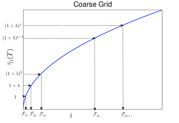
Figure 1: Construction of the coarse-grid set $S_{\lambda}$. The $X$-axis is the class index $i$, and the $Y$-axis represents the corresponding complexity $\overline{\gamma}_{i}(T)$. When the penalty function grows steeply early on, we include a large number of models. The number of complex models included in $S_{\lambda}$ can be significantly smaller as the growth of penalty function tapers out.

If the coarse-grid set is finite and, say, $|S|=s$, then the set $S$ presents a natural collection of indices over which to perform model selection. We simply split the budget uniformly amongst the coarse-grid set $S$, giving budget $T/s$ to each class in the set. Indeed, the main theorem of this section shows that for a large class of problems, it always suffices to restrict our attention to a finite grid set $S$, allowing us to present both a computationally tractable estimator and a good oracle inequality for the estimator. In some cases, there may be no finite coarse grid set. Thus we look for way to restrict our selection to finite sets, which we can do with the following assumption (the assumption is unnecessary if the hierarchy is finite).

Assumption D.

1. There is a constant $B<\infty$ such that $R_{{1}}^{*}\leq B$.

2. For all $n\in\mathbb{N}$ the penalty function $\gamma_{1}(n)\geq 1/n$.

Assumption D(a) is satisfied, for example, if the loss function is bounded, or even if there is a function $f\in\mathcal{F}_{1}$ with finite risk. Assumption D(b) also is mild; unless the class $\mathcal{F}_{1}$ is trivial, in general classes satisfying Assumption C have $\gamma_{1}(n)=\Omega(1/\sqrt{n})$.

Under these assumptions, we provide our computationally budgeted model selection procedure in Algorithm 1. We will see in the proof of Theorem 1 below that the assumptions ensure that we can build a coarse grid of size

$$s=\left\lceil{\log_{2}\left(1+Bn_{1}(T)\right)}\right\rceil+2.$$

In particular, Assumption B(d) ensures that the complexity penalties continue to increase with the class index $i$. Hence, there is a class $K$ such that the complexity penalty $\gamma_{K}$ is larger than the penalized risk of the smallest class $\mathcal{F}_{1}$, at which point no class larger than $K$ can be a minimizer in the oracle inequality. The above choice of $s$ ensures that there is at least one class $j\in S$ so that $j\geq K$, allowing us to restrict our attention only to the function classes $\{\mathcal{F}_{i}\mid i\in S\}$.

0:  Model hierarchy $\{\mathcal{F}_{i}\}$ with corresponding penalty functions $\gamma_{i}$, computational budget $T$, upper bound $B$ on the minimum risk of class 1, and confidence parameter $m$. Construction of the coarse-grid set $S$:

  Set $s=\left\lceil{\log_{2}\left(1+Bn_{1}(T)\right)}\right\rceil+2$.

  for $k=0$ to $s-1$ do

     Set $j_{k+1}$ to be the largest class for which $\overline{\gamma}_{j}(T/s)\leq 2^{k}\overline{\gamma}_{1}(T/s)$.

  end for

  Set $S=\{j_{k}~{}:~{}k=1,\ldots,s\}$. Model selection estimate:

  Set $\hat{f}_{i}=\mathcal{A}\left({i},{T/s}\right)$ for $i\in S$.

  Select a class $\widehat{i}$ that satisfies

$$\widehat{i}\in\mathop{\rm argmin}_{i\in S}\,\left\{\,\widehat{R}_{{n_{i}(T/s)}}(\hat{f}_{i})+\gamma_{i}\left(T/s\right)+\frac{\kappa_{2}}{2}\sqrt{\frac{m}{n_{i}(T/s)}}+\frac{\kappa_{2}}{2}\sqrt{\frac{\log s}{n_{i}(T/s)}}\,\right\}.$$ (10)

  Output the function $f=\hat{f}_{\widehat{i}}=\mathcal{A}\left({\widehat{i}},{T/s}\right)$.

Algorithm 1 Computationally budgeted model selection over nested hierarchies

2.4 Main result and some consequences

With the above definitions in place, we can now provide an oracle inequality on the performance of the model selected by Algorithm 1. We start with our main theorem, and then provide corollaries to help explain various aspects of it.

Theorem 1.

Let $f=\mathcal{A}(\widehat{i},T/s)$ be the output of the algorithm $\mathcal{A}$ for the class $\widehat{i}$ specified by the procedure (10). Let Assumptions A–D be satisfied. With probability at least $1-2\kappa_{1}\exp(-m)$

$$R(f)\leq\min_{i=1,2,3,\ldots}\left\{R_{{i}}^{*}+4\gamma_{i}\left(\frac{T}{s}\right)+\kappa_{2}\sqrt{\frac{8(m+\log s)}{n_{i}(T/s)}}\right\}.$$ (11)

Furthermore, if $n_{1}(T)=\mathcal{O}(T)$ then $s=\mathcal{O}(\log T)$.

The assumption that $n_{1}(T)$ is linear is mild: unless $\mathcal{F}_{1}$ is trivial, any algorithm for $\mathcal{F}_{1}$ must at least observe the data, and hence must use computation at least linear in the sample size.

Remarks:

To better understand the result of Theorem 1, we turn to a few brief remarks.

1. We may ask what an omniscient oracle with access to the same computational algorithm $\mathcal{A}$ could do. Such an oracle would know the optimal class $i^{*}$ and allocate the entire budget $T$ to compute $\mathcal{A}\left({i^{*}},{T}\right)$. By Assumption C, the output $f$ of this oracle satisfies, with probability at least $1-\kappa_{1}\exp(-m)$,

   $$R(f)\leq R_{{i^{*}}}^{*}+\gamma_{i^{*}}(T)+\kappa_{2}\sqrt{\frac{m}{n_{i^{*}}(T)}}=\min_{i=1,2,3,\ldots}\left\{R_{{i}}^{*}+\gamma_{i}(T)+\kappa_{2}\sqrt{\frac{m}{n_{i}(T)}}\right\}.$$ (12)

   Comparing this to the right hand side of the inequality of Theorem 1, we observe that not knowing the optimal class incurs a penalty in the computational budget of roughly a factor of $s$. This penalty is only logarithmic in the computational budget in most settings of interest.

2. Algorithm 1 and Theorem 1, as stated, require a priori knowledge of the computational budget $T$. We can address this using a standard doubling argument (see e.g. [13, Sec. 2.3]). Initially we assume $T=1$ and run Algorithm 1 accordingly. If we do not exhaust the budget, we assume $T=2$, and rerun Algorithm 1 for another round. If there is more computational time at our disposal, we update our guess to $T=4$ and so on. Suppose the real budget is $T_{0}$ with $2^{k}-1<T_{0}\leq 2^{k+1}-1$. After $i$ rounds of this doubling strategy, we have exhausted a budget of $2^{i-1}$, with the last round getting a budget of $2^{i-2}$ for $i\geq 2$. In particular, the last round with a net budget of $T_{0}$ is of length at least $T_{0}/4$. Since Theorem 1 applies to each individual round, we obtain an oracle inequality where we replace $T_{0}$ with $T_{0}/4$; we can be agnostic to the prior knowledge of the budget at the expense of slightly worse constants.

3. For ease of presentation, Algorithm 1 and Theorem 1 use a specific setting of the coarse-grid size, which corresponds to setting $\lambda=1$ in Definition 1. In our proofs, we establish the theorem for arbitrary $\lambda>0$. As a consequence, to obtain slightly sharper bounds, we may optimize this choice of $\lambda$; we do not pursue this here.

Now let us turn to a specialization of Theorem 1 to the settings outlined in Examples 1 and 2. The following corollary shows oracle inequalities under the computational restrictions that are only logarithmically worse than those possible in the computationally unconstrained model selection procedure (3).

Corollary 1.

Let $m\geq 0$ be a specified constant.

1. In the setting of Example 1, define $n$ so that $nT/d$ is the number of samples that can be processed by the inference algorithm $\mathcal{A}$ using $T$ units of computation. Assume that $T$ is large enough that $nT\geq d/B$ and $nT\geq d/(4r_{1}^{2}X^{2})$. With probability at least $1-2\kappa_{1}\exp(-m)$, the output $f$ of Algorithm 1 satisfies

   $$R(f)\leq\inf_{i=1,2,\ldots}\left\{R_{{i}}^{*}+\sqrt{\frac{d\log_{2}(16BnT/d)}{nT}}\left(8r_{i}X+\sqrt{8}\kappa_{2}\sqrt{m+\log\log_{2}(16BnT/d)}\right)\right\}.$$

2. In the setting of Example 2, define $n$ so that $nT/d_{i}$ is the number of samples that can be processed by the inference algorithm $\mathcal{A}$ using $T$ units of computation. Assume that $T$ is large enough that $nT\geq 1$ and $nT\geq d_{1}/B$. With probability at least $1-2\kappa_{1}\exp(-m)$, the output $f$ of Algorithm 1 satisfies

   $$R(f)\leq\inf_{i=1,2,\ldots}\left\{R_{{i}}^{*}+\sqrt{\frac{d_{i}\log_{2}(16BnT/d_{1})}{nT}}\left(4\sqrt{d_{i}}+\sqrt{8}\kappa_{2}\sqrt{m+\log\log_{2}(16BnT/d_{1})}\right)\right\}.$$

2.5 Proofs

As remarked after Theorem 1, we will present our proofs for general settings of $\lambda>0$. For the proofs of Theorem 1 and Corollary 1 in this slight generalization, we define $S_{\lambda}$ as a set satisfying the coarse grid condition with parameters $\lambda$, $m$ and $s(\lambda)$, with $s(\lambda)$ satisfying

$$s(\lambda)\geq\left\lceil{\frac{\log\left(1+\frac{B}{\overline{\gamma}_{1}(T,s(\lambda))}\right)}{\log(1+\lambda)}}\right\rceil+2.$$ (13)

First, we show that this inequality is ensured by the choice given in Algorithm 1. To see this, notice that

$$\left\lceil{\frac{\log\left(1+\frac{B}{\overline{\gamma}_{1}(T,s(\lambda))}\right)}{\log(1+\lambda)}}\right\rceil+2 \leq\left\lceil{\frac{\log\left(1+\frac{B}{\gamma_{1}(T,1)}\right)}{\log(1+\lambda)}}\right\rceil+2$$

$$=\left\lceil{\frac{\log\left(1+Bn_{1}(T)\right)}{\log(1+\lambda)}}\right\rceil+2.$$

Thus, for $\lambda=1$, choosing $s(\lambda)=\left\lceil{\log_{2}\left(1+Bn_{1}(T)\right)}\right\rceil+2$ suffices.

We require the additional notation

$$K(\lambda):=\max\{j~{}:~{}j\in S_{\lambda}\},$$ (14)

where

$$S_{\lambda}=\{j_{1},\ldots,j_{s(\lambda)}\}$$ (15)

is the natural generalization of the set $S$ defined in Algorithm 1: $j_{k+1}$ is chosen as the largest index for which $\overline{\gamma}_{j}(T/s(\lambda))\leq(1+\lambda)^{k}\overline{\gamma}_{1}(T/s(\lambda))$. We begin the proof of Theorem 1 by showing that any $s(\lambda)$ satisfying (13) ensures that any class $j>K(\lambda)$ must have penalty too large to be optimal, so we can focus on classes $j\leq K(\lambda)$. We then show that the output $f$ of Algorithm 1 satisfies an oracle inequality for each class in $S_{\lambda}$, which is possible by an adaptation of arguments in prior work [11]. Using the definition of our coarse grid set (Definition 1), we can then infer an oracle inequality that applies to each class $j\leq K(\lambda)$, and our earlier reduction to a finite model hierarchy completes the argument.

2.5.1 Proof of Theorem 1

First we show that the selection of the set $S_{\lambda}$ satisfies Definition 1.

Lemma 1.

Let $\{\gamma_{i}\}$ be a sequence of increasing positive numbers and for each $k\in\{0,\ldots,s-1\}$ set $j_{k+1}$ to be the largest index $j$ such that $\gamma_{j}\leq(1+\lambda)^{k}\gamma_{1}$. Then for each $i\in\mathbb{N}$ such that $i\leq j_{k}$, there exists a $j\in\{j_{1},\ldots,j_{k}\}$ such that $\gamma_{i}\leq\gamma_{j}\leq(1+\lambda)\gamma_{i}$.

Proof.

Let $i\leq j_{k}$ and choose the smallest $j\in\{j_{1},j_{2},\ldots,j_{k}\}$ such that $\gamma_{i}\leq\gamma_{j}$. Assume for the sake of contradiction that $(1+\lambda)\gamma_{i}<\gamma_{j}$. There exists some $k^{\prime}\in\{0,\ldots,s-1\}$ such that $\gamma_{j}\leq(1+\lambda)^{k^{\prime}}\gamma_{1}$ and $\gamma_{j}\geq(1+\lambda)^{k^{\prime}-1}\gamma_{1}$, and thus we obtain

$$\gamma_{i}<\frac{\gamma_{j}}{1+\lambda}\leq(1+\lambda)^{k^{\prime}-1}\gamma_{1}.$$ (16)

Let $j^{\prime}$ be the largest element smaller than $j$ in the collection $\{j_{1},j_{2},\dots,j_{k}\}$. Then by our construction, $j^{\prime}$ is the largest index satisfying $\gamma_{j^{\prime}}\leq(1+\lambda)^{k^{\prime}-1}\gamma_{1}$. In particular, combining with our earlier inequality (16) leads to the conclusion that $i\leq j^{\prime}$, which contradicts the fact that $j$ is the smallest index in $\{j_{1},\ldots,j_{k}\}$ satisfying $\gamma_{i}\leq\gamma_{j}$. ∎

Next, we show that, for $s(\lambda)$ satisfying (13), once the complexity penalty of a class becomes too large, it can never be the minimizer of the penalized risk in the oracle inequality (11). See Appendix A for the proof.

Lemma 2.

Fix $\lambda>0$ and $m>0$, recall the definition (14) of $K(\lambda)$, and let $i^{*}$ be a class that attains the minimum in the right side of the bound (11). We have $i^{*}\leq K(\lambda)$.

Equipped with the lemmas, we can restrict our attention only to classes $i\in S_{\lambda}$. To that end, the next result establishes an oracle inequality for our algorithm compared to all the classes in this set.

Proposition 1.

Let $f=\hat{f}_{\widehat{i}}$ be the function chosen from the class $\widehat{i}$ selected by the procedure (10), where $S=S_{\lambda}$ and $s=s(\lambda)$. Under the conditions of Theorem 1, with probability at least $1-2\kappa_{1}\exp(-m)$

$$R(f)\leq\min_{i\in S_{\lambda}}\left\{R_{{i}}^{*}+2\gamma_{i}\left(\frac{T}{s(\lambda)}\right)+\kappa_{2}\sqrt{\frac{2(m+\log s(\lambda))}{n_{i}(T/s(\lambda))}}\right\}.$$

The proof of the proposition follows from an argument similar to that given in [11], though we must carefully reason about the different number of independent samples used to estimate within each class $\mathcal{F}_{i}$. We present a proof in Appendix A. We can now complete the proof of Theorem 1 using the proposition.

Proof of Theorem 1:     Let $i$ be any class (not necessarily in $S_{\lambda}$) and $j\in S_{\lambda}$ be the smallest class satisfying $j\geq i$. Then, by construction of $S_{\lambda}$, we know from Lemma 1 that

$$2\gamma_{i}\left(\frac{T}{s(\lambda)}\right)+\kappa_{2}\sqrt{\frac{2(m+\log s(\lambda))}{n_{i}(T/s(\lambda))}} \leq 2\gamma_{j}\left(\frac{T}{s(\lambda)}\right)+\kappa_{2}\sqrt{\frac{2(m+\log s(\lambda))}{n_{j}(T/s(\lambda))}}$$

$$\leq(1+\lambda)\left[2\gamma_{i}\left(\frac{T}{s(\lambda)}\right)+\kappa_{2}\sqrt{\frac{2(m+\log s(\lambda))}{n_{i}(T/s(\lambda))}}\right].$$

In particular, we can lower bound the penalized risk of class $i$ as

$$R_{{i}}^{*}+(1+\lambda)\left[2\gamma_{i}\left(\frac{T}{s(\lambda)}\right)+\kappa_{2}\sqrt{\frac{2(m+\log s(\lambda))}{n_{i}(T/s(\lambda))}}\right]\geq R_{{j}}^{*}+2\gamma_{j}\left(\frac{T}{s(\lambda)}\right)+\kappa_{2}\sqrt{\frac{2(m+\log s(\lambda))}{n_{j}(T/s(\lambda))}},$$

where we used the inclusion assumption A to conclude that $R_{{j}}^{*}\leq R_{{i}}^{*}$. Now applying Proposition 1, the above lower bound, and Lemma 2 in turn, we see that with probability at least $1-2\kappa_{1}\exp(-m)$

$$R(f) \leq\min_{j\in S_{\lambda}}\left\{R_{{j}}^{*}+2\gamma_{j}\left(\frac{T}{s(\lambda)}\right)+\kappa_{2}\sqrt{\frac{2(m+\log s(\lambda))}{n_{j}(T/s(\lambda))}}\right\}$$

$$\leq\min_{i=1,2,\ldots,K(\lambda)}\left\{R_{{i}}^{*}+(1+\lambda)\left(2\gamma_{i}\left(\frac{T}{s(\lambda)}\right)+\kappa_{2}\sqrt{\frac{2(m+\log s(\lambda))}{n_{i}(T/s(\lambda))}}\right)\right\}$$

$$\leq\inf_{i=1,2,3,\ldots}\left\{R_{{i}}^{*}+(1+\lambda)\left(2\gamma_{i}\left(\frac{T}{s(\lambda)}\right)+\kappa_{2}\sqrt{\frac{2(m+\log s(\lambda))}{n_{i}(T/s(\lambda))}}\right)\right\}.$$

For $\lambda=1$ (which we have seen satisfies (13)), this is the desired statement of the theorem. ∎

2.5.2 Proof of Corollary 1

Under the conditions of Example 1, and the assumption that $nT\geq d/(4r_{1}^{2}X^{2})$, Assumptions A-D are satisfied with $n_{i}(T)=nT/d$ and $\gamma_{i}(T)=2r_{i}X\sqrt{d/(nT)}$. (In particular, $nT\geq d/(4r_{1}^{2}X^{2})$ implies that $\gamma_{1}$ satisfies Assumption D(b).) Also, since $nT\geq d/B$, we have

$$s=\left\lceil{\log_{2}\left(1+\frac{BnT}{d}\right)}\right\rceil+2\leq\log_{2}(2BnT/d)+3=\log_{2}(16BnT/d).$$

Substituting into Theorem 1 gives the first part of the corollary.

Similarly, under the conditions of Example 2 and the assumption that $nT\geq 1$, Assumptions A-D are satisfied with $n_{i}(T)=nT/d_{i}$ and $\gamma_{i}(T)=d_{i}/\sqrt{nT}$. (In particular, $nT\geq 1$ implies that $\gamma_{1}$ satisfies Assumption D(b).) Also, since $nT\geq d_{1}/B$, we have $s\leq\log_{2}(16BnT/d)$ as before. Substituting into Theorem 1 gives the second part of the corollary.

3 Fast rates for model selection

Looking at the result given by Theorem 1, we observe that irrespective of the dependence of the penalties $\gamma_{i}$ on the sample size, there are terms in the oracle inequality that always decay as $\mathcal{O}(1/\sqrt{n_{i}(T/s(\lambda))})$. A similar phenomenon is noted in [8] for classical model selection results in computationally unconstrained settings; under conditions similar to Assumption C, this inverse-root dependence on the number of samples is the best possible, due to lower bounds on the fluctuations of the empirical process (e.g. [10, Theorem 2.3]). On the other hand, under suitable low noise conditions [22] or curvature properties of the risk functional [6, 18, 7], it is possible to obtain estimation guarantees of the form

$$R(\hat{f})=R(f^{*})+\mathcal{O}_{p}\left(\frac{1}{n}\right),$$

where $\hat{f}$ (approximately) minimizes the $n$-sample empirical risk. Under suitable assumptions, complexity regularization can also achieve fast rates for model selection [8, 17]. In this section, we show that similar results can be obtained in computationally constrained inferential settings.

3.1 Assumptions and example

We begin by modifying our concentration assumption and providing a motivating example.

Assumption E.

For each $i$, let $f_{i}^{*}\in\mathop{\rm argmin}_{f\in\mathcal{F}_{i}}R(f)$. Then there are constants $\kappa_{1},\kappa_{2}>0$ such that for any budget $T$ and the corresponding sample size $n_{i}(T)$

$$\mathbb{P}\left[\sup_{f\in\mathcal{F}_{i}}\left(R(f)-R(f^{*}_{i})-2(\widehat{R}_{{n_{i}(T)}}(f)-\widehat{R}_{{n_{i}(T)}}(f^{*}_{i}))\right)>\gamma_{i}(T)+\kappa_{2}\epsilon\right]\leq\kappa_{1}\exp(-n_{i}(T)\epsilon).$$ (17a)

$$\mathbb{P}\left[\sup_{f\in\mathcal{F}_{i}}\left(\widehat{R}_{{n_{i}(T)}}(f)-\widehat{R}_{{n_{i}(T)}}(f^{*}_{i})-2(R(f)-R(f^{*}_{i}))\right)>\gamma_{i}(T)+\kappa_{2}\epsilon\right]\leq\kappa_{1}\exp(-n_{i}(T)\epsilon).$$ (17b)

Contrasting this with our earlier Assumption C, we see that the probability bounds (17a) and (17b) decay exponentially in $\epsilon$ rather than $\epsilon^{2}$, which leads to faster sub-exponential rates for estimation procedures. Concentration inequalities of this form are now well known [6, 18, 7], and the paper [8] uses an identical assumption.

Before continuing, we give an example to illustrate the assumption.

Example 3 (Fast rates for classification).

We consider the function class hierarchy based on increasing dimensions of Example 2. We assume that the risk $R(f_{\theta})=\mathbb{E}[\ell(y,f_{\theta}(x))]$ and that the loss function $\ell$ is either the squared loss $\ell(y,f_{\theta}(x))=(y-f_{\theta}(x))^{2}$ or the exponential loss from boosting $\ell(y,f_{\theta}(x))=\exp(-yf_{\theta}(x))$. Each of these examples satisfies Assumption 17 with

$$\gamma_{i}(T)=c\,\frac{d_{i}\log(n_{i}(T)/d_{i})}{n_{i}(T)},$$ (18)

for a universal constant $c$. This follows from Theorem 3 of [8] (which in turn follows from Theorem 3.3 in [6] combined with an argument based on Dudley’s entropy integral [15]). The other parameter settings and computational considerations are identical to those of Example 2.

If we define $\hat{f}_{i}=\mathcal{A}\left({i},{T}\right)$, then using Assumption B(d) (that $\widehat{R}_{{n_{i}(T)}}(\hat{f}_{i})-\widehat{R}_{{n_{i}(T)}}(f^{*}_{i})\leq\gamma_{i}(T)$) in conjunction with Assumption (17a), we can conclude that for any time budget $T$, with probability at least $1-\kappa_{1}\exp(-m)$,

$$R(\hat{f}_{i})\leq R(f^{*}_{i})+3\gamma_{i}(T)+\frac{\kappa_{2}m}{n_{i}(T)}.$$ (19)

One might thus expect that by following arguments similar to those in [8], it would be possible to show fast rates for model selection based on Algorithm 1. Unfortunately, the results of [8] heavily rely on the fact that the data used for computing the estimators $\hat{f}_{i}$ is the same for each class $i$, so that the fluctuations of the empirical processes corresponding to the different classes are positively correlated. In our computationally constrained setting, however, each class’s estimator is computed on a different sample. It is thus more difficult to relate the estimators than in previous work, necessitating a modification of our earlier Algorithm 1 and a new analysis, which follows.

3.2 Algorithm and oracle inequality

As in Section 2, our approach is based on performing model selection over a coarsened version of the collection $\mathcal{F}_{1},\mathcal{F}_{2},\ldots$. To construct the coarser collection of indices, we define the composite penalty term (based on Assumption 17)

$$\overline{\gamma}_{i}(T,s):=20\gamma_{i}\left(\frac{T}{s}\right)+8\frac{\kappa_{2}m+2\log s}{n_{i}(T/s)}.$$ (20)

Based on the above penalty term, we define our analogue of the coarse grid set (9).

We give our modified model selection procedure in Algorithm 2. In the algorithm and in our subsequent analysis, we use the shorthand $\widehat{R}_{{i}}(f)$ to denote the empirical risk of the function $f$ on the $n_{i}(T)$ samples associated with class $i$. Our main oracle inequality is the following:

0:  Model hierarchy $\{\mathcal{F}_{i}\}$ with corresponding penalty functions $\gamma_{i}$, computational budget $T$, upper bound $B$ on the minimum risk of class 1, and confidence parameter $m>0$. Construction of the coarse-grid set $S$:

  Set $s=\left\lceil{\log_{2}\left(1+Bn_{1}(T)\right)}\right\rceil+2$.

  for $k=0$ to $s-1$ do

     Set $j_{k+1}$ to be the largest class for which $\overline{\gamma}_{j}(T/s)\leq 2^{k}\overline{\gamma}_{1}(T/s)$.

  end for

  Set $S=\{j_{k}~{}:~{}k=1,\ldots,s\}$. Model selection estimate:

  Set $\hat{f}_{i}=\mathcal{A}\left({i},{T/s}\right)$ for $i\in S$.

  Select the class $\widehat{i}\in S_{\lambda}$ to be the largest class that satisfies

$$\widehat{R}_{{\widehat{i}}}(\hat{f}_{\widehat{i}})+\frac{17}{2}\gamma_{\widehat{i}}\left(\frac{T}{s}\right)+\frac{9}{2}\kappa_{2}\left(\frac{m+\log s}{n_{\widehat{i}}(T/s)}\right)\leq\widehat{R}_{{\widehat{i}}}(\hat{f}_{j})+\frac{17}{2}\gamma_{j}\left(\frac{T}{s}\right)$$ (21)

for all $j\in S$ such that $j<\widehat{i}$.

  Output the function $\mathcal{A}\left({\widehat{i}},{T/s}\right)$.

Algorithm 2 Computationally budgeted model selection over hierarchies with fast concentration

Theorem 2.

Let $f=\mathcal{A}(\widehat{i},T/s(\lambda))$ be the output of the algorithm $\mathcal{A}$ for class $\widehat{i}$ specified by the procedure (21). Let Assumptions A, B, D and 17 be satisfied. With probability at least $1-2\kappa_{1}\exp(-m)$

$$R(f)\leq\inf_{i=1,2,3,\ldots}\left\{R_{{i}}^{*}+40s\gamma_{i}\left(\frac{T}{s}\right)+10s\kappa_{2}\frac{m+\log s}{n_{i}(T/s)}\right\}.$$ (22)

Furthermore, if $n_{1}(T)=\mathcal{O}(T)$ then $s=\mathcal{O}(\log T)$.

By inspection of the bound (19)—achieved by devoting the full computational budget $T$ to the optimal class—we see that Theorem 2’s oracle inequality has dependence on the computational budget within logarithmic factors of the best possible.

The following corollary shows the application of Theorem 2 to the classification problem we discuss in Example 3.

Corollary 2.

In the setting of Example 3, define $n$ so that $nT/d_{i}$ is the number of samples that can be processed by the inference algorithm $\mathcal{A}$ using $T$ units of computation. Assume that $nT\geq ed_{1}^{2}$, $nT\geq d_{1}/B$, and choose the constant $c$ in the definition (18) of $\gamma_{i}(T)$ such that $c\geq 1/d_{1}$. With probability at least $1-4\kappa_{1}\exp(-m)$, the output $f$ of Algorithm 2 satisfies

$$R(f) \leq\inf_{i=1,2,\ldots}\left\{R_{{i}}^{*}+\frac{10d_{i}\log_{2}^{2}(16BnT/d_{1})}{nT}\left(4cd_{i}\log\left(\frac{nT}{d_{1}^{2}\log_{2}(16BnT/d_{1})}\right)\right.\right.$$

$$\qquad\qquad\qquad\qquad\qquad\qquad\qquad\qquad\left.\left.\rule{0.0pt}{19.91692pt}{}+\kappa_{2}\left(m+\log\log_{2}(16BnT/d_{1})\right)\right)\right\}.$$

3.3 Proofs of main results

In this section, we provide proofs of Theorem 2 and Corollary 2. Like our previous proof for Theorem 1, we again provide the proof of Theorem 2 for general settings of $\lambda>0$. The proof of Theorem 2 broadly follows that of Theorem 1, in that we establish an analogue of Proposition 1, which provides an oracle inequality for each class in the coarse-grid set $S_{\lambda}$. We then extend the proven inequality to apply to each function class $\mathcal{F}_{i}$ in the hierarchy using the definition (9) of the grid set.

Proof of Theorem 2:     Let $n_{i}$ be shorthand for $n_{i}(T/s(\lambda))$, the number of samples available to class $i$, and let $\widehat{R}_{{i}}(f)$ denote the empirical risk of the function $f$ using the $n_{i}$ samples for class $i$. In addition, let $\gamma_{i}(n_{i})$ be shorthand for $\gamma_{i}(n_{i}(T/s(\lambda)))$, the penalty value for class $i$ using $n_{i}(T/s(\lambda))$ samples. With these definitions, we adopt the following shorthand for the events in the probability bounds (17a) and (17b). Let $\epsilon=\{\epsilon_{i}\}$ be an $s(\lambda)$-dimensional vector with (arbitrary for now) positive entries. For each pair of indices $i$ and $j$ define

$$\mathcal{E}_{1}^{ij}\!\left({\epsilon_{i}}\right) :=\bigg{\{}\sup_{f\in\mathcal{F}_{j}}\left(R(f)-R(f^{*}_{j})-2\left(\widehat{R}_{{i}}(f)-\widehat{R}_{{i}}(f^{*}_{j})\right)\right)\leq\gamma_{j}(n_{i})+\kappa_{2}\epsilon_{i}\bigg{\}}$$ (23a)

$$\mathcal{E}_{2}^{ij}\!\left({\epsilon_{i}}\right) :=\bigg{\{}\sup_{f\in\mathcal{F}_{j}}\left(\widehat{R}_{{i}}(f)-\widehat{R}_{{i}}(f^{*}_{j})-2\left(R(f)-R(f^{*}_{j})\right)\right)\leq\gamma_{j}(n_{i})+\kappa_{2}\epsilon_{i}\bigg{\}},$$ (23b)

and define the joint events

$$\mathcal{E}_{1}\!\left({\epsilon}\right):=\bigcup_{i\in S_{\lambda}}\bigcup_{j\in S_{\lambda}}\mathcal{E}_{1}^{ij}\!\left({\epsilon_{i}}\right)~{}~{}~{}\mbox{and}~{}~{}~{}\mathcal{E}_{2}\!\left({\epsilon}\right):=\bigcup_{i\in S_{\lambda}}\bigcup_{j\in S_{\lambda}}\mathcal{E}_{2}^{ij}\!\left({\epsilon_{i}}\right).$$ (24)

With the “good” events (24) defined, we turn to the two technical lemmas, which relate the risk of the chosen function $\hat{f}_{\widehat{i}}$ to $f^{*}_{i}$ for each $i\in S_{\lambda}$. We provide proofs of both lemmas in Appendix B. To make the proofs of each of the lemmas cleaner and see the appropriate choices of constants, we replace the selection strategy (21) with one whose constants have not been specified. Specifically, we select $\widehat{i}$ as the largest class that satisfies

$$\widehat{R}_{{\widehat{i}}}(\hat{f}_{\widehat{i}})+c_{1}\gamma_{\widehat{i}}\left(\frac{T}{s(\lambda)}\right)+c_{2}\kappa_{2}\epsilon_{\widehat{i}}\leq\widehat{R}_{{\widehat{i}}}(\hat{f}_{j})+c_{1}\gamma_{j}\left(\frac{T}{s(\lambda)}\right)$$ (25)

for $j\in S$ with $j\leq\widehat{i}$.

Lemma 3.

Let the events (23a) and (23b) hold for all $i,j\in S_{\lambda}$, that is, $\mathcal{E}_{1}\!\left({\epsilon}\right)$ and $\mathcal{E}_{2}\!\left({\epsilon}\right)$ hold. Then using the selection strategy (25), for each $j\leq\widehat{i}$ with $j\in S_{\lambda}$ we have

$$R(\hat{f}_{\widehat{i}})\leq R(f^{*}_{j})+\frac{1}{2}\left[\left(\frac{17}{2}-c_{1}\right)\gamma_{\widehat{i}}(n_{\widehat{i}})+(6+c_{1})\gamma_{j}(n_{j})+2\kappa_{2}\epsilon_{j}+\left(\frac{9}{2}-c_{2}\right)\kappa_{2}\epsilon_{\widehat{i}}\right].$$

We require a different argument for the case that $j\geq\widehat{i}$, and the constants are somewhat worse.

Lemma 4.

Let the events (23a) and (23b) hold for all $i,j\in S_{\lambda}$, that is, $\mathcal{E}_{1}\!\left({\epsilon}\right)$ and $\mathcal{E}_{2}\!\left({\epsilon}\right)$ hold. Assume also that $c_{1}\geq 17/2$ and $c_{2}\geq 7/2$. Then using the selection strategy (25), for each $j\geq\widehat{i}$ with $j\in S_{\lambda}$ we have

$$R(\hat{f}_{\widehat{i}})\leq R(f^{*}_{j})+s(\lambda)\left[(2c_{1}+3)\gamma_{j}(n_{j})+(2c_{2}+1)\epsilon_{j}\right].$$

We use Lemmas 3 and 4 to complete the proof of the theorem. When Assumption 17 holds, the probability that one of the events $\mathcal{E}_{1}\!\left({\epsilon}\right)$ and $\mathcal{E}_{2}\!\left({\epsilon}\right)$ fails to hold is upper bounded by

$$\mathbb{P}(\mathcal{E}_{1}\!\left({\epsilon}\right)^{c}\cup\mathcal{E}_{2}\!\left({\epsilon}\right)^{c})\leq\sum_{i,j\in S_{\lambda}}\mathbb{P}(\mathcal{E}_{1}^{ij}\!\left({\epsilon_{i}}\right)^{c})+\sum_{i,j\in S_{\lambda}}\mathbb{P}(\mathcal{E}_{2}^{ij}\!\left({\epsilon_{i}}\right)^{c})\leq 2\kappa_{1}\sum_{i,j\in S_{\lambda}}\exp(-n_{i}(T/s(\lambda))\epsilon_{i})$$

by a union bound. Thus, we see that if we define the constants

$$\epsilon_{i}=2\cdot\frac{m+\log(s(\lambda))}{n_{i}(T/s(\lambda))},$$

we obtain that all of the events $\mathcal{E}_{1}^{ij}\!\left({\epsilon_{i}}\right)$ and $\mathcal{E}_{2}^{ij}\!\left({\epsilon_{i}}\right)$ hold with probability at least $1-2\kappa_{1}\exp(-m)$. Applying Lemmas 3 and 4 with the choices $c_{1}=\frac{17}{2}$ and $c_{2}=\frac{9}{2}$, we obtain that with probability at least $1-2\kappa_{1}\exp(-m)$

$$R(\hat{f}_{\widehat{i}})\leq\min_{i\in S_{\lambda}}\left\{R(f^{*}_{i})+s(\lambda)\left(20\gamma_{i}(n_{i})+10\frac{m+\log(s(\lambda))}{n_{i}(T/s(\lambda))}\right)\right\}.$$ (26)

The inequality (26) is the analogue of Proposition 1 in the current setting. Given the inequality, the remainder of the proof of Theorem 2 follows the same recipe as that of Theorem 1. Recalling the notation (14) defining $K(\lambda)$, we apply the inequality (26) with the definition of the grid set (15) to obtain an oracle inequality compared to all classes $i\leq K(\lambda)$. Then provided that

$$s(\lambda)\geq\left\lceil{\frac{\log\left(1+\frac{B}{s(\lambda)\overline{\gamma}_{1}(T,s(\lambda))}\right)}{\log(1+\lambda)}}\right\rceil+2,$$

we can transfer the result to the entire model hierarchy as before. For $\lambda=1$, the choice of $s$ employed in Algorithm 2 again suffices for this. ∎

Proof of Corollary 2:     In the setting of Example 3, we set $n_{i}(T)=nT/d_{i}$ and

$$\gamma_{i}(T)=\frac{cd_{i}\log(n_{i}(T)/d_{i})}{n_{i}(T)}=\frac{cd_{i}^{2}\log(nT/d_{i}^{2})}{nT}.$$

It is straightforward to verify that the conditions of the corollary ensure that Assumptions A, B, D and 17 are satisfied. In particular, $nT\geq ed_{1}^{2}$ and $c\geq 1/d_{1}$ ensure that $\gamma_{1}(T)\geq 1/n_{1}(T)$. Also, $nT\geq d_{1}/B$ ensures that $s\leq\log_{2}(16BnT/d_{1})$. Substituting $\gamma_{i}$, $n_{i}$ and $s$ into Theorem 2 gives the result. ∎

4 Oracle inequalities for unstructured models

To this point, our results have addressed the model selection problem in scenarios where we have a nested collection of models. In the most general case, however, the collection of models may be quite heterogeneous, with no relationship between the different model families. In classification, for instance, we may consider generalized linear models with different link functions, decision trees, random forests, or other families among our collection of models. For a non-parametric regression problem, we may want to select across a collection of dictionaries such as wavelets, splines, and polynomials. While this more general setting is obviously more challenging than the structured cases in the prequel, we would like to study the effects that limiting computation has on model selection problems, understanding when it is possible to outperform computation-agnostic strategies.

4.1 Problem setting and algorithm

When no structure relates the models under consideration, it is impossible to work with an infinite collection of classes within a finite computational time—any estimator must evaluate each class (that is, at least one sample must be allocated to each class, as any class could be significantly better than the others). As a result, we restrict ourselves to finite model collections in this section, so that we have a sequence $\mathcal{F}_{1},\dots,\mathcal{F}_{K}$ of models from which we wish to select. Our approach to the unstructured case is to incrementally allocate computational quota amongst the function classes, where we trade off receiving samples for classes that have good risk performance against exploring classes for which we have received few data points. More formally, with $T$ available quanta of computation, it is natural to view the model selection problem as a $T$ round game, where in each round a procedure selects a function class $i$ and allocates it one additional quantum of computation.

With this setup, we turn to stating a few natural assumptions. We assume that the computational complexity of fitting a model grows linearly and incrementally with the number of samples, which means that allocating an additional quantum of training time allows the learning algorithm $\mathcal{A}$ to process an additional $n_{i}$ samples for class $\mathcal{F}_{i}$. In the context of Sections 2 and 3, this means that we assume $n_{i}(t)=tn_{i}$ for some fixed number $n_{i}$ specific to class $i$. This linear growth assumption is satisfied, for instance, when the loss function $\ell$ is convex and the black-box learning algorithm $\mathcal{A}$ is a stochastic or online convex optimization procedure [13, 24]. We also require assumptions similar to Assumptions B and C:

Assumption F.

Let $\mathcal{A}\left({i},{T}\right)\in\mathcal{F}_{i}$ denote the output of algorithm $\mathcal{A}$ when executed for class $\mathcal{F}_{i}$ with a computational budget $T$.

1. For each $i$, there exists an $n_{i}\in\mathbb{N}$ such that in $T$ units of time, algorithm $\mathcal{A}$ can compute $\mathcal{A}\left({i},{T}\right)$ using $n_{i}T$ samples.

2. For each $i\in[K]$, there is a function $\gamma_{i}$ and constants $\kappa_{1},\kappa_{2}>0$ such that for any $T\in\mathbb{N}$,

   $$\mathbb{P}\left(|\widehat{R}_{{n_{i}T}}(\mathcal{A}\left({i},{T}\right))-R(\mathcal{A}\left({i},{T}\right))|>\gamma_{i}(n_{i}T)+\kappa_{2}\epsilon\right)\leq\kappa_{1}\exp(-4n_{i}T\epsilon^{2}).$$ (27)

3. The output $\mathcal{A}\left({i},{T}\right)$ is a $\gamma_{i}(n_{i}T)$-minimizer of $\widehat{R}_{{n_{i}T}}$, that is,

   $$\widehat{R}_{{n_{i}T}}(\mathcal{A}\left({i},{n_{i}T}\right))-\inf_{f\in\mathcal{F}_{i}}\widehat{R}_{{n_{i}T}}(f)\leq\gamma_{i}(n_{i}T).$$

4. For each $i$, the function $\gamma_{i}$ satisfies $\gamma_{i}(n)\leq c_{i}n^{-\alpha_{i}}$ for some $\alpha_{i}>0$.

5. For any fixed function $f\in\mathcal{F}_{i}$, $\mathbb{P}(|\widehat{R}_{{n}}(f)-R(f)|>\kappa_{2}\epsilon)\leq\kappa_{1}\exp(-4n\epsilon^{2})$.

Comparing to Assumptions B and C, we see that the main difference is in the linear time assumption (a) and growth assumption (d). In addition, the complexity penalties and function classes discussed in our earlier examples satisfy Assumption F.

We now present our algorithm for successively allocating computational quanta to the function classes. To choose the class $i$ receiving computation at iteration $t$, the procedure must balance competing goals of exploration, evaluating each function class $\mathcal{F}_{i}$ adequately, and exploitation, giving more computation to classes with low empirical risk. To promote exploration, we use an optimistic selection criterion to choose class $i$, which—assuming that $\mathcal{F}_{i}$ has seen $n$ samples at this point—is

$$\overline{R}(i,n)=\widehat{R}_{{n}}(\mathcal{A}\left({i},{n}\right))-\gamma_{i}(n)-\sqrt{\frac{\log K}{n}}+\gamma_{i}(Tn_{i}).$$ (28)

The intuition behind the definition of $\overline{R}(i,n)$ is that we would like the algorithm to choose functions $f$ and classes $i$ that minimize $\widehat{R}_{{n}}(f)+\gamma_{i}(Tn_{i})\approx R(f)+\gamma_{i}(Tn_{i})$, but the negative $\gamma_{i}(n)$ and $\sqrt{\log K/n}$ terms lower the criterion significantly when $n$ is small and thus encourage initial exploration. The criterion (28) essentially combines a penalized model-selection objective with an optimistic criterion similar to those used in multi-armed bandit algorithms [2]. Algorithm 3 contains the formal description of our bandit procedure for model selection. Algorithm 3 begins by receiving $n_{i}$ samples for each of the $K$ classes $\mathcal{F}_{i}$ to form the preliminary empirical estimates (28); we then use the optimistic selection criterion until the computational budget is exhausted.

  For each $i\in[K]$, query $n_{i}$ examples from class $\mathcal{F}_{i}$.

  for $t=K+1$ to $T$ do

     Let $n_{i}(t)$ be the number of examples seen for class $i$ until time $t$

     Let $i_{t}=\mathop{\rm argmin}_{i\in[K]}\overline{R}(j,n_{i}(t))-\sqrt{\frac{\log t}{n_{i}(t)}}$.

     Query $n_{i_{t}}$ examples for class $i_{t}$.

  end for

  Output $\widehat{i}$, the index of the most frequently queried class.

Algorithm 3 Multi-armed bandit algorithm for selection of best class $\widehat{i}$.

4.2 Main results and some consequences

The goal of the selection procedure is to find the best penalized class ${i^{*}}$: a class satisfying

$${i^{*}}\in\mathop{\rm argmin}_{i\in[K]}\left\{\inf_{f\in\mathcal{F}_{i}}R(f)+\gamma_{i}(Tn_{i})\right\}=\mathop{\rm argmin}_{i\in[K]}\left\{R_{{i}}^{*}+\gamma_{i}(Tn_{i})\right\}.$$

To present our main results for Algorithm 3, we define the excess penalized risk $\Delta_{i}$ of class $i$:

$$\Delta_{i}:=R_{{i}}^{*}+\gamma_{i}(Tn_{i})-R_{{{i^{*}}}}^{*}-\gamma_{{i^{*}}}(Tn_{{i^{*}}})\geq 0.$$ (29)

Without loss of generality, we assume that the infimum in $R_{{i}}^{*}=\inf_{f\in\mathcal{F}_{i}}R(f)$ is attained by a function $f_{i}^{*}$ (if not, we use a limiting argument, choosing some fixed $f_{i}^{*}$ such that $R(f_{i}^{*})\leq\inf_{f\in\mathcal{F}_{i}}R(f)+\delta$ for an arbitrarily small $\delta>0$).

The gains of a computationally adaptive strategy over naïve strategies are clearest when the gap (29) is non-zero for each $i$, though in the sequel, we forgo this requirement. Under this assumption, we can follow the ideas of Auer et al. [2] to show that the fraction of the computational budget allocated to any suboptimal class $i\neq{i^{*}}$ goes quickly to zero as $T$ grows. We provide the proof of the following theorem in Section 4.3.

Theorem 3.

Let Alg. 3 be run for $T$ rounds, and let $T_{i}(t)$ be the number of times class $i$ is queried through round $t$. Let $\Delta_{i}$ be defined as in (29) and Assumption F hold, and assume that $T\geq K$. Define $\beta_{i}=\max\{1/\alpha_{i},2\}$. There is a constant $C$ such that

$$\mathbb{E}[T_{i}(T)]\leq\frac{C}{n_{i}}\left(\frac{c_{i}+\kappa_{2}\sqrt{\log T}}{\Delta_{i}}\right)^{\beta_{i}}~{}~{}~{}\mbox{and}~{}~{}~{}\mathbb{P}\left(T_{i}(T)>\frac{C}{n_{i}}\left(\frac{c_{i}+\kappa_{2}\sqrt{\log T}}{\Delta_{i}}\right)^{\beta_{i}}\right)\leq\frac{\kappa_{1}}{TK^{4}},$$

where $c_{i}$ and $\alpha_{i}$ are the constants in the definition F(d) of the concentration function $\gamma_{i}$.

At a high level, this result shows that the fraction of budget allocated to any suboptimal class goes to 0 at the rate $\frac{1}{n_{i}T}\left(\frac{\sqrt{\log T}}{\Delta_{i}}\right)^{\beta_{i}}$. Hence, asymptotically in $T$, the procedure performs almost as if all the computational budget were allocated to class ${i^{*}}$. To see an example of concrete rates that can be concluded from the above result, let $\mathcal{F}_{1},\dots,\mathcal{F}_{K}$ be model classes with finite VC-dimension, so that Assumption F is satisfied with $\alpha_{i}=\frac{1}{2}$. Then we have

Corollary 3.

Under the conditions of Theorem 3, assume $\mathcal{F}_{1},\dots,\mathcal{F}_{K}$ are model classes of finite VC-dimension, where $\mathcal{F}_{i}$ has dimension $d_{i}$. Then there is a constant $C$ such that

$$\mathbb{E}[T_{i}(T)]\leq C\frac{\max\{d_{i},\kappa_{2}^{2}\log T\}}{\Delta^{2}_{i}n_{i}}~{}~{}~{}\mbox{and}~{}~{}~{}\mathbb{P}\left(T_{i}(T)>C\frac{\max\{d_{i},\kappa_{2}^{2}\log T\}}{\Delta^{2}_{i}n_{i}}\right)\leq\frac{\kappa_{1}}{TK^{4}}.$$

A lower bound by Lai and Robbins [19] for the multi-armed bandit problem shows that Corollary 3 is nearly optimal in general. To see the connection, let $\mathcal{F}_{i}$ correspond to the $i$th arm in a multi-armed bandit problem and the risk $R_{{i}}^{*}$ be the expected reward of arm $i$ and assume w.l.o.g. that $R_{{i}}^{*}\in[0,1]$. In this case, the complexity penalty $\gamma_{i}$ for each class is 0. Let $p_{i}$ be a distribution on $\{0,1\}$, where $p_{i}(1)=R_{{i}}^{*}$ and $p_{i}(0)=1-R_{{i}}^{*}$ (let $p_{i}=p_{i}(1)$ for shorthand). Lai and Robbins give a lower bound that shows that the expected number of pulls of any suboptimal arm is at least $\mathbb{E}[T_{i}(T)]=\Omega\left(\log T/\mathop{\rm KL}\left({p_{i}}|\!|{p_{{i^{*}}}}\right)\right)$, where $p_{i}$ and $p_{{i^{*}}}$ are the reward distributions for the $i$th and optimal arms, respectively. An asymptotic expansion shows that $\mathop{\rm KL}\left({p_{i}}|\!|{p_{{i^{*}}}}\right)=\Delta_{i}^{2}/(2p_{i}(1-p_{i}))$, plus higher order terms, in this case; Corollary 3 is essentially tight.

The condition that the gap $\Delta_{i}>0$ may not always be satisfied, or $\Delta_{i}$ may be so small as to render the bound in Theorem 3 vacuous. Nevertheless, it is intuitive that our algorithm can quickly find a small set of “good” classes—those with small penalized risk—and spend its computational budget to try to distinguish amongst them. In this case, Algorithm 3 does not visit suboptimal classes and so can output a function $f$ satisfying good oracle bounds. In order to prove a result quantifying this intuition, we first upper bound the regret of Algorithm 3, that is, the average excess risk suffered by the algorithm over all iterations, and then show how to use this bound for obtaining a model with a small risk. For the remainder of the section, we simplify the presentation by assuming that $\alpha_{i}\equiv\alpha$ and define $\beta=\max\{1/\alpha,2\}$.

Proposition 2.

Use the same assumptions as Theorem 3, but further assume that $\alpha_{i}\equiv\alpha$ for all $i$. With probability at least $1-\kappa_{1}/TK^{3}$, the regret (average excess risk) of Algorithm 3 satisfies

$$\sum_{i=1}^{K}\Delta_{i}T_{i}(T)\leq 2eT^{1-1/\beta}\left(C\sum_{i=1}^{K}\frac{(c_{i}+\kappa_{2}\sqrt{\log T})^{\beta}}{n_{i}}\right)^{1/\beta}$$

for a constant $C$ dependent on $\alpha$.

Our final main result builds on Proposition 2 to show that when it is possible to average functions across classes $\mathcal{F}_{i}$, we can aggregate all the “played” functions $f_{t}$, one for each iteration $t$, to obtain a function with small risk. Indeed, setting $f_{t}=\mathcal{A}\left({i_{t}},{n_{i_{t}}(t)}\right)$, we obtain the following theorem (whose proof, along with that of Proposition 2, we provide in Appendix D):

Theorem 4.

Use the conditions of Proposition 2. Let the risk function $R$ be convex on $\mathcal{F}_{1}\cup\ldots\cup\mathcal{F}_{K}$, and let $f_{t}$ be the function chosen by algorithm $\mathcal{A}$ at round $t$ of Alg. 3. Define the average function $\widehat{f}_{T}=\frac{1}{T}\sum_{t=1}^{T}f_{t}$. There are constants $C$, $C^{\prime}$ (dependent on $\alpha$) such that with probability greater than $1-2\kappa_{2}/(TK^{3})$,

$$R(\widehat{f}_{T}) \leq R^{*}+\gamma_{i^{*}}(Tn_{i^{*}})+2e\kappa_{2}T^{-\beta}\sqrt{\log T}\left(\sum_{i=1}^{K}\frac{C}{n_{i}}\right)^{1/\beta}$$

$$\quad~{}+C^{\prime}\,T^{-1/\beta}\left(\sum_{i=1}^{K}\left[c_{i}n_{i}^{-\alpha}+\kappa_{2}n_{i}^{-\frac{1}{2}}\sqrt{\log K}+\kappa_{2}n_{i}^{-\frac{1}{2}}\sqrt{\log T}\right]^{\beta}\right)^{1/\beta}.$$

Let us interpret the above bound and discuss its optimality. When $\alpha=\frac{1}{2}$ (e.g., for VC classes), we have $\beta=2$; moreover, it is clear that $\sum_{i=1}^{K}\frac{C}{n_{i}}=\mathcal{O}(K)$. Thus, to within constant factors,

$$R(\widehat{f}_{T})=R_{{{i^{*}}}}^{*}+\gamma_{{i^{*}}}(Tn_{{i^{*}}})+\mathcal{O}\left(\frac{\sqrt{K\max\{\log T,\log K\}}}{\sqrt{T}}\right).$$

Ignoring logarithmic factors, the above bound is minimax optimal, which follows by a reduction of our model selection problem to the special case of a multi-armed bandit problem. In this case, Theorem 5.1 of Auer et al. [3] shows that for any set of $K,T$ values, there is a distribution over the rewards of arms which forces $\Omega(\sqrt{KT})$ regret, that is, the average excess risk of the classes chosen by Alg. 3 must be $\Omega(\sqrt{KT})$, matching Proposition 2 and Theorem 4.

The scaling $\mathcal{O}(\sqrt{K})$ is essentially as bad as splitting the computational budget $T$ uniformly across each of the $K$ classes, which yields (roughly) an oracle inequality of the form

$$R(f)=R_{{{i^{*}}}}^{*}+\gamma_{i^{*}}(Tn_{i^{*}}/K)+\mathcal{O}\bigg{(}\frac{\sqrt{K\log K}}{\sqrt{Tn_{i^{*}}}}\bigg{)}.$$

Comparing this bound to Theorem 4, we see that the penalty $\gamma_{i}$ in the theorem is smaller. The other key distinction between the two bounds (ignoring logarithmic factors) is the difference between

$$\sum_{i=1}^{K}\frac{1}{n_{i}}~{}~{}\mbox{and}~{}~{}\frac{K}{n_{i^{*}}}.$$

When the left quantity is smaller than the right, the bandit-based Algorithm 3 and the extension indicated by Theorem 4 give improvements over the naïve strategy of uniformly splitting the budget across classes. However, if each class has similar computational cost $n_{i}$, no strategy can outperform the naïve one.

We also observe that we can apply the online procedure of Algorithm 3 to the nested setup of Sections 2 and 3 as well. In this case, by applying Algorithm 3 only to elements of the coarse-grid set $S_{\lambda}$, we can replace $K$ in the bounds of Theorems 3 and 4 with $s(\lambda)$, which gives results similar to our earlier Theorems 1 and 2. In particular, if we are in the setup of Theorem 3 with a large separation between penalized risks, then Algorithm 3 applied to the coarse-grid set is expected to outperform a uniform allocation of budget within the set as in Sections 2 and 3.

4.3 Proof of Theorem 3

At a high level, the proof of this theorem involves combining the techniques for analysis of multi-armed bandits developed by Auer et al. [2] with Assumption F. We start by giving a lemma that will be useful to prove the theorem. The lemma states that after a sufficient number of initial iterations $\tau$, the probability that Algorithm 3 chooses to receive samples for a sub-optimal function class $i\neq{i^{*}}$ is extremely small. Recall also our notational convention that $\beta_{i}=\max\{1/\alpha_{i},2\}$.

Lemma 5.

Let Assumption F hold. For any class $i$, any $s_{i}\in[1,T]$ and $s_{{i^{*}}}\in[\tau,T]$ where $\tau$ satisfies

$$\tau>\frac{2^{\beta_{i}}(c_{i}+\kappa_{2}\sqrt{\log T}+\kappa_{2}\sqrt{\log K})^{\beta_{i}}}{n_{i}\Delta_{i}^{\beta_{i}}},$$

we have

$$\mathbb{P}\left(\overline{R}(i,n_{i}s_{i})-\kappa_{2}\sqrt{\frac{\log T}{n_{i}s_{i}}}\leq\overline{R}({i^{*}},n_{i^{*}}s_{i^{*}})-\kappa_{2}\sqrt{\frac{\log T}{n_{{i^{*}}}s_{{i^{*}}}}}\right)\leq\frac{2\kappa_{1}}{(TK)^{4}}.$$

We defer the proof of the lemma to Appendix C, though at a high level the proof works as follows. The “bad event” in Lemma 5, which corresponds to Algorithm 3 selecting a sub-optimal class $i\neq{i^{*}}$, occurs only if one of the following three errors occurs: the empirical risk of class $i$ is much lower than its true risk, the empirical risk of class ${i^{*}}$ is higher than its true risk, or $s_{i}$ is not large enough to actually separate the true penalized risks from one another. The assumptions of the lemma make each of these three sub-events quite unlikely. Now we turn to the proof of Theorem 3, assuming the lemma.

Let $i_{t}$ denote the model class index $i$ chosen by Algorithm 3 at time $t$, and let $s_{i}(t)$ denote the number of times class $i$ has been selected at round $t$ of the algorithm. When no time index is needed, $s_{i}$ will denote the same thing. Note that if $i_{t}=i$ and the number of times class $i$ is queried exceeds $\tau>0$, then by the definition of the selection criterion (28) and choice of $i_{t}$ in Alg. 3, for some $s_{i}\in\{\tau,\ldots,t-1\}$ and $s_{{i^{*}}}\in\{1,\ldots,t-1\}$ we have

$$\overline{R}(i,n_{i}s_{i})-\kappa_{2}\sqrt{\frac{\log T}{n_{i}s_{i}}}\leq\overline{R}({i^{*}},n_{i^{*}}s_{i^{*}})-\kappa_{2}\sqrt{\frac{\log T}{n_{i^{*}}s_{i^{*}}}}.$$

Here we interpret $\overline{R}(i,n_{i}s_{i})$ to mean a random realization of the observed risk consistent with the samples we observe. Using the above implication, we thus have

$$T_{i}(T) =1+\sum_{t=K+1}^{T}\mathbb{I}\left({i_{t}=i}\right)~{}~{}\leq~{}~{}\tau+\sum_{t=K+1}^{T}\mathbb{I}\left({i_{t}=i,T_{i}(t-1)\geq\tau}\right)$$

$$\leq\tau+\sum_{t=K+1}^{T}\mathbb{I}\left({\min_{\tau\leq s_{i}<t}\overline{R}(i,n_{i}s_{i})-\kappa_{2}\sqrt{\frac{\log T}{n_{i}s_{i}}}\leq\max_{0<s<t}\overline{R}({i^{*}},n_{i^{*}}s_{i^{*}})-\kappa_{2}\sqrt{\frac{\log T}{n_{{i^{*}}}s_{{i^{*}}}}}}\right)$$

$$\leq\tau+\sum_{t=1}^{T}\sum_{s_{i^{*}}=1}^{t-1}\sum_{s_{i}=\tau}^{t-1}\mathbb{I}\left({\overline{R}(i,n_{i}s_{i})-\kappa_{2}\sqrt{\frac{\log T}{n_{i}s_{i}}}\leq\overline{R}({i^{*}},n_{i^{*}}s_{i^{*}})-\kappa_{2}\sqrt{\frac{\log T}{n_{{i^{*}}}s_{{i^{*}}}}}}\right).$$ (30)

To control the last term, we invoke Lemma 5 and obtain that

$$\tau>\frac{2^{\beta_{i}}(c_{i}+\kappa_{2}\sqrt{\log T}+\kappa_{2}\sqrt{\log K})^{\beta_{i}}}{n_{i}\Delta_{i}^{\beta_{i}}}~{}~{}\Rightarrow~{}~{}\mathbb{E}[T_{i}(T)]\leq\tau+\sum_{t=1}^{T}\sum_{s=1}^{t-1}\sum_{s_{i}=\tau}^{t-1}2\frac{\kappa_{1}}{(TK)^{4}}\leq\tau+\frac{\kappa_{1}}{TK^{4}}.$$

Hence for any suboptimal class $i\neq{i^{*}}$, $\mathbb{E}[T_{i}(n)]\leq\tau_{i}+\kappa_{1}/(TK^{4})$, where $\tau_{i}$ satisfies the lower bound of Lemma 5 and is thus logarithmic in $T$. Under the assumption that $T\geq K$, for $i\neq{i^{*}}$,

$$\mathbb{E}[T_{i}(T)]\leq C\frac{(c_{i}+\kappa_{2}\sqrt{\log T})^{\max\{1/\alpha_{i},2\}}}{n_{i}\Delta_{i}^{\max\{1/\alpha_{i},2\}}}$$ (31)

for a constant $C\leq 2\cdot 4^{\max\{1/\alpha_{i},2\}}$. Now we prove the high-probability bound. For this part, we need only concern ourselves with the sum of indicators from (30). Markov’s inequality shows that

$$\mathbb{P}\left(\sum_{t=K+1}^{T}\mathbb{I}\left({i_{t}=i,T_{i}(t-1)\geq\tau}\right)\geq 1\right)\leq\frac{\kappa_{1}}{TK^{4}}.$$

Thus we can assert that the bound (31) on $T_{i}(T)$ holds with high probability.

Remark:

By examining the proof of Theorem 3, it is straightforward to see that if we modify the multipliers on the square root terms in the criterion (28) by $m\kappa_{2}$ instead of $\kappa_{2}$, we get that the probability bound is of the order $T^{3-4m^{2}}K^{-4m^{2}}$, while the bound on $T_{i}(T)$ is scaled by $m^{1/\alpha_{i}}$.

5 Discussion

In this paper, we have presented a new framework for model selection with computational constraints. The novelty of our setting is the idea of using computation—rather than samples—as the quantity against which we measure the performance of our estimators. As our main contribution, we have presented algorithms for model selection in several scenarios, and the common thread in each is that we attain good performance by evaluating only a small and intelligently-selected set of models, allocating samples to each model based on computational cost. For model selection over nested hierarchies, this takes the form of a new estimator based on a coarse gridding of the model space, which is competitive (up to logarithmic factors) with an omniscient oracle. A minor extension of our algorithm is adaptive to problem complexity, since it yields fast rates for model selection when the underlying estimation problems have appropriate curvature or low-noise properties. We also presented an exploration-exploitation algorithm for model selection in unstructured cases, showing that it obtains (in some sense) nearly optimal performance.

There are certainly many possible extensions and open questions that our work raises. We address the setting where the complexity penalties are known and can be computed easily in closed form. Often it is desirable to use data-dependent penalties [20, 6, 23], since they adapt to the particular problem instance and data distribution. It appears to be somewhat difficult to extend such penalties to the procedures we have developed in this paper, but we believe it would be quite interesting. Another natural question to ask is whether there exist intermediate model selection problems between a nested sequence of classes and a completely unstructured collection. Identifying other structures—and obtaining the corresponding oracle inequalities and understanding their dependence on computation—would be an interesting extension of the results presented here.

More broadly, we believe the idea of using computation, in addition to the number of samples available for a statistical inference problem, to measure the performance of statistical procedures is appealling for a much broader class of problems. In large data settings, one would hope that more data would always improve the risk performance of statistical procedures, even with a fixed computational budget. We hope that extending these ideas to other problems, and understanding how computation interacts with and affects the quality of statistical estimation more generally, will be quite fruitful.

Appendix A Auxiliary results for Theorem 1 and Corollary 1

We start by establishing Lemma 2. To prove the lemma, we first need a simple claim.

Lemma 6.

Let $c_{1}>c_{2}>0$, $s>0$, and define

$$i_{1}^{*} =\mathop{\rm argmin}_{i=1,2,3,\ldots}\left\{R_{{i}}^{*}+c_{1}\left(\gamma_{i}\left(\frac{T}{s}\right)+\kappa_{2}\sqrt{\frac{2(m+\log s)}{n_{i}(T/s)}}\right)\right\},$$

$$i_{2}^{*} =\mathop{\rm argmin}_{i=1,2,3,\ldots}\left\{R_{{i}}^{*}+c_{2}\left(\gamma_{i}\left(\frac{T}{s}\right)+\kappa_{2}\sqrt{\frac{2(m+\log s)}{n_{i}(T/s)}}\right)\right\}.$$

Then under the monotonicity assumptions B, we have $i_{1}^{*}\leq i_{2}^{*}$.

Proof.

Recall the shorthand definition (8) of $\overline{\gamma}_{i}$. Under the monotonicity assumptions B(a)–(b), $\overline{\gamma}_{i}$ is monotone increasing in $i$. By the definitions of $i_{1}^{*}$ and $i_{2}^{*}$ we have

$$R_{{i_{1}}}^{*}+c_{1}\overline{\gamma}_{i_{1}^{*}}\left(T,s\right)\leq R_{{i_{2}}}^{*}+c_{1}\overline{\gamma}_{i_{2}^{*}}\left(T,s\right)~{}~{}~{}\mbox{and}~{}~{}~{}R_{{i_{2}}}^{*}+c_{2}\overline{\gamma}_{i_{2}^{*}}\left(T,s\right)\leq R_{{i_{1}}}^{*}+c_{2}\overline{\gamma}_{i_{1}^{*}}\left(T,s\right).$$

Adding the two inequalities we obtain

$$(c_{1}-c_{2})\overline{\gamma}_{i_{1}^{*}}\left(T,s\right)\leq(c_{1}-c_{2})\overline{\gamma}_{i_{2}^{*}}\left(T,s\right).$$

Since $c_{1}-c_{2}>0$ by assumption, the monotonicity of $\overline{\gamma}_{i}$ guarantees $i_{1}^{*}\leq i_{2}^{*}$. ∎

Proof of Lemma 2:     Lemma 6 allows us to establish a simpler version of Lemma 2. Since $1+\lambda>1$, it suffices to establish $i_{0}\leq K(\lambda)$, where

$$i_{0}=\mathop{\rm argmin}_{i=1,2,3,\ldots}\left\{R_{{i}}^{*}+\gamma_{i}\left(\frac{T}{s(\lambda)}\right)+\kappa_{2}\sqrt{\frac{2(m+\log s(\lambda))}{n_{i}(T/s(\lambda))}}\right\}.$$

Let $\overline{\gamma}_{i}$ be shorthand for the quantity (8) as usual. Recalling the construction of $S_{\lambda}$ in (15), we observe that any class $i>K(\lambda)$ satisfies

$$(1+\lambda)^{s(\lambda)-2}\,\overline{\gamma}_{1}\left(T,s(\lambda)\right)<\overline{\gamma}_{i}\left(T,s(\lambda)\right)$$

The setting (13) of $s(\lambda)$ ensures that

$$(1+\lambda)^{s(\lambda)-2}\geq(1+\lambda)^{\left\lceil{\log(1+B/\overline{\gamma}_{1}(T,s(\lambda)))/\log(1+\lambda)}\right\rceil}\geq\exp\left(\log\left(1+\frac{B}{\overline{\gamma}_{1}(T,s(\lambda))}\right)\right)$$

so that

$$(1+\lambda)^{s(\lambda)-2}\,\overline{\gamma}_{1}\left(T,s(\lambda)\right)\geq B+\overline{\gamma}_{1}\left(T,s(\lambda)\right)\geq R_{{1}}^{*}+\overline{\gamma}_{1}\left(T,s(\lambda)\right)\geq\inf_{i}\left\{R_{{i}}^{*}+\overline{\gamma}_{i}\left(T,s(\lambda)\right)\right\}.$$

Hence we observe that for $i>K(\lambda)$,

$$R_{{i}}^{*}+\overline{\gamma}_{i}\left(T,s(\lambda)\right) \geq\overline{\gamma}_{i}\left(T,s(\lambda)\right)$$

$$>(1+\lambda)^{s(\lambda)-2}\,\overline{\gamma}_{1}\left(T,s(\lambda)\right)$$

$$\geq\inf_{j\in\{1,2,\ldots\}}\left\{R_{{j}}^{*}+\overline{\gamma}_{j}\left(T,s(\lambda)\right)\right\}.$$

We must thus have $i_{0}\leq K(\lambda)$, and Lemma 6 further implies that $i^{*}\leq K(\lambda)$. ∎

We finally provide a proof for Proposition 1.

Proof of Proposition 1:     Since for any $a,b\geq 0$, $\sqrt{a}+\sqrt{b}\leq\sqrt{2(a+b)}$, it suffices to control the probability of the event

$$R(f)>\min_{i\in S}\bigg{\{}R_{{i}}^{*}+2\gamma_{i}\left(\frac{T}{s(\lambda)}\right)+\kappa_{2}\sqrt{\frac{\log s(\lambda)}{n_{i}(T/s(\lambda))}}+\kappa_{2}\sqrt{\frac{m}{n_{i}(T/s(\lambda))}}\bigg{\}}.$$ (32)

For the event (32) to occur, at least one of

$$R(f)>\min_{i\in S}\left\{\widehat{R}_{{n_{i}(T/s(\lambda))}}(\hat{f}_{i})+\gamma_{i}\left(\frac{T}{s(\lambda)}\right)+\frac{\kappa_{2}}{2}\sqrt{\frac{m}{n_{i}(T/s(\lambda))}}+\frac{\kappa_{2}}{2}\sqrt{\frac{\log s(\lambda)}{n_{i}(T/s(\lambda))}}\right\}$$ (33a)

or

$$\min_{i\in S}\left\{\widehat{R}_{{n_{i}(T/s(\lambda))}}(\hat{f}_{i})+\gamma_{i}\left(\frac{T}{s(\lambda)}\right)+\frac{\kappa_{2}}{2}\sqrt{\frac{\log s(\lambda)}{n_{i}(T/s(\lambda))}}+\frac{\kappa_{2}}{2}\sqrt{\frac{m}{n_{i}(T/s(\lambda))}}\right\}$$

$$\qquad~{}>\min_{i\in S}\left\{R_{{i}}^{*}+2\gamma_{i}\left(\frac{T}{s(\lambda)}\right)+\kappa_{2}\sqrt{\frac{\log s(\lambda)}{n_{i}(T/s(\lambda))}}+\kappa_{2}\sqrt{\frac{m}{n_{i}(T/s(\lambda))}}\right\}$$ (33b)

must occur.

We bound the probabilities of the events (33a) and (33b) in turn.

If the event (33a) occurs, by definition of the selection strategy (10), it must be the case that for some $i\in S$ (namely $i=\widehat{i}$)

$$R(\hat{f}_{i})>\widehat{R}_{{n_{i}(T/s(\lambda))}}(\hat{f}_{i})+\gamma_{i}\left(\frac{T}{s(\lambda)}\right)+\frac{\kappa_{2}}{2}\sqrt{\frac{m}{n_{i}(T/s(\lambda))}}+\frac{\kappa_{2}}{2}\sqrt{\frac{\log s(\lambda)}{n_{i}(T/s(\lambda))}}$$

since the chosen $f$ minimizes the right side of this display over the classes $\mathcal{F}_{i}$ for $i\in S$. By a union bound, we see that

$$\mathbb{P}\left[R(f)>\min_{i\in S}\left\{\widehat{R}_{{n_{i}(T/s(\lambda))}}(\hat{f}_{i})+\gamma_{i}\left(\frac{T}{s(\lambda)}\right)+\frac{\kappa_{2}}{2}\sqrt{\frac{m}{n_{i}(T/s(\lambda))}}+\frac{\kappa_{2}}{2}\sqrt{\frac{\log s(\lambda)}{n_{i}(T/s(\lambda))}}\right\}\right]$$

$$\leq\mathbb{P}\left[\exists~{}i\in S~{}\mbox{s.t.}~{}R(\hat{f}_{i})>\widehat{R}(\hat{f}_{i})+\gamma_{i}\left(\frac{T}{s(\lambda)}\right)+\frac{\kappa_{2}}{2}\sqrt{\frac{m}{n_{i}(T/s(\lambda))}}+\frac{\kappa_{2}}{2}\sqrt{\frac{\log s(\lambda)}{n_{i}(T/s(\lambda))}}\right]$$

$$\leq\kappa_{1}\sum_{i\in S}\exp\left(-m-\log s(\lambda)\right)=\kappa_{1}\exp(-m),$$

where the final inequality follows from Assumption C.

Now we bound the probability of the event (33b), noting that the event implies that

$$\max_{i\in S}\left\{\widehat{R}_{{n_{i}(T/s(\lambda))}}(\hat{f}_{i})-R_{{i}}^{*}-\gamma_{i}\left(\frac{T}{s(\lambda)}\right)-\frac{\kappa_{2}}{2}\sqrt{\frac{\log s(\lambda)}{n_{i}(T/s(\lambda))}}-\frac{\kappa_{2}}{2}\sqrt{\frac{m}{n_{i}(T/s(\lambda))}}\right\}>0.$$

We can thus apply a union bound to see that the probability of the event (33b) is bounded by

$$\mathbb{P}\left[\max_{i\in S}\left\{\widehat{R}_{{n_{i}(T/s(\lambda))}}(\hat{f}_{i})-R_{{i}}^{*}-\gamma_{i}\left(\frac{T}{s(\lambda)}\right)-\frac{\kappa_{2}}{2}\sqrt{\frac{\log s(\lambda)}{n_{i}(T/s(\lambda))}}-\frac{\kappa_{2}}{2}\sqrt{\frac{m}{n_{i}(T/s(\lambda))}}\right\}>0\right]$$

$$\leq\sum_{i\in S}\mathbb{P}\left[\widehat{R}_{{n_{i}(T/s(\lambda))}}(\hat{f}_{i})-R_{{i}}^{*}-\gamma_{i}\left(\frac{T}{s(\lambda)}\right)-\frac{\kappa_{2}}{2}\sqrt{\frac{\log s(\lambda)}{n_{i}(T/s(\lambda))}}-\frac{\kappa_{2}}{2}\sqrt{\frac{m}{n_{i}(T/s(\lambda))}}>0\right]$$

$$\leq\sum_{i\in S}\mathbb{P}\left[\widehat{R}(f_{i}^{*})-R_{{i}}^{*}>\frac{\kappa_{2}}{2}\sqrt{\frac{\log s(\lambda)}{n_{i}(T/s(\lambda))}}+\frac{\kappa_{2}}{2}\sqrt{\frac{m}{n_{i}(T/s(\lambda))}}\right],$$ (34)

where the final inequality uses Assumption B(d), which states that $\mathcal{A}$ outputs a $\gamma_{i}$-minimizer of the empirical risk. Now we can bound the deviations using the second part of Assumption C, since $f_{i}^{*}$ is non-random: the quantity (34) is bounded by

$$\sum_{i\in S}\kappa_{1}\exp\left(-n_{i}(T/s(\lambda))\left(\frac{\log s(\lambda)}{n_{i}(T/s(\lambda))}+\frac{m}{n_{i}(T/s(\lambda))}\right)\right)\leq\kappa_{1}\exp(-m).$$

Combining the two events (33a) and (33b) completes the proof of the proposition. ∎

Appendix B Auxilliary results for Theorem 2

Proof of Lemma 3:     In the proof of the lemma, assume that both of the events (24) hold. Recall that we define $\hat{f}_{j}=\mathcal{A}\left({j},{n_{j}}\right)$, so that by the definition (23a) and Assumption B that $\hat{f}_{j}$ is a $\gamma_{j}$-accurate minimizer of the empirical risk, we have

$$R(\hat{f}_{j})\leq R(f^{*}_{j})+3\gamma_{j}(n_{j})+\kappa_{2}\epsilon_{j}$$ (35)

for any $j$. By our assumption that the index $j\leq\widehat{i}$, we have $\hat{f}_{j}\in\mathcal{F}_{\widehat{i}}$, and since the event (23b) holds for the classes $\widehat{i}$ and $j$ (i.e. $\mathcal{E}_{2}^{\widehat{i}j}\!\left({\epsilon_{\widehat{i}}}\right)$ occurs), we further obtain that

$$\widehat{R}_{{\widehat{i}}}(\hat{f}_{j})-\widehat{R}_{{\widehat{i}}}(f^{*}_{j})\leq 2\left(R(\hat{f}_{j})-R(f^{*}_{j})\right)+\gamma_{j}(n_{\widehat{i}})+\kappa_{2}\epsilon_{\widehat{i}}.$$ (36)

Applying the earlier bound (35) on $R(\hat{f}_{j})-R(f^{*}_{j})$ to the inequality (36), we see that

$$\widehat{R}_{{\widehat{i}}}(\hat{f}_{j})-\widehat{R}_{{\widehat{i}}}(f^{*}_{j})\leq 6\gamma_{j}(n_{j})+2\kappa_{2}\epsilon_{j}+\gamma_{j}(n_{\widehat{i}})+\kappa_{2}\epsilon_{\widehat{i}}.$$ (37)

Now we again use the fact that the event (23b) holds so that $\mathcal{E}_{2}^{\widehat{i}\widehat{i}}\!\left({\epsilon_{\widehat{i}}}\right)$ occurs. Using $f=f^{*}_{j}$ in the event since $f^{*}_{j}\in\mathcal{F}_{\widehat{i}}$, we see that

$$2\left(R(f^{*}_{j})-R(f^{*}_{\widehat{i}})\right)\geq\left(\widehat{R}_{{\widehat{i}}}(f^{*}_{j})-\widehat{R}_{{\widehat{i}}}(f^{*}_{\widehat{i}})\right)-\gamma_{\widehat{i}}(n_{\widehat{i}})-\kappa_{2}\epsilon_{\widehat{i}}.$$

Now apply the inequality (37) to lower bound $\widehat{R}_{{\widehat{i}}}(f^{*}_{j})$ to see that

$$2\left(R(f^{*}_{j})-R(f^{*}_{\widehat{i}})\right) \geq\widehat{R}_{{\widehat{i}}}(\hat{f}_{j})-\widehat{R}_{{\widehat{i}}}(f^{*}_{\widehat{i}})-6\gamma_{j}(n_{j})-2\kappa_{2}\epsilon_{j}-\gamma_{j}(n_{\widehat{i}})-\gamma_{\widehat{i}}(n_{\widehat{i}})-2\kappa_{2}\epsilon_{\widehat{i}}$$

$$\geq\widehat{R}_{{\widehat{i}}}(\hat{f}_{j})-\widehat{R}_{{\widehat{i}}}(f^{*}_{\widehat{i}})-6\gamma_{j}(n_{j})-2\kappa_{2}\epsilon_{j}-2\gamma_{\widehat{i}}(n_{\widehat{i}})-2\kappa_{2}\epsilon_{\widehat{i}},$$

where we have used the fact that $j\leq\widehat{i}$ so $\gamma_{\widehat{i}}(n_{\widehat{i}})\geq\gamma_{j}(n_{\widehat{i}})$. Using the condition (25) that defines the selected index $\widehat{i}$, we obtain

$$2\left(R(f^{*}_{j})-R(f^{*}_{\widehat{i}})\right)$$

$$\geq\widehat{R}_{{\widehat{i}}}(\hat{f}_{\widehat{i}})+c_{1}\gamma_{\widehat{i}}(n_{\widehat{i}})+c_{2}\kappa_{2}\epsilon_{\widehat{i}}-c_{1}\gamma_{j}(n_{j})-\widehat{R}_{{\widehat{i}}}(f^{*}_{\widehat{i}})-6\gamma_{j}(n_{j})-2\kappa_{2}\epsilon_{j}-2\gamma_{\widehat{i}}(n_{\widehat{i}})-2\kappa_{2}\epsilon_{\widehat{i}}$$

$$=\widehat{R}_{{\widehat{i}}}(\hat{f}_{\widehat{i}})-\widehat{R}_{{\widehat{i}}}(f^{*}_{\widehat{i}})+(c_{1}-2)\gamma_{\widehat{i}}(n_{\widehat{i}})-(6+c_{1})\gamma_{j}(n_{j})-2\kappa_{2}\epsilon_{j}+(c_{2}-2)\kappa_{2}\epsilon_{\widehat{i}}.$$

Finally, we note that by the event (23a), since $R(f^{*}_{j})-R(f)\leq 0$ for all $f\in\mathcal{F}_{j}$, we have

$$\widehat{R}_{{\widehat{i}}}(f^{*}_{\widehat{i}})\leq\widehat{R}_{{\widehat{i}}}(\hat{f}_{\widehat{i}})+\frac{1}{2}\gamma_{\widehat{i}}(n_{\widehat{i}})+\frac{1}{2}\kappa_{2}\epsilon_{\widehat{i}},$$

whence we obtain

$$2\left(R(f^{*}_{j})-R(f^{*}_{\widehat{i}})\right)\geq\left(c_{1}-5/2\right)\gamma_{\widehat{i}}(n_{\widehat{i}})-(6+c_{1})\gamma_{j}(n_{j})-2\kappa_{2}\epsilon_{j}+(c_{2}-5/2)\kappa_{2}\epsilon_{\widehat{i}}.$$ (38)

Applying the inequality (35) for the class $\widehat{i}$, we have

$$R(f^{*}_{j})-R(\hat{f}_{\widehat{i}})\geq R(f^{*}_{j})-R(f^{*}_{\widehat{i}})-3\gamma_{\widehat{i}}(n_{\widehat{i}})-\kappa_{2}\epsilon_{\widehat{i}},$$

and combining this inequality with the earlier guarantee (38), we find that

$$2\left(R(f^{*}_{j})-R(\hat{f}_{\widehat{i}})\right)\geq(c_{1}-17/2)\gamma_{\widehat{i}}(n_{\widehat{i}})-(6+c_{1})\gamma_{j}(n_{j})-2\kappa_{2}\epsilon_{j}+(c_{2}-9/2)\kappa_{2}\epsilon_{\widehat{i}}$$

Rearranging terms, we obtain the statement of the lemma. ∎

In order to prove Lemma 4, we need one more result:

Lemma 7.

Let the joint events (24) hold (i.e. $\mathcal{E}_{1}\!\left({\epsilon}\right)$ and $\mathcal{E}_{2}\!\left({\epsilon}\right)$). For $i,j\in S_{\lambda}$ such that $i\geq j$ and

$$\widehat{R}_{{i}}(\hat{f}_{j})+c_{1}\gamma_{j}(n_{j})\leq\widehat{R}_{{i}}(\hat{f}_{i})+c_{1}\gamma_{i}(n_{i})+c_{2}\kappa_{2}\epsilon_{i}$$

we have

$$R(\hat{f}_{j})\leq R(f^{*}_{i})+(2c_{1}+3)\gamma_{i}(n_{i})+(2c_{2}+1)\kappa_{2}\epsilon_{i}.$$

Proof.

We begin by noting that since $i\geq j$, we have $\hat{f}_{j}\in\mathcal{F}_{i}$, and since the event (23a) holds by assumption, we have

$$R(\hat{f}_{j})-R(f^{*}_{i})\leq 2\left(\widehat{R}_{{i}}(\hat{f}_{j})-\widehat{R}_{{i}}(f^{*}_{i})\right)+\gamma_{i}(n_{i})+\kappa_{2}\epsilon_{i}.$$

Recalling the inequality assumed in the condition of the lemma, we see that

$$R(\hat{f}_{j})-R(f^{*}_{i})\leq 2\left(\widehat{R}_{{i}}(\hat{f}_{i})+c_{1}\gamma_{i}(n_{i})+c_{2}\kappa_{2}\epsilon_{i}-c_{1}\gamma_{j}(n_{j})-\widehat{R}_{{i}}(f^{*}_{i})\right)+\gamma_{i}(n_{i})+\kappa_{2}\epsilon_{i}.$$

Applying Assumption B(d) on the empirical minimizers, we have $\widehat{R}_{{i}}(\hat{f}_{i})-\widehat{R}_{{i}}(f^{*}_{i})\leq\gamma_{i}(n_{i})$, so

$$R(\hat{f}_{j})-R(f^{*}_{i})\leq 2\left((c_{1}+1)\gamma_{i}(n_{i})+c_{2}\kappa_{2}\epsilon_{i}-c_{1}\gamma_{j}(n_{j})\right)+\gamma_{i}(n_{i})+\kappa_{2}\epsilon_{i}.$$

Ignoring the negative term $-c_{1}\gamma_{j}(n_{j})$ yields the lemma. ∎

Proof of Lemma 4:     For $j\in S_{\lambda}$, define $S_{\lambda}({j})$ to be the position of class $j$ in the coarse-grid set (that is, $S_{\lambda}({1})=1$, the next class $j\in S_{\lambda}$ has $S_{\lambda}({j})=2$ and so on). We prove the lemma by induction on the class $j$ for $j\geq\widehat{i}$, $j\in S_{\lambda}$. Our inductive hypothesis is that

$$R(\hat{f}_{\widehat{i}})\leq R(f^{*}_{j})+(S_{\lambda}({j})-S_{\lambda}({\widehat{i}})+1)\left[(2c_{1}+3)\gamma_{j}(n_{j})+(2c_{2}+1)\kappa_{2}\epsilon_{j}\right].$$ (39)

The base case for $j=\widehat{i}$ is immediate since by assumption, the event (23a) holds, so we obtain the inequality (35).

For the inductive step, we assume that the claim holds for all $\widehat{i}\leq k\leq j-1$ such that $k\in S_{\lambda}$ and establish the claim for $j$. Since $\widehat{i}$ is the largest class in $S_{\lambda}$ satisfying the condition (25) and $j\geq\widehat{i}$, there must exist a class $k<j$ in $S_{\lambda}$ for which

$$\widehat{R}_{{j}}(\hat{f}_{k})+c_{1}\gamma_{k}(n_{k})<\widehat{R}_{{j}}(\hat{f}_{j})+c_{1}\gamma_{j}(n_{j})+c_{2}\kappa_{2}\epsilon_{j}.$$ (40)

By inspection, this is precisely the condition of Lemma 7, so

$$R(f^{*}_{k})\leq R(\hat{f}_{k})\leq R(f^{*}_{j})+(2c_{1}+3)\gamma_{j}(n_{j})+(2c_{2}+1)\kappa_{2}\epsilon_{j}.$$

Now there are two possibilities. If $k\leq\widehat{i}$, Lemma 3 applies, and we recall the assumptions on $c_{1}$ and $c_{2}$, which guarantee $2c_{1}+3\geq 6+c_{1}$ and $2c_{2}+1\geq 2$. If $k\geq\widehat{i}$, then we can apply our inductive hypothesis since $k<j$. In either case, we conclude that

$$R(\hat{f}_{\widehat{i}}) \leq R(f^{*}_{k})+(S_{\lambda}({k})-S_{\lambda}({\widehat{i}})+1)\left[(2c_{1}+3)\gamma_{k}(n_{k})+(2c_{2}+1)\kappa_{2}\epsilon_{k}\right]$$

$$\leq R(f^{*}_{k})+(S_{\lambda}({j})-1-S_{\lambda}({\widehat{i}})+1)\left[(2c_{1}+3)\gamma_{j}(n_{j})+(2c_{2}+1)\kappa_{2}\epsilon_{j}\right],$$

where the final inequality uses $S_{\lambda}({k})\leq S_{\lambda}({j})-1$ and the monotonicity assumptions B(a)-(b). Applying the relationship (40) of the risk of $f^{*}_{k}$ to that of $f^{*}_{j}$ shows that the inductive hypothesis (39) holds at $i$. Noting that $s(\lambda)\geq S_{\lambda}({j})-S_{\lambda}({\widehat{i}})+1$ completes the proof. ∎

Appendix C Proof of Lemma 5

Following [2], we show that the event in the lemma occurs with very low probability by breaking it up into smaller events more amenable to analysis. Recall that we are interested in controlling the probability of the event

$$\overline{R}(i,n_{i}s_{i})-\kappa_{2}\sqrt{\frac{\log T}{n_{i}s_{i}}}\leq\overline{R}({i^{*}},n_{i^{*}}s_{i^{*}})-\kappa_{2}\sqrt{\frac{\log T}{n_{{i^{*}}}s_{{i^{*}}}}}$$ (41)

For this bad event to happen, at least one of the following three events must happen:

$$\widehat{R}_{{n_{i}s_{i}}}(\mathcal{A}\left({i},{n_{i}s_{i}}\right))-\inf_{f\in\mathcal{F}_{i}}R(f)\leq-\gamma_{i}(n_{i}s_{i})-\kappa_{2}\sqrt{\frac{\log K}{n_{i}s_{i}}}-\kappa_{2}\sqrt{\frac{\log T}{n_{i}s_{i}}}$$ (42a)

$$\widehat{R}_{{n_{{i^{*}}}s_{{i^{*}}}}}(\mathcal{A}\left({{i^{*}}},{n_{{i^{*}}}s_{{i^{*}}}}\right))-\inf_{f\in\mathcal{F}_{{i^{*}}}}R(f)\geq\gamma_{i}(n_{{i^{*}}}s_{{i^{*}}})+\kappa_{2}\sqrt{\frac{\log K}{n_{{i^{*}}}s_{{i^{*}}}}}+\kappa_{2}\sqrt{\frac{\log T}{n_{{i^{*}}}s_{{i^{*}}}}}$$ (42b)

$$R_{{i}}^{*}+\gamma_{i}(Tn_{i})\leq R^{*}+\gamma_{i^{*}}(Tn_{i^{*}})+2\left(\gamma_{i}(n_{i}s_{i})+\kappa_{2}\sqrt{\frac{\log K}{n_{i}s_{i}}}+\kappa_{2}\sqrt{\frac{\log T}{n_{i}s_{i}}}\right).$$ (42c)

Temporarily use the shorthand $f_{i}=\mathcal{A}\left({i},{n_{i}s_{i}}\right)$ and $f_{{i^{*}}}=\mathcal{A}\left({{i^{*}}},{n_{{i^{*}}}s_{{i^{*}}}}\right)$. The relationship between Eqs. (42a)–(42c) and the event in (41) follows from the fact that if none of (42a)–(42c) occur, then

$$\overline{R}(i,n_{i}s_{i})-\kappa_{2}\sqrt{\frac{\log T}{n_{i}s_{i}}} ~{}=\widehat{R}_{{n_{i}s_{i}}}(f_{i})+\gamma_{i}(Tn_{i})-\gamma_{i}(n_{i}s_{i})-\kappa_{2}\sqrt{\frac{\log K}{n_{i}s_{i}}}-\kappa_{2}\sqrt{\frac{\log T}{n_{i}s_{i}}}$$

$$\stackrel{{\scriptstyle(\ref{eqn:bad-event1})}}{{>}}\inf_{f\in\mathcal{F}_{i}}R(f)+\gamma_{i}(Tn_{i})-2\left(\gamma_{i}(n_{i}s_{i})+\kappa_{2}\sqrt{\frac{\log K}{n_{i}s_{i}}}+\kappa_{2}\sqrt{\frac{\log t}{n_{i}s_{i}}}\right)$$

$$\stackrel{{\scriptstyle(\ref{eqn:bad-event3})}}{{>}}\inf_{f\in\mathcal{F}_{{i^{*}}}}R(f)+\gamma_{i^{*}}(Tn_{i^{*}})+2\left(\gamma_{i}(n_{i}s_{i})+\kappa_{2}\sqrt{\frac{\log K}{n_{i}s_{i}}}+\kappa_{2}\sqrt{\frac{\log T}{n_{i}s_{i}}}\right)$$

$$\qquad\qquad{}-2\left(\gamma_{i}(n_{i}s_{i})+\kappa_{2}\sqrt{\frac{\log K}{n_{i}s_{i}}}+\kappa_{2}\sqrt{\frac{\log n}{n_{i}s_{i}}}\right)$$

$$\stackrel{{\scriptstyle(\ref{eqn:bad-event2})}}{{>}}\widehat{R}_{{n_{{i^{*}}}s_{{i^{*}}}}}(f_{{i^{*}}})+\gamma_{i^{*}}(Tn_{i^{*}})-\gamma_{i}(n_{{i^{*}}}s_{{i^{*}}})-\kappa_{2}\sqrt{\frac{\log K}{n_{{i^{*}}}s_{{i^{*}}}}}-\kappa_{2}\sqrt{\frac{\log t}{n_{{i^{*}}}s_{{i^{*}}}}}$$

$$~{}=\overline{R}({i^{*}},n_{i^{*}}s_{i^{*}})-\kappa_{2}\sqrt{\frac{\log t}{n_{{i^{*}}}s_{{i^{*}}}}}.$$

From the above string of inequalities, to show that the event (41) has low probability, we need simply show that each of (42a), (42b), and (42c) have low probability.

To prove that each of the bad events have low probability, we note the following consequences of Assumption C. Recall the definition of $f_{i}^{*}$ as the minimizer of $R(f)$ over the class $\mathcal{F}_{i}$. Then by Assumption C(b),

$$R(f_{i}^{*})-\gamma_{i}(n)-\kappa_{2}\epsilon\leq R(\mathcal{A}\left({i},{n}\right))-\gamma_{i}(n)-\kappa_{2}\epsilon<\widehat{R}_{{n}}(\mathcal{A}\left({i},{n}\right)),$$

while Assumptions C(c) and C(e) imply

$$\widehat{R}_{{n}}(\mathcal{A}\left({i},{n}\right))\leq\widehat{R}_{{n}}(f_{i}^{*})+\gamma_{i}(n)\leq R(f_{i}^{*})+\gamma_{i}(n)+\kappa_{2}\epsilon,$$

each with probability at least $1-\kappa_{1}\exp(-4n\epsilon^{2})$. In particular, we see that the events (42a) and (42b) have low probability:

$$\mathbb{P}\left[\widehat{R}_{{n_{i}s_{i}}}(\mathcal{A}\left({i},{n_{i}s_{i}}\right))-R(f_{i}^{*})\leq-\gamma_{i}(n_{i}s_{i})-\kappa_{2}\sqrt{\frac{\log K}{n_{i}s_{i}}}-\kappa_{2}\sqrt{\frac{\log T}{n_{i}s_{i}}}\right]$$

$$\quad\quad\quad\leq\kappa_{1}\exp\left(-4n_{i}s_{i}\left(\frac{\log K}{n_{i}s_{i}}+\frac{\log t}{n_{i}s_{i}}\right)\right)=\frac{\kappa_{1}}{(tK)^{4}}$$

$$\mathbb{P}\left[\widehat{R}_{{n_{i^{*}}s_{i^{*}}}}(\mathcal{A}\left({{i^{*}}},{n_{{i^{*}}}s_{{i^{*}}}}\right))-R^{*}\geq\gamma_{i^{*}}(n_{i^{*}}s_{i^{*}})+\kappa_{2}\sqrt{\frac{\log K}{n_{i^{*}}s_{i^{*}}}}+\kappa_{2}\sqrt{\frac{\log T}{n_{i^{*}}s_{i^{*}}}}\right]$$

$$\quad\quad\quad\leq\kappa_{1}\exp\left(-4n_{i^{*}}s_{i^{*}}\left(\frac{\log K}{n_{i^{*}}s_{i^{*}}}+\frac{\log T}{n_{i^{*}}s_{i^{*}}}\right)\right)=\frac{\kappa_{1}}{(tK)^{4}}.$$

What remains is to show that for large enough $\tau$, (42c) does not happen. Recalling the definition that $R^{*}+\gamma_{{i^{*}}}(Tn_{{i^{*}}})=R_{{i}}^{*}+\gamma_{i}(Tn_{i})-\Delta_{i}$, we see that for (42c) to fail it is sufficient that

$$\Delta_{i}>2\gamma_{i}(\tau n_{i})+2\kappa_{2}\sqrt{\frac{\log K}{n_{i}\tau}}+2\kappa_{2}\sqrt{\frac{\log T}{n_{i}\tau}}.$$

Let $x\wedge y:=\min\{x,y\}$ and $x\vee y:=\max\{x,y\}$. Since $\gamma_{i}(n)\leq c_{i}n^{-\alpha_{i}}$, the above is satisfied when

$$\frac{\Delta_{i}}{2}>c_{i}(\tau n_{i})^{-(\alpha_{i}\wedge\frac{1}{2})}+\kappa_{2}\sqrt{\log K}(\tau n_{i})^{-(\alpha_{i}\wedge\frac{1}{2})}+\kappa_{2}\sqrt{\log T}(\tau n_{i})^{-(\alpha_{i}\wedge\frac{1}{2})}$$ (43)

We can solve (43) above and see immediately that if

$$\tau_{i}>\frac{2^{1/\alpha_{i}\vee 2}(c_{i}+\kappa_{2}\sqrt{\log T}+\kappa_{2}\sqrt{\log K})^{1/\alpha_{i}\vee 2}}{n_{i}\Delta_{i}^{1/\alpha_{i}\vee 2}},$$

then

$$R_{{i}}^{*}>R^{*}+2\left(\gamma_{i}(n_{i}\tau_{i})+\kappa_{2}\sqrt{\frac{\log K}{n_{i}\tau_{i}}}+\kappa_{2}\sqrt{\frac{\log T}{n_{i}\tau_{i}}}\right).$$ (44)

Thus the event in (42c) fails to occur, completing the proof of the lemma.

Appendix D Proofs of Proposition 2 and Theorem 4

In this section we provide proofs for Proposition 2 and Theorem 4. The proof of the proposition follows by dividing the model clases into two groups: those for which $\Delta_{i}>\gamma$, and those with small excess risk, i.e. $\Delta_{i}<\gamma$. Theorem 3 provides an upper bound on the fraction of budget allocated to model classes of the first type. For the model classes with small excess risk, all of them are nearly as good as ${i^{*}}$ in the regret criterion of Proposition 2. Combining the two arguments gives us the desired result.

Of course, the proposition has the drawback that it does not provide us with a prescription to select a good model or even a model class. This shortcoming is addressed by Theorem 4. The theorem relies on an averaging argument used quite frequently to extract a good solution out of online learning or stochastic optimization algorithms [14, 24].

D.1 Proof of Proposition 2

Define $\beta_{i}=\max\{1/\alpha_{i},2\}$ as in the conclusion of Theorem 3, and let $b_{i}=c_{i}+\kappa_{2}\sqrt{\log T}$. Dividing the regret into classes with high and low excess penalized risk $\Delta_{i}$, for any threshold $\gamma\geq 0$ we have by a union bound that with probability at least $1-\kappa_{1}/TK^{3}$,

$$\sum_{i=1}^{K}\Delta_{i}T_{i}(T) =\sum_{\{i\mid\Delta_{i}\geq\gamma\}}\Delta_{i}T_{i}(T)+\sum_{\{i\mid\Delta_{i}\leq\gamma\}}\Delta_{i}T_{i}(T)$$

$$\leq C\sum_{\{i\mid\Delta_{i}\geq\gamma\}}\Delta_{i}\frac{b_{i}^{\beta_{i}}}{n_{i}\Delta_{i}^{\beta_{i}}}+\gamma T~{}\leq~{}C\sum_{i=1}^{K}\frac{b_{i}^{\beta_{i}}}{n_{i}\gamma^{\beta_{i}-1}}+\gamma T.$$

To simplify this further, we use the assumption that $\alpha_{i}\equiv\alpha$ for all $i$. Hence the complexity penalties of the classes differ only in the sampling rates $n_{i}$, that is,

$$\sum_{i=1}^{K}\Delta_{i}T_{i}(T)\leq\frac{1}{\gamma^{\beta-1}}\sum_{i=1}^{K}\frac{Cb_{i}^{\beta_{i}}}{n_{i}}+\gamma T.$$ (45)

Minimizing the bound (45) over $\gamma$ by taking derivatives, we get

$$\gamma=T^{-\frac{1}{\beta}}(\beta-1)^{\frac{1}{\beta}}\left(\sum_{i=1}^{K}\frac{Cb_{i}^{\beta}}{n_{i}}\right)^{\frac{1}{\beta}},$$

which, when plugged back into (45), gives

$$\sum_{i=1}^{K}\Delta_{i}T_{i}(T)\leq 2\left(\sum_{i=1}^{K}\frac{Cb_{i}^{\beta}}{n_{i}}\right)^{1/\beta}(\beta-1)^{1/\beta}T^{1-1/\beta}.$$

Noting that $\frac{1}{\beta}\log(\beta-1)\leq\frac{\beta-2}{\beta}<1$, we see that $(\beta-1)^{1/\beta}<\exp(1)$. Plugging the definition of $\beta=\max\{1/\alpha,2\}$, so that $1/\beta=\min\{\alpha,\frac{1}{2}\}$, gives the result of the proposition.

D.2 Proof of Theorem 4

Before proving the theorem, we state a technical lemma that makes our argument somewhat simpler.

Lemma 8.

For $0<p<1$ and $a\succ 0$, consider the optimization problem

$$\max_{x}~{}\sum_{i=1}^{K}a_{i}x_{i}^{p}~{}~{}~{}{\rm s.t.}~{}~{}~{}\sum_{i=1}^{K}x_{i}\leq T,~{}x_{i}\geq 0.$$

The solution of the problem is to take $x_{i}\propto a_{i}^{1/(1-p)}$, and the optimal value is

$$T^{p}\left(\sum_{i=1}^{K}a_{i}^{\frac{1}{1-p}}\right)^{1-p}.$$

Proof.

Reformulating the problem to make it a minimization problem, that is, our objective is $-\sum_{i=1}^{K}a_{i}x_{i}^{p}$, we have a convex problem. Introducing Lagrange multipliers $\theta\geq 0$ and $\nu\in\mathbb{R}_{+}^{K}$ for the inequality constraints, we have Lagrangian

$$\mathcal{L}(x,\theta,\nu)=-\sum_{i=1}^{K}a_{i}x_{i}^{p}+\theta\left(\sum_{i=1}^{K}x_{i}-T\right)-\left\langle\nu,x\right\rangle.$$

To find the infimum of the Lagrangian over $x$, we take derivatives and see that $-a_{i}px_{i}^{p-1}+\theta-\nu_{i}=0$, or that $x_{i}=a_{i}^{-1/(p-1)}p^{-1/(p-1)}(\theta-\nu_{i})^{1/(p-1)}$. Since $a_{i}>0$, the complimentary slackness conditions for $\nu$ are satisfied with $\nu=0$, and we see that $\theta$ is simply a multiplier to force the sum $\sum_{i=1}^{K}x_{i}=T$. That is, $x_{i}\propto a_{i}^{1/(1-p)}$, and normalizing appropriately, $x_{i}=Ta_{i}^{1/(1-p)}/\sum_{j=1}^{K}a_{j}^{1/(1-p)}$. By plugging $x_{i}$ into the objective, we have

$$\sum_{i=1}^{K}a_{i}x_{i}^{p}=T^{p}\frac{\sum_{i=1}^{K}a_{i}a_{i}^{p/(1-p)}}{\left(\sum_{j=1}^{K}a_{j}^{1/(1-p)}\right)^{p}}=T^{p}\frac{\sum_{i=1}^{K}a_{i}^{1/(1-p)}}{\left(\sum_{j=1}^{K}a_{j}^{1/(1-p)}\right)^{p}}=T^{p}\left(\sum_{i=1}^{K}a_{i}^{1/(1-p)}\right)^{1-p}\qed$$

With the Lemma 8 in hand, we proceed with the proof of Theorem 4. As before, we use the shorthand $\beta=\max\{1/\alpha,2\}$ throughout the proof to reduce clutter. We also let $s_{i}(t)$ be the number of times class $i$ was selected by time $t$. Recalling the definition of the regret from (29) and the result of the previous proposition, we have with probability at least $1-\kappa_{1}/(TK^{3})$

$$\frac{1}{T}\sum_{t=1}^{T}[R_{i_{t}}^{*}+\gamma_{i_{t}}(Tn_{i_{t}})]\leq R^{*}+\gamma_{i^{*}}(Tn_{i^{*}})+2e\kappa_{2}T^{-1/\beta}\sqrt{\log T}\left(\sum_{i=1}^{K}\frac{C}{n_{i}}\right)^{1/\beta}.$$

Using the definition of $f_{i}^{*}$ as the minimizer of $R(f)$ over $\mathcal{F}_{i}$, we use Assumptions C(c) and C(e) to see that for fixed $s_{i}$, with probability at least $1-\kappa_{1}/(TK)^{4}$,

$$\widehat{R}_{{n_{i}s_{i}}}(\mathcal{A}\left({i},{n_{i}s_{i}}\right))\leq\widehat{R}_{{n_{i}s_{i}}}(f_{i}^{*})+\gamma_{i}(n_{i}s_{i})\leq R(f_{i}^{*})+\gamma_{i}(n_{i}s_{i})+\kappa_{2}\sqrt{\frac{\log K}{n_{i}s_{i}}}+\kappa_{2}\sqrt{\frac{\log T}{n_{i}s_{i}}}.$$ (46)

Denote by $f_{t}$ the output of $\mathcal{A}$ on round $t$, that is, $f_{t}=\mathcal{A}\left({i_{t}},{n_{i_{t}}s_{i_{t}}(t)}\right)$. By the previous equation (46), we can use a union bound and the regret bound from Proposition 2 to conclude that with probability at least $1-\kappa_{1}/(TK^{3})-\kappa_{1}/(T^{3}K^{3})$,

$$\frac{1}{T}\sum_{t=1}^{T}\widehat{R}_{{n_{i_{t}}s_{i_{t}}(t)}}(f_{t})+\gamma_{i_{t}}(Tn_{i_{t}})$$

$$\leq\frac{1}{T}\sum_{t=1}^{T}\left[\gamma_{i}(n_{i_{t}}s_{i_{t}}(t))+\kappa_{2}\sqrt{\frac{\log K}{n_{i_{t}}s_{i_{t}}(t)}}+\kappa_{2}\sqrt{\frac{\log T}{n_{i_{t}}s_{i_{t}}(t)}}\right]+\frac{1}{T}\sum_{t=1}^{T}\left[R_{{i_{t}}}^{*}+\gamma_{i_{t}}(Tn_{i_{t}})\right]$$

$$\leq\frac{1}{T}\sum_{t=1}^{T}\left[\gamma_{i}(n_{i_{t}}s_{i_{t}}(t))+\kappa_{2}\sqrt{\frac{\log K}{n_{i_{t}}s_{i_{t}}(t)}}+\kappa_{2}\sqrt{\frac{\log T}{n_{i_{t}}s_{i_{t}}(t)}}\right]+R(f_{i}^{*})+\gamma_{i}(n_{i}s_{i})$$

$$\qquad\qquad\qquad\qquad\qquad\qquad\qquad\qquad\qquad\qquad+2e\kappa_{2}T^{-1/\beta}\sqrt{\log T}\left(\sum_{i=1}^{K}\frac{C}{n_{i}}\right)^{1/\beta}.$$ (47)

Now we again make use of Assumption C(b) to note that with probability at least $1-\kappa_{1}/(T^{4}K^{4})$,

$$R(f_{t})\leq\widehat{R}_{{n_{i_{t}}s_{i_{t}}(t)}}(f_{t})+\gamma_{i_{t}}(n_{i_{t}}s_{i_{t}}(t))+\kappa_{2}\sqrt{\frac{\log K}{n_{i_{t}}s_{i_{t}}(t)}}+\kappa_{2}\sqrt{\frac{\log T}{n_{i_{t}}s_{i_{t}}(t)}}.$$

Using a union bound and applying the empirical risk bound (47), we drop the positive $\gamma_{i_{t}}(Tn_{i_{t}})$ terms from the left side of the bound and see that with probability at least $1-\kappa_{1}/(TK^{3})-2\kappa_{1}/(T^{3}K^{3})$,

$$\frac{1}{T}\sum_{t=1}^{T}R(f_{t}) \leq R^{*}+\gamma_{{i^{*}}}(Tn_{i^{*}})+2e\kappa_{2}T^{-1/\beta}\sqrt{\log T}\left(\sum_{i=1}^{K}\frac{C}{n_{i}}\right)^{1/\beta}$$

$$\quad~{}+\frac{2}{T}\sum_{t=1}^{T}\left[\gamma_{i}(n_{i_{t}}s_{i_{t}}(t))+\kappa_{2}\sqrt{\frac{\log K}{n_{i_{t}}s_{i_{t}}(t)}}+\kappa_{2}\sqrt{\frac{\log T}{n_{i_{t}}s_{i_{t}}(t)}}\right].$$ (48)

Defining $\widehat{f}_{T}:=\frac{1}{T}\sum_{t=1}^{T}f_{t}$, we use Jensen’s inequality to see that $R(\widehat{f}_{T})\leq\frac{1}{T}\sum_{t=1}^{T}R(f_{t})$. Thus, all that remains is to control the last sum in (48). Using the definition of $\gamma_{i}$, we replace the sum with

$$\sum_{t=1}^{T}c_{i}n_{i_{t}}^{-\alpha}s_{i_{t}}(t)^{-\alpha}+n_{i_{t}}^{-\frac{1}{2}}s_{i_{t}}(t)^{-\frac{1}{2}}\kappa_{2}\left[\sqrt{\log K}+\sqrt{\log T}\right]$$

$$\leq\sum_{t=1}^{T}\left[c_{i}n_{i_{t}}^{-\alpha}+\kappa_{2}n_{i_{t}}^{-\frac{1}{2}}\sqrt{\log K}+\kappa_{2}n_{i_{t}}^{-\frac{1}{2}}\sqrt{\log T}\right]s_{i_{t}}(t)^{-\min\{\alpha,\frac{1}{2}\}}.$$

Noting that

$$\sum_{t:i_{t}=i}s_{i_{t}}(t)^{-\min\{\alpha,\frac{1}{2}\}}=\sum_{t=1}^{T_{i}(T)}t^{-1/\beta}\leq C^{\prime}\,T_{i}(T)^{1-1/\beta}$$

for some constant $C^{\prime}$ dependent on $\alpha$, we can upper bound the last sum in (48) by

$$\sum_{t=1}^{T}\left[\gamma_{i}(n_{i_{t}}s_{i_{t}}(t))+\kappa_{2}\sqrt{\frac{\log K}{n_{i_{t}}s_{i_{t}}(t)}}+\kappa_{2}\sqrt{\frac{\log T}{n_{i_{t}}s_{i_{t}}(t)}}\right]$$

$$\leq C^{\prime}\sum_{i=1}^{K}\left[c_{i}n_{i}^{-\alpha}+\kappa_{2}n_{i}^{-\frac{1}{2}}\sqrt{\log K}+\kappa_{2}n_{i}^{-\frac{1}{2}}\sqrt{\log T}\right]T_{i}(T)^{1-1/\beta}.$$ (49)

Now that we have a sum of order $K$ with terms $T_{i}(T)$ that are bounded by $T$, that is, $\sum_{i=1}^{K}T_{i}(T)=K$, we can apply Lemma 8. Indeed, we set $p=1-1/\beta=1-\min\{\alpha,\frac{1}{2}\}$ and $a_{i}=c_{i}n_{i}^{-\alpha}+\kappa_{2}n_{i}^{-\frac{1}{2}}[\sqrt{\log K}+\sqrt{\log T}]$ in the lemma, and we see immediately that (49) is upper bounded by

$$C^{\prime}\,T^{1-\min\{\alpha,\frac{1}{2}\}}\left(\sum_{i=1}^{K}\left[c_{i}n_{i}^{-\alpha}+\kappa_{2}n_{i}^{-\frac{1}{2}}\sqrt{\log K}+\kappa_{2}n_{i}^{-\frac{1}{2}}\sqrt{\log T}\right]^{\max\{1/\alpha,2\}}\right)^{\min\{\alpha,\frac{1}{2}\}}.$$

Dividing by $T$ completes the proof that the average $\widehat{f}_{T}$ has good risk properties with probability at least $1-\kappa_{1}/(TK^{3})-2\kappa_{1}(T^{3}K^{3})>1-2\kappa_{1}/(TK^{3})$.

References

- Akaike [1974] H. Akaike. A new look at the statistical model identification. IEEE Transactions on Automatic Control, 19(6):716–723, December 1974.
- Auer et al. [2002] P. Auer, N. Cesa-Bianchi, and P. Fischer. Finite-time analysis of the multiarmed bandit problem. Mach. Learn., 47(2-3):235–256, 2002. ISSN 0885-6125.
- Auer et al. [2003] P. Auer, N. Cesa-Bianchi, Y. Freund, and R. E. Schapire. The nonstochastic multiarmed bandit problem. SIAM J. Comput., 32(1):48–77, 2003.
- Barron et al. [1999] A. Barron, L. Birgé, and P. Massart. Risk bounds for model selection via penalization. Probability Theory and Related Fields, 113:301–413, 1999.
- Barron [1991] A. R. Barron. Complexity regularization with application to artificial neural networks. In Nonparametric functional estimation and related topics, pages 561–576. Kluwer Academic, 1991.
- Bartlett et al. [2005] P. Bartlett, O. Bousquet, and S. Mendelson. Local rademacher complexities. Annals of Statistics, 33(4):1497–1537, 2005.
- Bartlett et al. [2006] P. Bartlett, M. Jordan, and J. McAuliffe. Convexity, classification, and risk bounds. Journal of the American Statistical Association, 101:138–156, 2006.
- Bartlett [2008] P. L. Bartlett. Fast rates for estimation error and oracle inequalities for model selection. Econometric Theory, 24(2):545–552, 2008.
- Bartlett and Mendelson [2002] P. L. Bartlett and S. Mendelson. Rademacher and Gaussian complexities: Risk bounds and structural results. Journal of Machine Learning Research, 3:463–482, 2002.
- Bartlett and Mendelson [2006] P. L. Bartlett and S. Mendelson. Empirical minimization. Probability Theory and Related Fields, 135(3):311–334, 2006.
- Bartlett et al. [2002] P. L. Bartlett, S. Boucheron, and G. Lugosi. Model selection and error estimation. Machine Learning, 48:85–113, 2002.
- Bühlmann and van de Geer [2011] P. Bühlmann and S. van de Geer. Statistics for High-Dimensional Data. Springer, 2011.
- Cesa-Bianchi and Lugosi [2006] N. Cesa-Bianchi and G. Lugosi. Prediction, Learning, and Games. Cambridge University Press, 2006.
- Cesa-Bianchi et al. [2004] N. Cesa-Bianchi, A. Conconi, and C. Gentile. On the generalization ability of on-line learning algorithms. IEEE Transactions on Information Theory, 50(9):2050–2057, September 2004.
- Dudley [1999] R. M. Dudley. Uniform Central Limit Theorems. Cambridge Univ. Press, 1999.
- Geman and Hwang [1982] S. Geman and C. R. Hwang. Nonparametric maximum likelihood estimation by the method of sieves. Annals of Statistics, 10:401–414, 1982.
- Koltchinskii [2006a] V. Koltchinskii. Rejoinder: Local Rademacher complexities and oracle inequalities in risk minimization. The Annals of Statistics, 34(6):2697–2706, 2006a.
- Koltchinskii [2006b] V. Koltchinskii. Local Rademacher complexities and oracle inequalities in risk minimization. The Annals of Statistics, 34(6):2593–2656, 2006b.
- Lai and Robbins [1985] T. L. Lai and H. Robbins. Asymptotically efficient adaptive allocation rules. Advances in Applied Mathematics, 6:4–22, 1985.
- Lugosi and Wegkamp [2004] G. Lugosi and M. Wegkamp. Complexity regularization via localized random penalties. Annals of Statistics, 32(4):1679–1697, 2004.
- Mallows [1973] C. L. Mallows. Some comments on . Technometrics, 15(4):661–675, 1973.
- Mammen and Tsybakov [1999] E. Mammen and A. B. Tsybakov. Smooth discrimination analysis. The Annals of Statistics, 27(6):1808–1829, 1999.
- Massart [2003] P. Massart. Concentration inequalities and model selection. In J. Picard, editor, Ecole d’Eté de Probabilités de Saint-Flour XXXIII - 2003 Series. Springer, 2003.
- Nemirovski et al. [2009] A. Nemirovski, A. Juditsky, G. Lan, and A. Shapiro. Robust stochastic approximation approach to stochastic programming. SIAM Journal on Optimization, 19(4):1574–1609, 2009.
- Rissanen [1983] J. Rissanen. A universal prior for integers and estimation by minimum description length. The Annals of Statistics, 11(2):416–431, 1983.
- Robbins and Monro [1951] H. Robbins and S. Monro. A stochastic approximation method. Annals of Mathematical Statistics, 22:400–407, 1951.
- Vapnik and Chervonenkis [1971] V. N. Vapnik and A. Y. Chervonenkis. On the uniform convergence of relative frequencies of events to their probabilities. Theory of Probability and its Applications, XVI(2):264–280, 1971.
- Vapnik and Chervonenkis [1974] V. N. Vapnik and A. Y. Chervonenkis. Theory of Pattern Recognition. Nauka, Moscow, 1974. (In Russian).