GOODS-Herschel: Ultra-deep XMM-Newton observations reveal AGN/star-formation connection^,

Abstract

Context. Models of galaxy evolution assume some connection between the AGN and star formation activity in galaxies. We use the multi-wavelength information of the CDFS to assess this issue. We select the AGNs from the 3 Ms XMM-Newton survey and measure the star-formation rates of their hosts using data that probe rest-frame wavelengths longward of $\rm 20\,\mu m$, predominantly from deep $\rm 100\,\mu m$ and $\rm 160\,\mu m$ Herschel observations, but also from Spitzer MIPS-$\rm 70\,\mu m$. Star-formation rates are obtained from spectral energy distribution fits, identifying and subtracting an AGN component. Our sample consists of sources in the $z\approx 0.5-4$ redshift range, with star-formation rates $\rm SFR\approx 10^{1}-10^{3}\,M_{\sun}\,yr^{-1}$ and stellar masses $M_{\star}\approx 10^{10}-10^{11.5}\,{\rm M_{\sun}}$. We divide the star-formation rates by the stellar masses of the hosts to derive specific star-formation rates (sSFR) and find evidence for a positive correlation between the AGN activity (proxied by the X-ray luminosity) and the sSFR for the most active systems with X-ray luminosities exceeding $L_{\rm x}\simeq 10^{43}{\rm\,erg\,s^{-1}}$ and redshifts $z\gtrsim 1$. We do not find evidence for such a correlation for lower luminosity systems or those at lower redshifts, consistent with previous studies. We do not find any correlation between the SFR (or the sSFR) and the X-ray absorption derived from high-quality XMM-Newton spectra either, showing that the absorption is likely to be linked to the nuclear region rather than the host, while the star-formation is not nuclear. Comparing the sSFR of the hosts to the characteristic sSFR of star-forming galaxies at the same redshift (the so-called “main sequence”) we find that the AGNs reside mostly in main-sequence and starburst hosts, reflecting the AGN - sSFR connection; however the infrared selection might bias this result. Limiting our analysis to the highest X-ray luminosity AGNs (X-ray QSOs with $L_{\rm x}>10^{44}{\rm\,erg\,s^{-1}}$), we find that the highest-redshift QSOs (with $z\gtrsim 2$) reside predominantly in starburst hosts, with an average sSFR more than double that of the “main sequence”, and we find a few cases of QSOs at $z\approx 1.5$ with specific star-formation rates compatible with the main-sequence, or even in the “quiescent” region. Finally, we test the reliability of the colour-magnitude diagram (plotting the rest-frame optical colours against the stellar mass) in assessing host properties, and find a significant correlation between rest-frame colour (without any correction for AGN contribution or dust extinction) and sSFR excess relative to the “main sequence” at a given redshift. This means that the most “starbursty” objects have the bluest rest-frame colours.

Aims.

Methods.

Results.

1 Introduction

One of the most significant observations of modern-day astrophysics is the evidence that the mass of the super-massive black hole (SMBH) in the centre of any galaxy is correlated to the properties of its bulge, parametrised by the spheroid luminosity (e.g. Magorrian et al., 1998), or the spheroid velocity dispersion (e.g. Ferrarese & Merritt , 2000). This relation has a small intrinsic dispersion (e.g. Gültekin et al., 2009) which implies an evolutionary connection between the SMBH and the spheroid. The mechanisms that build the super-massive black hole and the bulge of the galaxy are an active galactic nucleus (AGN) and star-formation or possibly merging episodes, respectively. There is additional evidence that the space density of AGNs and cosmic star formation have similar redshift evolution, at least up to redshifts $z\sim 2$ (e.g. Chapman et al., 2005; Merloni & Heinz, 2008).

The coeval growth of the SMBH and the host galaxy implies some causal connection between the AGN and star-formation properties (see Alexander & Hickox, 2012, for a review). Theoretical and semi-analytical models of galaxy evolution through mergers assume such a connection, where AGN feedback (e.g. Hopkins et al., 2006; Di Matteo et al., 2008) plays a catalytic role. After the SMBH has grown sufficiently massive, the outflows driven by the radiation pressure of the AGN have enough energy to disrupt the cold gas supply which sustains the star formation (e.g. Springel et al., 2005; King, 2005), giving rise to the SMBH-bulge relation. The gas supply for both the AGN and the star formation is often thought to come from the galaxy mergers, which are ideal mechanisms for removing angular momentum from the participant galaxies and funnelling gas to the central kpc region (e.g. Di Matteo et al., 2005; Barnes & Hernquist, 1996).

There is, however, growing evidence that a significant part of galaxy evolution takes place in secularly evolving systems. There is a well-defined relation between the star-formation rate and the stellar mass in local star-forming systems (see e.g. Brinchmann et al., 2004; Salim et al., 2007) which defines the so-called “main sequence” of star formation. This relation is also found in higher redshift galaxies (e.g. Elbaz et al., 2007; Daddi et al., 2007) with a redshift-dependent normalisation. It is also observed that more signs of recent merging activity are found in the morphology of starbursts (defined as star-forming galaxies with star-formation rates higher than the main sequence) than in normal (main-sequence) star-forming galaxies (Kartaltepe et al., 2012). Mapping the star-formation in high-redshift ($z\sim 1-3$) galaxies using integral field spectroscopy, Förster Schreiber et al. (2009) find that about one third of those star-forming galaxies have rotation-dominated kinematics showing no signs of mergers. Moreover, Rodighiero et al. (2011) have shown that $\sim 90\%$ of the star-formation density at $z\sim 1-3$ takes place in the main-sequence galaxies. The hosts of AGNs do not seem to significantly deviate from this main sequence (Mullaney et al., 2012a; Santini et al., 2012). Similarly, Grogin et al. (2005) found no apparent connection between mergers and AGN activity at redshifts $0.4\lesssim z\lesssim 1.3$, a result which is also confirmed by Cisternas et al. (2011) in a similar redshift range ($0.3\lesssim z\lesssim 1.0$), and by Kocevski et al. (2012) at higher redshifts ($1.5\lesssim z\lesssim 2.5$). In this case, gravitational instabilities of the system may cause the transfer of material to the centre through the formation of bars and pseudo-bulges (Kormendy & Kennicutt, 2004). Hopkins & Quataert (2010) and Diamond-Stanic & Rieke (2012) connected the black-hole accretion to the nuclear star-formation. In this study, we expand the search for an AGN-host connection to higher redshifts.

Observationally the identification of a connection between the star-formation and accretion rates is challenging, especially at high redshifts. The most efficient way is to isolate the characteristic emission bands of both processes, namely the hard X-ray emission from the hot corona of the AGN and the far-infrared emission from cold dust heated by the UV radiation of massive young stars or radio synchrotron emission from electrons accelerated in supernova explosions. Previous studies using those indicators in deep fields have shown hints of a correlation (e.g. Trichas et al., 2009), which is more prominent in AGNs with higher luminosities and redshifts (Mullaney et al., 2010; Lutz et al., 2010; Shao et al., 2010). These results argue in favour of different mechanisms, secular evolution and evolution through mergers, which take place at lower and higher redshifts (or lower and higher luminosities), respectively. Mullaney et al. (2012a) caution about the effects of both the X-ray (i.e. AGN) and the infrared (i.e. star formation) luminosities increasing with redshift, which could mimic a correlation between those values, especially in samples spanning orders of magnitudes in both $L_{\rm x}$ and $L_{\rm IR}$, and find no clear signs of a correlation between $L_{\rm x}$ and $L_{\rm IR}$ in moderate luminosity AGNs ($L_{\rm x}=10^{42}-10^{44}\,{\rm erg\,s^{-1}}$). More recently, Mullaney et al. (2012b) do find hints of coeval growth of the super-massive black hole and the host galaxy suggesting a causal connection (see also Rosario et al., 2012).

In this paper we use the deepest observations from XMM-Newton and Herschel, combined with Chandra positions and deep multi-wavelength data in the CDFS to investigate the AGN-host connection, expanding to the less well-sampled region of high X-ray luminosities ($L_{\rm x}>10^{44}\,{\rm erg\,s^{-1}}$) and redshifts ($z>2.5$). We exploit the multi-wavelength information implementing an accurate SED decomposition technique to disentangle the AGN and star-formation signals in the optical and infrared bands, and therefore obtain unbiased star-formation rates for the AGN sample. We also make use of accurate XMM-Newton spectra from the deepest 3 Ms observation for the first time, to investigate the nature of the AGN - star-formation relation.

2 Data

2.1 X-rays

Our X-ray data come from the 3 Ms CDFS XMM-Newton survey. Initial results of the survey are presented in Comastri et al. (2011), and details on the data analysis and source detection will be presented in Ranalli et al. (in preparation). Briefly, the bulk of the X-ray observations were made between July 2008 and March 2010, and have been combined with archival data taken between July 2001 and January 2002, using a single pointing, and covering a total area of $30\times 35$ arcmin, centred at the Chandra pointing of the CDFS. The total integration time of useful data is $\rm\simeq 2.82\,Ms$. Standard XMM-Newton software and procedures were implemented for the analysis of the data, yielding a point-spread function (PSF) FWHM of $\approx 10.5$ arcsec, which does not show a significant variation with the off-axis angle. The XMM-CDFS main catalogue contains 337 sources detected in the 2-10 keV band with a $>4\sigma$ significance, plus a list of 74 supplementary sources (detected with PWXDetect, but not with EMLDetect), down to a flux limit of $\sim 6.6\times 10^{-16}$ erg s^-1 cm^-2. X-ray spectra are produced for 169 sources from both lists, detected with a significance above $8\sigma$ and a flux limit of $\sim 2\times 10^{-15}$ erg s^-1 cm^-2. The spectra have been fitted in XSPEC with a simple baseline model of an absorbed power-law and the addition, if necessary, of a soft excess component and an Fe K$\alpha$ line.

2.2 Optical - near-Infrared

The area around the CDFS is one of the best observed areas in the sky, with a wealth of data. In this work, for the identification of our sources in the optical and near-IR wavelengths we use the MUSYC catalogues of Gawiser et al. (2006) and Taylor et al. (2009). Gawiser et al. (2006) present the optical survey of the extended CDFS (see Lehmer et al., 2005, hereafter E-CDFS) with the MOSAIC II camera of the 4–m CTIO telescope, using a $BVRIz^{\prime}$ filter set. The source extraction is done using a combined $BVR$ image and the catalogue is complete to $R_{\rm AB}=25$. Taylor et al. (2009) combine a large set of optical data, including the Gawiser et al. (2006) data-set, with near-IR data, primarily from the ISPI instrument on the CTIO telescope. The catalogue contains sources detected in the $K$ band down to a $5\,\sigma$ limit of $K_{\rm AB}=22$ and includes photometry in the $UU_{38}BVRIz^{\prime}JHK$ bands.

2.3 Mid-Infrared

The entire MUSYC area has been imaged with Spitzer-IRAC in four bands, 3.6, 4.5, 5.8, and $\rm 8.0\,\mu m$. The central region is imaged as part of the GOODS survey, and these data are combined with more recent observations of the wider E-CDFS area in the SIMPLE survey (Damen et al., 2011). The combined data-set has a $5\,\sigma$ magnitude limit of $\rm[3.6\,\mu m]_{AB}=23.86$, while the $3\,\sigma$ magnitude limit of the central GOODS region is $\rm[3.6\,\mu m]_{AB}=26.15$.

The GOODS area in the centre of the CDFS has been imaged with Spitzer-MIPS in the $\rm 24\,\mu m$ band with a $5\,\sigma$ flux density limit of $\rm 30\,\mu Jy$. A much wider area, including the entire E-CDFS was imaged as part of the FIDEL legacy program (PI: Dickinson; description in Magnelli et al., 2009) with a $5\,\sigma$ flux density limit of $\rm 70\,\mu Jy$; we use a combination of the two data-sets for this work.

2.4 Far-Infrared - sub-mm

The entire E-CDFS region has been imaged with Spitzer MIPS in the $\rm 70\,\mu m$ band as part of the FIDEL survey. For the inner part of the field we also use the combination of observations from the GOODS-Herschel survey (Elbaz et al., 2011) and the PACS Evolutionary Probes programme (Lutz et al., 2011). This combination provides the deepest survey of Herschel using the PACS instrument (Poglitsch et al., 2010) in both the 100 and the $\rm 160\,\mu m$ bands, with a total integration time of more than 400 hours. Because GOODS-Herschel observations cover only a $13^{\prime}\times 11^{\prime}$ field inside the GOODS area, the combined GOODSH-PEP observation has inhomogeneous coverage of the GOODS-S field, with the GOODS-S outskirt being 2 times shallower than the inner deep area. The data reduction and image construction procedures for the FIDEL and the GOODS-Herschel surveys are described in detail in Magnelli et al. (2009) and Magnelli et al. (in prep; but see also Elbaz et al. 2011 and Lutz et al. 2011), respectively. For the source identification and flux density determination, all images (MIPS-70 and PACS) were treated in a consistent way: MIPS and PACS flux densities were derived with a PSF fitting analysis, guided using the position of sources detected in the deep MIPS-24 observations described in Sect. 2.3. This method, presented in detail in Magnelli et al. (2009, 2011), has the advantage that it deals with a large part of the blending issues encountered in dense fields and provides a straightforward association between MIPS and PACS sources. This MIPS-24-guided extraction is also very reliable for the purpose of this study, because in the GOODS-S field the MIPS-24 observations are deep enough to contain all the AGNs of the MIPS-70 and PACS images (Magnelli et al., 2011; Magdis et al., 2011). The flux density limits of the MIPS-70 catalogue used is 2.5 mJy ($6\,\sigma$). For the PACS 100 and $\rm 160\,\mu m$, flux density limits of our catalogues is 0.6 and 1.2 mJy ($3\,\sigma$) in the $13^{\prime}\times 11^{\prime}$ inner part of the GOODS-S field and 1.2 and 2.4 mJy ($3\,\sigma$) in the outskirt of the field. All these values include confusion noise. For the sub-mm part of the spectrum, we also use the 870 m LABOCA and 1.1 mm AzTEC catalogues of Weiß et al. (2009) and Scott et al. (2010), which reach depths of 3.5 mJy and 1.4 mJy at the 3.7 and $3.5\,\sigma$ levels, respectively.

2.5 Radio

The E-CDFS has been observed with the VLA in two bands (20 and 6 cm) and the catalogues are presented in Kellermann et al. (2008) and Miller et al. (2008), the former presenting both the 20 and 6 cm results, and the latter presenting the deeper 20 cm catalogue. The $5\,\sigma$ flux density limit of the survey near the centre of the field is $\rm 43\,\mu Jy$ and $\rm 55\,\mu Jy$, at 20 cm and 6 cm, respectively. For this work we also check the much wider and shallower ATCA 20 cm observations of Norris et al. (2006), but we do not find any new identifications of X-ray sources, however we do find some unique spectroscopic redshift measurements from their follow-up program; see Sect. 2.6. We also use the VLBI catalogue of Middelberg et al. (2011) to identify any high surface-brightness VLBI cores among the radio detections, suggestive of high surface-brightness AGN cores.

2.6 Redshifts

There are a number of spectroscopic campaigns of the CDFS and the E-CDFS available in the literature. For the purposes of this paper we use spectroscopic redshifts from the following works: Balestra et al. (2010); Casey et al. (2011); Cooper et al. (2011); Kriek et al. (2008); Le Fèvre et al. (2004); Le Fèvre et al. (2005); Mignoli et al. (2005); Norris et al. (2006); Ravikumar et al. (2007); Silverman et al. (2010); Szokoly et al. (2004); Taylor et al. (2009); Treister et al. (2009); van der Wel et al. (2005) and Vanzella et al. (2008). For sources which have no spectroscopic redshift determination we use photometric redshift estimates from Cardamone et al. (2010a) who use up to 32 optical and infrared bands, including 18 medium narrow-band filters, for $BVR$-detected sources in the E-CDFS. In cases where the redshift is not available in the Cardamone et al. (2010a) catalogue, or it is flagged as low-quality, we use the photometric redshifts of Taylor et al. (2009) using 10 bands on $K$-selected sources, Rafferty et al. (2011) who use publically available photometric catalogues to determine the photometric redshifts of E-CDFS sources, and Luo et al. (2010) who use up to 35 bands from public catalogues to derive redshifts of counterparts of Chandra 2–Ms sources. The typical scatter of the photometric redshifts is $\Delta z/(1+z)\approx 0.01$, and using this value, we estimate that the induced uncertainty in the infrared luminosities and stellar masses (see Sects. 3.1 and 3.2.1) from the photometric redshift uncertainty is $<20\%$, therefore not important for the overall uncertaintie of the aforementioned values.

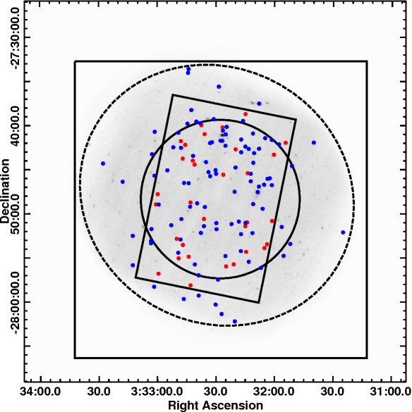
Figure 1: Spatial limits of the different surveys used in this work. The grey-scale image is the combined 2–10 keV 3 Ms image of the XMM-Newton observations, and the regions are the Herschel area (small rectangle), the 4 Ms Chandra area (solid circle), the XMM-Newton area used (dashed circle) and the E-CDFS Chandra area (large square). The radio and Spitzer areas used are all wider than the E-CDFS. The Herschel and the XMM-Newton areas are the boundaries of the “complete” and “broad” samples, respectively (see Sect. 3.3). The sources of the “broad” sample are marked with blue symbols, whereas the sources with FIR flux density upper limits in the “complete” sample are marked with red symbols.

The spatial limits of the different surveys described in this section are shown in Fig. 1. The grey-scale image is the combined 2–10 keV image of XMM-Newton and the regions are the Herschel area limiting the combined GOODS-Herschel–PEP catalogue (small rectangle), the 4 Ms Chandra area (the region where the effective exposure is larger than half of its maximum value; solid circle), the XMM-Newton area (the region where the total integration time is higher than 1 Ms; dashed circle) and the E-CDFS Chandra area (large solid square). The radio and Spitzer areas described above are all wider than the E-CDFS. In this study, we use X-ray sources spanning the entire XMM-Newton region, and use information from all the other surveys to measure their star-formation rates and stellar masses. The smaller Herschel area is used to construct a “complete” sample of X-ray AGNs, where we have FIR detections or upper limits for the majority of the AGNs (see Sect. 3.3), while for the wider area (“broad” sample) we use $\rm 70\,\mu m$ measurements from the FIDEL survey.

3 The sample

In order to avoid high X-ray flux spurious detections due to relatively high background levels, we limit the sample to those sources which have a combined XMM-Newton exposure of 1 Ms or higher in the 2–10 keV band (356 sources in the main and supplementary catalogues of Ranalli et al. in preparation). To better constrain their positions we look for counterparts among the X-ray sources observed with the Chandra surveys, namely in the 2 Ms CDFS catalogue of Luo et al. (2010), the 4 Ms CDFS catalogue of Xue et al. (2011), and the E-CDFS catalogues of Lehmer et al. (2005) and Virani et al. (2006). The characteristic positional uncertainty of Chandra is $\lesssim 1$ arcsec, compared to the 4–5 arcsec of XMM-Newton. We keep Chandra counterparts which are within 5 arcsec of the XMM-Newton position and find 311 unique associations. We also look for counterparts in the $\rm 3.6\,\mu m$ SIMPLE catalogue, using the likelihood ratio method with a matching radius of 5 arcsec, and find another 19 sources with $LR>0.85$ and all with a reliability $>99.9\%$. Most of them lie in the area not covered by the 4 Ms Chandra CDFS survey (see Fig. 1). Our final X-ray catalogue contains 330 sources with good positional constraints ($\lesssim 1$ arcsec) either from Chandra, or from Spitzer-IRAC. Of the 26 sources with no unambiguous Chandra, or Spitzer-IRAC counterpart, 23 are of low-significance ($<5\,\sigma$) and therefore likely spurious, and three are double sources in Chandra, not resolved by XMM-Newton, which we exclude from our sample.

Next, we build the multi-wavelength catalogue of the X-ray sources using all the information available and the likelihood ratio method to select the counterparts, using the positional uncertainties provided in the various catalogues. We first combine the SIMPLE catalogue with both the $K$-selected (Taylor et al., 2009) and the $BVR$-selected (Gawiser et al., 2006) MUSYC catalogues (preferring $K$-selected sources in cases where they are detected in both catalogues) and find the optical-infrared counterparts of the X-ray sources, constraining their positions, and then we look for counterparts in the FIDEL and $\rm 24\,\mu m$-prior Herschel catalogues. We find a counterpart in at least one of the optical or infrared catalogues for 328/330 X-ray sources; one source is too faint to be detected at any other wavelength than X-rays and the other is close to a bright optical-infrared source and is missed by the source detection algorithms. The positions of our optical-infrared counterparts are in good agreement with those of Xue et al. (2011) and Luo et al. (2010) for the sources in common; more than 90% of the counterparts are within 0.7 arcsec of the optical positions given in those catalogues. We use the optical positions to look for radio counterparts in the Kellermann et al. (2008) and Miller et al. (2008), and find 53 matches within a 2 arcsec radius, excluding X-ray sources which have multiple radio counterparts within 10 arcsec, which would be indicative of FR II radio AGNs. For the sub-mm catalogues, because of their large positional uncertainties ($\sim 8$ arcsec) we use the likelihood ratio method to assign a FIDEL-24 counterpart to the sub-mm sources, and if this is the same as the FIDEL-24 counterpart of the X-ray source we consider it as reliable. We find a LABOCA counterpart for five X-ray sources, and an AzTEC for two of these five. Finally, we look for redshifts and find 215 spectroscopic redshift determinations from the various catalogues listed in § 2.6, and 106 photometric redshift estimates. Nine sources have no redshift determination, because they are too faint at optical wavelengths. In the final catalogue we also include FIR upper limits for X-ray sources which are in the area observed by PACS (see Fig. 1) with no detection. There are 155 XMM-Newton sources inside the PACS area and 94 of them are detected. Of the remaining 61, 20 are in regions confused with nearby bright FIR sources, and 41 are upper limits.

3.1 Stellar masses

The most reliable method to derive stellar masses for galaxies is the fitting of their broad-band spectral energy distributions (SEDs) with synthetic stellar templates with known star-formation histories and dust extinction properties (see Shapley et al., 2001; Papovich et al., 2001, for the limitations of the method). The stellar component is important at optical wavelengths $\rm(\lesssim 1\,\mu m)$, but we use the full multi-wavelength information (excluding radio and X-rays) to fit the SEDs. The reason for this is that the AGN can affect the optical properties of the system (see e.g. Pierce et al., 2010), and by fitting a combination of AGN and host templates using the infrared photometric information we can constrain the AGN contribution.

For the optical-infrared SED fitting we use the procedure described in Lusso et al. (2011). We apply a $\chi^{2}$ minimisation method using stellar templates from the Bruzual & Charlot (2003) stellar synthesis code, applying solar metallicity, a mixture of constant and exponentially decaying star-formation rates, and a Galactic disk initial mass function (IMF; Chabrier, 2003). We redden the stellar SEDs using the Calzetti et al. (2000) law, and combine the reddened SEDs with star-formation infrared SEDs from Chary & Elbaz (2001) (105 templates with different FIR profiles in the $\rm 3-1000\,\mu m$ range) and four AGN SEDs from Silva et al. (2004), which span from the optical to the far-infrared with different absorption properties (unabsorbed to $N_{\rm H}\gtrsim 10^{24}\,{\rm cm^{-2}}$). Some characteristic results of the optical-to-infrared SED fitting, as well as a FIR-limit example can be seen in Fig. 2. These are examples of both AGN and starburst dominated SEDs. There is enough optical information (photometry and redshift) to fit an SED for 304 of the 330 sources. Sources with a detection in the Taylor et al. (2009) catalogue (the majority of the optically-detected sources) typically have photometry in nine optical - near-IR bands, and those detected only in the Gawiser et al. (2006) in six bands, which are used for the determination of the stellar masses. We do not take into account upper limits for the fitting, but check that the predicted flux density value of the fitted SED is indeed lower than the limit. The reduced $\chi^{2}$ values of the best-fit models are typically in the 1–10 range, after reprocessing the flux density errors using a quadratic combination with the 10%-level error, to account for the typical flux differences between the SED templates used.

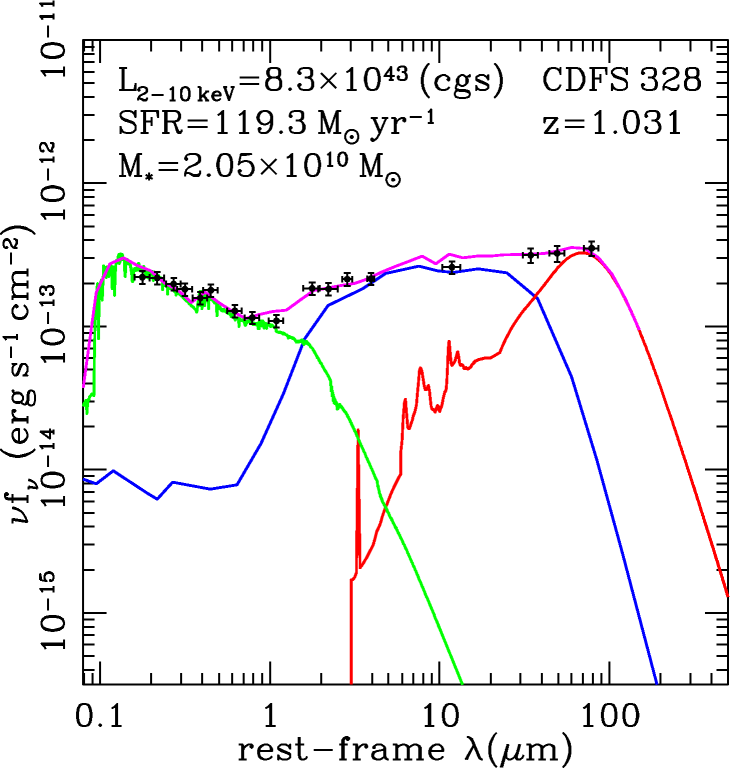
(a)

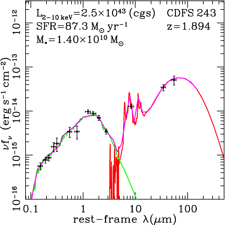
(b)

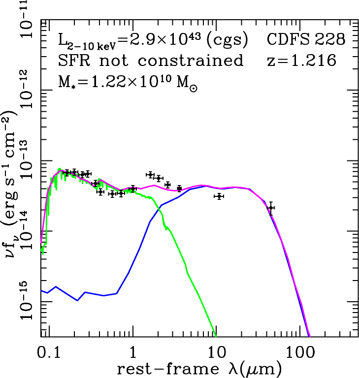
(c)

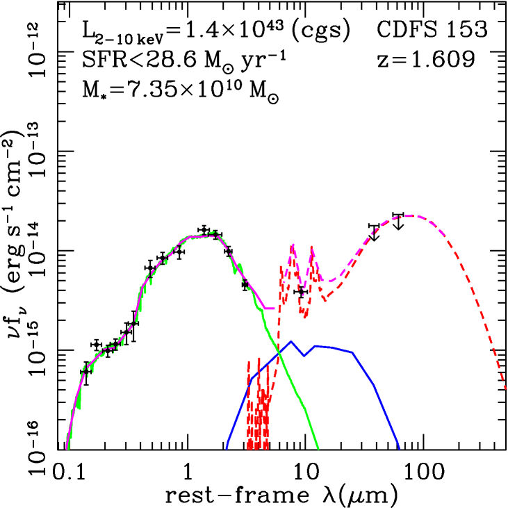
(d)

Figure 2: Examples of the SED fitting used to derive stellar masses and star-formation rates, selected to demonstrate the diversity in the SEDs of the X-ray sample. The star-formation component is plotted in red, the AGN component in blue, and the stellar component in green. In magenta we plot the combination fitted to the data-points. The stellar component is only confined by the optical wavelengths where it usually dominates the flux, but there are cases where we detect a substantial AGN contribution. The star-formation component is confined by the FIR flux with rest-frame wavelength $\rm>20\,\mu m$, and again there are cases where the FIR flux is dominated by the AGN. With downward arrows we plot far-IR upper limits (see Sect. 3.3), where the resulting starburst component is plotted with a dashed line. The numbering in the top-right corners of the panels refers to the preliminary XMM-Newton catalogue number.

The method we use to calculate the stellar masses induces uncertainties both from the choice of the different parameters fitted, and from the $\chi^{2}$ procedure itself. The derived stellar mass values are potentially strongly influenced by such uncertainties, especially at high redshifts, like the majority of the sources in our sample (see also Michałowski et al., 2012). The uncertainties from the parameters included in the stellar synthesis procedure are estimated to be $\sim 0.15$ dex (Bolzonella et al., 2010), and checking the stellar masses and $\chi^{2}$ values of SED fits with different templates and different relative contributions, we estimate the final uncertainty in the stellar masses to be $\sim 0.25$ dex at the 90% confidence level (see Lusso et al., 2012, for a more detailed description of the method). We also note that the use of the Chabrier (2003) IMF causes a slight underestimation of the stellar masses with respect to the Kroupa (2001) IMF, in particular they are on average lower by a factor of $\sim 1.1$ (see Bolzonella et al., 2010; Pozzetti et al., 2010; Hainline et al., 2011). In this work we use the Chabrier (2003) IMF in order to avoid an over-prediction in the number of low-mass stars (Hainline et al., 2011), but we also combine the stellar masses with star-formation rates; the latter are based on infrared luminosities. This star-formation rate proxy uses the Kroupa (2001) IMF for its calibration (see Murphy et al., 2011), so we increase the stellar masses we derive through the SED fitting by a factor of 1.1 to be consistent with the star-formation rates.

3.2 Star-formation rates

Star formation in galaxies affects almost all of their observed properties, from the X-rays to the radio wavelengths, so there are traditionally a number of ways to measure the star-formation rate (SFR). In the cases of AGN hosts we can rule out the X-rays, since they are completely outshone by the AGN (see also § 3.3). In this work we test three methods based only on flux density measurements: i) infrared luminosity, ii) radio luminosity, and iii) optical SED fitting.

3.2.1 Infrared luminosity

The IR luminosity is arguably the most reliable tracer of star-forming activity and is well correlated with other tracers (see Kennicutt, 1998a; Kennicutt & Evans, 2012, for reviews). The IR photons are emitted by the dust surrounding young stars, which is heated by their ultra-violet radiation. In this paper we will use the integrated rest-frame $\rm 8-1000\,\mu m$ luminosity and the equation:

$$\left(\frac{\rm SFR}{\rm M_{\sun}\,yr^{-1}}\right)=3.88\times 10^{-44}\left(\frac{L_{\rm IR}}{\rm erg\,s^{-1}}\right)$$ (1)

from Murphy et al. (2011). In order to measure the IR luminosity we perform the SED decomposition described in § 3.1 anew, using only the infrared data-points from Spitzer and Herschel, the complete Chary & Elbaz (2001) host templates (i.e. including wavelengths $\rm<3\,\mu m$), the AGN templates, and ignoring the synthetic stellar part. The method we use is the same as described in Georgantopoulos et al. (2011a) and Georgantopoulos et al. (2011b), using the SED templates described in § 3.1. We do this in order to avoid the degeneracies in the optical wavelengths between the stellar and AGN light, which could affect the fitted AGN contribution to the infrared luminosity; this way we fit fewer free parameters. For the infrared SED decompositions we require at least three mid-IR points from Spitzer-IRAC to determine the shape of the mid-IR part of the SED, and at least one flux density determination in a rest-frame wavelength higher than $\rm 20\,\mu m$, which we can use to constrain the far-IR part of the SED; there are 125 X-ray sources which comply with these criteria. The FIR flux density determination comes from FIDEL-$\rm 70\,\mu m$ (for $z<2.5$), PACS-$\rm 100\,\mu m$ (for $z<4$), PACS-$\rm 160\,\mu m$, sub-mm (LABOCA and/or AzTEC), or a combination of them. We use the galaxy component (AGN-free) to calculate the star-formation rates, and for 14 cases the AGN component dominates even the longest wavelength IR data-point available, so the determination of the AGN-free part of the IR emission is not reliable. The uncertainties in the IR luminosity values come mostly from the SED decomposition, and a check of the $\chi^{2}$ values of fitting secondary solutions not selected yields an uncertainty of $\sim 0.3$ dex (or a factor of two) in the 90% confidence level, for the vast majority of the sources. The uncertainties arising from the far-IR flux errors are much lower.

3.2.2 Optical SED fitting

The star-formation rate can be derived as a by-product of the optical SED fitting performed in § 3.1, using the star-formation history and age assumed, and the normalisation from the photometry. Similar methods have been widely used in deep fields, including the CDFS (e.g. Brusa et al., 2009), especially if far-infrared photometry is not available. In the next paragraph we will test its reliability, since it is a highly model-dependent method with systematic uncertainties arising mainly from the IMF, star-formation history and extinction law used (see Bolzonella et al., 2010).

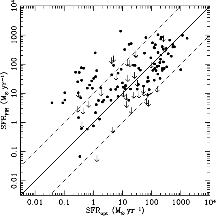
(a) FIR - optical SED

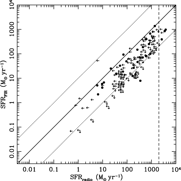
(b) FIR - radio

Figure 3: Comparison of the star formation rates of X-ray sources, measured using the infrared $\rm 8-1000\,\mu m$ luminosity, and the optical SED fitting (a), or the 1.4 GHz radio luminosity (b). Black circles mark reliable fits in both optical and far-infrared (or radio) wavelengths, excluding cases where the AGN SED dominates even the longest wavelength flux density available. Sources spanning over the whole 3 Ms XMM-Newton region are used in these plots, while the downward arrows refer to Herschel non-detections in the PACS area (35 cases), and leftward arrows in the right panel refer to radio upper limits spanning over the whole XMM-Newton region (112 cases). The solid and dashed lines in both panels represent the 1:1 relation and the $\rm\pm 1\,dex$ deviation, respectively, and the vertical dashed line in the right panel marks the calculated star-formation rate of a source having $L_{\rm 1.4\,GHz}=10^{24.5}\,{\rm W\,Hz^{-1}}=10^{31.5}\,{\rm erg\,s^{-1}\,Hz^{-1}}$. The significant deviation form the 1:1 relation of both cases and the significant scatter of the optical SED (left) case prevent us from using any of the two SFR tracers in this paper.

In Fig. 3a we plot the star-formation rate measured from the infrared luminosity of the sources detected in the far-infrared against the SFR measured from the optical SED fitting after correcting for extinction, excluding the AGN contribution for both cases. All X-ray sources with an infrared measurement with rest-frame wavelength above $\rm 20\,\mu m$ and an optical identification (in MUSYC) are plotted with a circle. We exclude these 14 cases where, according to the SED decomposition, the flux density of the longest wavelength data-point is dominated by the AGN, so that the SFR cannot be constrained (see Fig. 2c). In Fig. 3a we also include SFR upper limits for the X-ray sources in the Herschel area which are not detected by Herschel; for one of the 41 X-ray sources with FIR upper limits we do not have any photometric data-points to perform an SED fitting in the mid-infrared, while another four are not detected in the optical, or have no redshift determination, so 36 upper limits are plotted in Fig. 3a. The solid line is the 1:1 line and the dotted lines mark the $\pm 1$ dex region. We can see that out of the 109 points of Fig. 3a, 79 are between the dotted lines, while for 29 sources using the optical SEDs underestimates the SFR by more than an order of magnitude; for one (and two upper limits) the SFR is overestimated by more than an order of magnitude, assuming that the infrared SFR is reliable. The star-formation rate estimated from the optical SED is a highly model-dependent value, and is very sensitive to the star-formation history assumed in the stellar synthesis models, which shape the optical SED. It is also sensitive to dust extinction, which would cause an underestimation of the SFR, explaining the behaviour we see in Fig. 3a. Due to this large scatter and systematic offset, we do not rely on the optical SED fitting to derive star-formation rates and use it only for stellar mass determinations. The stellar mass is an integrated value and therefore less sensitive to the assumed star-formation history. Moreover, we do not detect any obvious dependence of the difference between the SFR determination using the two estimators on X-ray or optical classes, which would indicate AGN contamination as the cause of the scatter.

3.2.3 Radio luminosity

The radio luminosity of star-forming galaxies is tightly correlated with their infrared luminosity (see Condon, 1992, for a review), and this correlation holds even for cosmologically significant redshifts ($z\approx 2$; Appleton et al., 2004; Ivison et al., 2010); we test it in this work as a possibility to derive the star-formation rates in X-ray sources without far-infrared detections. The radio emission in star-forming systems is generated by synchrotron radiation from relativistic electrons accelerated by supernova induced shocks and free-free emission in H ii regions. The caveat is that AGNs themselves can produce radio emission through radio jets or compact high surface-brightness synchrotron core emission from relativistic electrons heated by the AGN. There is a dichotomy in the radio power of quasars (Miller et al., 1990), with sources having $L_{\rm 5\,GHz}\gtrsim 10^{25}\,{\rm W\,Hz^{-1}}$ being characterised as “radio-loud” and their power source being closely connected to the AGN, and sources having $L_{\rm 5\,GHz}\lesssim 10^{25}\,{\rm W\,Hz^{-1}}$ being characterised as “radio-quiet” and having a controversy about their power source. Alternatively, the radio to optical flux ratio is used in some studies to differentiate between radio-quiet and radio-loud AGNs (Kellermann et al., 1989). However, the dichotomy between radio-loud and radio-quiet sources is not clear if more complete samples are used (e.g. White et al., 2000), with many objects in the “intermediate” region, making the transition smooth with only a vague limit. Recently, Padovani et al. (2011), using the luminosity functions of different types of radio sources in the CDFS, argue that the major contribution to radio power in the diffuse part of radio-quiet AGNs comes from star-formation, though taking a somewhat stringent limit to characterise the radio sources based on their radio luminosities ($L_{\rm 1.4\,GHz}=10^{24.5}\,{\rm W\,Hz^{-1}}=10^{31.5}\,{\rm erg\,s^{-1}\,Hz^{-1}}$, combined with other observational characteristics).

For this work we test how reliable the radio luminosities are in estimating star-formation rates for an AGN sample using the VLA 1.4 GHz flux densities from Kellermann et al. (2008) and Miller et al. (2008), also checking the VLBI catalogue of Middelberg et al. (2011) to exclude any high surface-brightness compact cores, characteristic of non-thermal nuclear emission, not connected to the star formation (e.g. Giroletti & Panessa, 2009). We calculate the radio luminosities using

$$L_{\rm 1.4\,GHz}=4\pi d_{\rm l}^{2}S_{\rm 1.4\,GHz}(1+z)^{\alpha-1}$$ (2)

where $\alpha$ is the radio spectral index, assuming $S_{\nu}\propto\nu^{-\alpha}$, and it is calculated from the relative radio flux densities at 1.4 and 5 GHz. In cases where the 5 GHz flux density is not available we assume $\alpha=0.8$, characteristic of synchrotron emission (see Condon, 1992). There are 53 X-ray sources with a radio counterpart within 2 arcsec and without another radio source closer than 10 arcsec, the latter would suggest an FR II radio-loud source. Eight of these sources have a high surface-brightness core detected with VLBI with a flux density above 0.5 mJy, and are removed from the test sample, and a further eight are radio-loud according to the $L_{\rm 1.4\,GHz}>10^{31.5}\,{\rm erg\,s^{-1}\,Hz^{-1}}$ criterion (three are also detected in the far-infrared and are included in Fig. 3b). The star-formation rate is calculated using

$$\left(\frac{\rm SFR}{M_{\sun}\,{\rm yr}^{-1}}\right)=6.35\times 10^{-29}\left(\frac{L_{\rm 1.4\,GHz}}{\rm erg\,s^{-1}\,Hz^{-1}}\right)$$ (3)

(Murphy et al., 2011). In Fig. 3b we plot the star-formation rates from the infrared and radio luminosities for sources being detected in both bands, keeping the same range and symbols as in Fig. 3a. We also plot the radio and infrared (for the Herschel area) upper limits with arrows. The scatter in this case is significantly lower than in Fig. 3a. However, the mean $\rm\log(SFR_{IR}/SFR_{1.4\,GHz})$ of the radio detections is $-0.48$ (without taking into account the VLBI sources and the upper limits) with a standard deviation of $\sigma=0.39$. The dashed vertical line in Fig. 3b marks the calculated SFR of a source having $L_{\rm 1.4\,GHz}=10^{31.5}\,{\rm erg\,s^{-1}\,Hz^{-1}}$, thus being border-line radio-loud according to the limit of Padovani et al. (2011). If we keep this limit and calculate the mean $\rm\log(SFR_{IR}/SFR_{1.4\,GHz})$ of only the radio-quite objects, its mean and standard deviation become $-0.45\pm 0.40$, so there is still contamination from the AGN emission; most probably we are detecting in the radio band those sources which are in the top of the radio flux distribution, something which is supported by the location of the upper limits. Because of this contamination, we do not use the radio power as a star-formation proxy in our AGN sample.

3.3 Final sample

We start with a sample of 356 X-ray 2–10 keV selected sources from the 3 Ms XMM-Newton survey with a total integration time more than 1 Ms, 330 of which have good ($\lesssim 1$ arcsec) positional constraints from Chandra or Spitzer. We have enough optical information to fit an SED and calculate the stellar masses for 304 of these 330 sources. On the other hand, we rely on the infrared flux density to constrain the SFR of our sample, and there are 111 sources with an SFR measurement from the FIR flux. For 109 of them we can also calculate the stellar mass from the optical SED.

As we are dealing with faint X-ray fluxes, there is the possibility that for some of the X-ray sources the X-rays trace normal star-forming galaxies instead of the AGNs (Ranalli et al., 2003; Bauer et al., 2004). In Fig. 4 we plot the hard X-ray flux densities against their optical ($R$-band) magnitudes. The lines mark the $-1<\log(f_{\rm x}/f_{\rm opt})<1$ region where the bulk of the AGNs are expected (see e.g. Stocke et al., 1991; Elvis et al., 1994; Xue et al., 2011). Sources with $\log(f_{\rm x}/f_{\rm opt})<-1$ are candidates for being normal galaxies instead of AGNs (see Tzanavaris et al., 2006; Georgakakis et al., 2006). Moreover, most normal galaxies have X-ray luminosities not exceeding $\rm 10^{42}\,erg\,s^{-1}$, except for a few extremely star-forming sources, mainly detected in sub-mm wavelengths (see e.g. Alexander et al., 2005; Laird et al., 2010). Sources with luminosities below the $\rm 10^{42}\,erg\,s^{-1}$ limit are plotted with open circles in Fig. 4. There are 10 sources compliant with both the $f_{\rm x}/f_{\rm opt}$ and the $L_{\rm x}$ criteria, and they do not show any signs of obscuration in their X-ray spectra, so we remove them from the AGN sample.

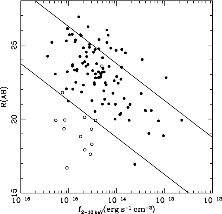
Figure 4: Optical magnitude against 2–10 keV flux density for the XMM-Newton sources with robust SFR estimations. The lines mark the $-1<\log(f_{\rm x}/f_{\rm opt})<1$ region and open symbols sources with $L_{\rm x}<10^{42}\,{\rm erg\,s^{-1}}$. We exclude the 10 sources which have both $L_{\rm x}<10^{42}\,{\rm erg\,s^{-1}}$ and $\log(f_{\rm x}/f_{\rm opt})<-1$ from our final sample, as normal galaxy candidates.

A fundamental property of each galaxy is its specific star-formation rate (sSFR), which is defined as the ratio of its star-formation rate to its stellar mass. It is indicative of how efficient the galaxy is forming stars. To calculate the sSFR for the AGNs in our sample, we use the star-formation rates measured from the infrared luminosity. We have calculated the sSFR for 99 X-ray AGNs, 77 with spectroscopic redshift and 22 with photometric redshift. The SFR, stellar mass, sSFR and redshift histograms are shown in Fig. 5.

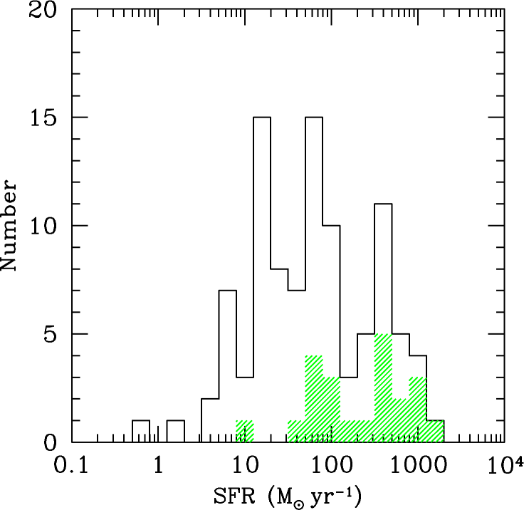
(a)

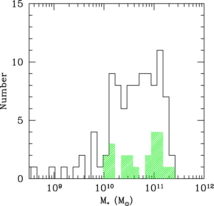
(b)

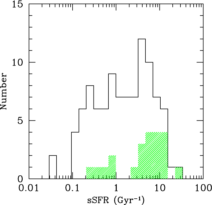
(c)

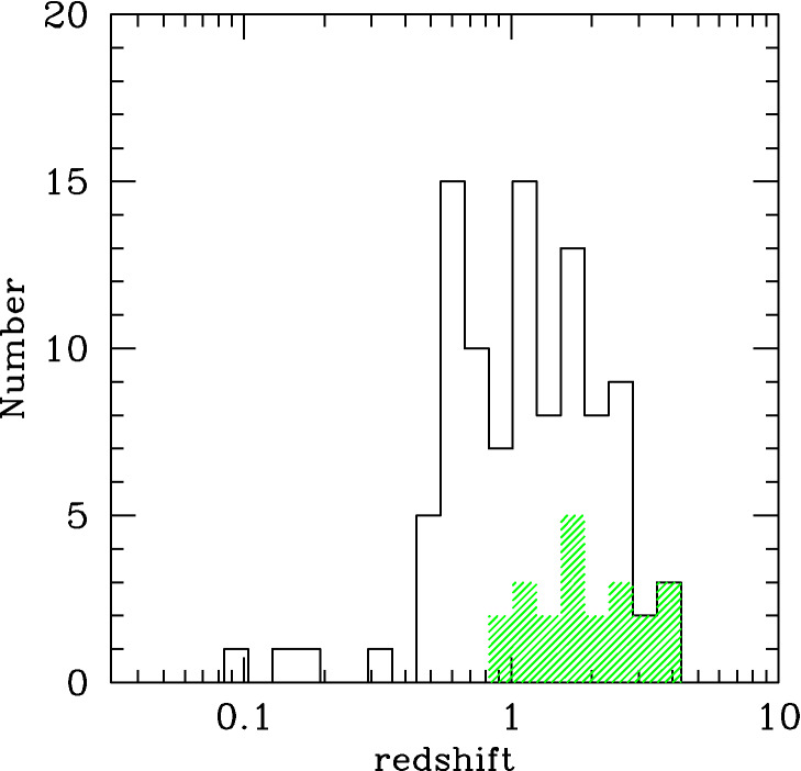
(d)

Figure 5: Histograms of the basic properties (star-formation rates, stellar masses, specific star-formation rates, and redshifts) for the 99 hosts of the X-ray AGN sample used in this work. The shaded histograms show the same properties for X-ray QSOs, i.e. sources with $L_{\rm x}>10^{44}{\rm\,erg\,s^{-1}}$.

The sample described in the previous paragraph (hereafter the “broad” sample) is not a complete sample of X-ray detected AGNs, because of the various selections of the sources, which limit their number from 356 to 99. This incompleteness might affect the statistical properties. In order to account for that, we create a more complete sub-sample constrained in the Herschel area where we have the most sensitive far-IR measurements. In this area (marked with the small rectangle in Fig. 1) for the X-ray sources for which a far-IR counterpart is not found, a FIR upper limit is calculated from the sensitivity map of the GOODS-Herschel–PEP survey. Thus, we have 155 X-ray sources, 94 of them are detected in the FIR, and for 41 we can calculate an upper limit to their $\rm 100\,\mu m$ and $\rm 160\,\mu m$ fluxes. Twenty sources lie within a 10 arcsec region of a nearby bright FIR source and an upper limit cannot be calculated, they are however a random sub-sample, not affecting the completeness. Out of the 135 (155-20) sources, eight are associated with normal galaxies not hosting an AGN, a further 12 do not have sufficient optical or mid-infrared information, or a redshift estimate for an SED fit, and for a further seven the emission from the AGN dominates over the FIR flux (the AGN-related flux go the highest wavelength data-point is higher than the star-formation related), making a star-formation measurement not reliable. Summing up, we calculated the SFRs and stellar masses of 108 out of the 127 ($\approx 85\%$) X-ray AGNs in the GOODS-Herschel region, for which a FIR flux determination is possible (76 detections and 32 upper limits). Hereafter we will call this the “complete” sample. The basic properties (2–10 keV luminosities and redshifts) of the complete sample are shown in Fig. 6 with red symbols (filled and open circles for FIR detections and limits, respectively), while the properties of the overall sample are plotted in black symbols, and the rest of the X-ray sources are plotted in grey crosses.

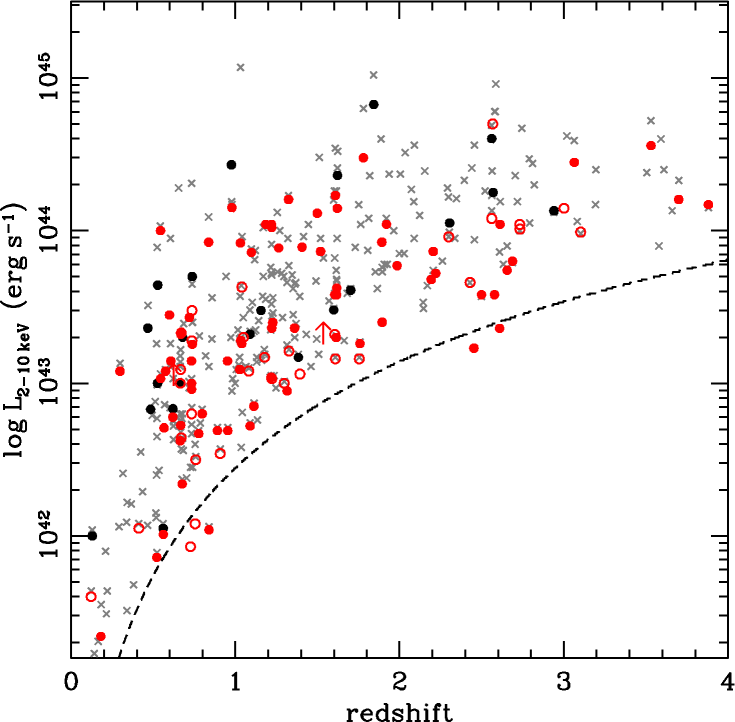
Figure 6: 2–10 keV luminosities against redshift for all the X-ray sources with redshift determinations in the 3 Ms XMM-Newton survey. The original parent sample is plotted in grey crosses, while black and red filled circles are plotted for the X-ray AGNs with both a stellar mass and a SFR measurement (“broad” sample). Red symbols represent sources in the GOODS-Herschel-PEP area, filled for Herschel detections and open for FIR upper limits (“complete” sample). The line is the $\rm 6.5\times 10^{-16}\,erg\,s^{-1}\,cm^{-2}$ flux limit, assuming $\Gamma=1.7$.

4 Results

4.1 sSFR-$L_{\rm x}$

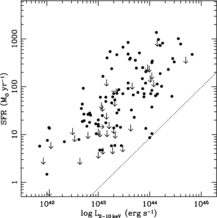
Figure 7: Star-formation rate against hard X-ray luminosity for X-ray selected AGNs. We plot values of 99 far-infrared detected X-ray AGNs, and 32 FIR upper limits in the area covered by the deep Herschel survey. The dotted line is the expected FIR luminosity of a pure-AGN source, translated into SFR (see Mullaney et al., 2011). We find a strong correlation between the star-formation rate and the X-ray luminosity.

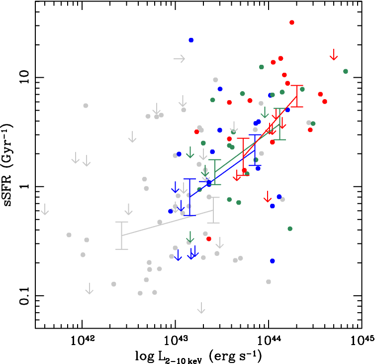
Figure 8: Specific star-formation rate against hard X-ray luminosity for X-ray selected AGNs. The grey, blue, green and red symbols refer to $z<1.120$, $1.120<z<1.615$, $1.615<z<2.455$ and $z>2.455$, respectively. The error-bars and their associated lines refer to the mean luminosities and specific SFRs of the high- and low-luminosity bins within each redshift bin, using the Kaplan-Meier estimator (see Sect. 4.1). We do not detect a significant correlation between the X-ray luminosity and sSFR for the lowest redshift bin, but do detect a significant correlation for higher redshifts ($z\gtrsim 1$).

In previous studies there has been a controversy about the existence of an observational connection between the AGN and the host galaxy activity. In Fig. 7 we plot the SFR against the hard X-ray luminosity of the 99 X-ray AGNs with an estimate of the SFR described in the previous section and the 32 upper limits. There are also two X-ray sources with lower limits in their X-ray luminosities. These are Compton-thick sources whose X-ray spectra are dominated by a reflection component according to the spectral fits, and their unobscured luminosities cannot be determined. The lower limits in Fig 8 are their observed luminosities. Because of the limits, for the statistical analysis we use the ASURV package (Rev. 1.3 LaValley et al., 1992), which implements the methods presented in Feigelson & Nelson (1985) and Isobe et al. (1986). Using the generalised Kendall’s $\tau$ method in order to include upper limits, and all the data-points of Fig. 7, we find that the SFR is strongly correlated with the hard X-ray luminosity, with a null hypothesis probability lower than 0.01%. To simulate a mass-matched sample and study the activity of the host independent of its size, we calculate the specific SFRs of the sample and plot it against the X-ray luminosity in Figure 8. Performing the same method, we find again that the two values are strongly correlated. However, Mullaney et al. (2012a) have shown that the correlation between the X-ray and the infrared luminosity is sensitive on the evolution of the infrared luminosity with redshift, and this might be affecting the sSFR-$L_{\rm x}$ correlation we observe here. To test this hypothesis we apply the partial correlation test of Akritas & Siebert (1996) and find significant correlations of the sSFR with both redshift and X-ray luminosities at the $4.6\sigma$ and $4.4\sigma$ levels, respectively. However, this partial correlation test tends to incorrectly reject the null-hypothesis in cases where the two “independent” parameters (here $L_{\rm x}$ and $z$) are also correlated with each other (see Kelly et al., 2007) as in this case, which limits the reliability of the test.

In order to further check the effect of the redshift in the sSFR-$L_{\rm x}$ correlation, we divide our sample into six redshift bins, containing a roughly equal number of data-points (21 or 22), and repeat the Kendall’s $\tau$ method for each bin separately and for different combinations. The description of the redshift bins and the results of the test (null hypothesis probability) are shown in Table 1. We can see that there is no correlation at lower redshifts, but there is a possible correlation for $z>1.15$ (bins 4, 5, 6) with $\gtrsim 95\%$ significance. If we merge adjacent bins in order to increase the number of data-points in each bin, the correlation is again found for $z>1.12$ (bins 4-5, 5-6) with $>99.8\%$ significance. In this case however the redshift dependence is not negligible. We also note that within the redshift bins the sample is almost luminosity-limited. To further check if the X-ray flux limit affects the previous result, we exclude sources with X-ray luminosities lower then the luminosity limit of the highest redshift limit of each redshift bin, to create truly luminosity-limited sub-samples. Repeating the analysis in those sub-samples, the previous result does not change significantly, except in the highest-redshift bin ($z>2.305$). In Fig. 8 we colour-code the data-points with respect to their redshifts, in grey we plot bins 1-2-3, in blue bin 4, in green bin 5 and in red bins 6; the results of this binning are shown in the last column of Table 1. We divide each data compilation into a low-luminosity and a high-luminosity bin including an equal number of sources, and plot the mean sSFR and its associated error, calculated using the Kaplan-Meier estimator in ASURV, and the mean luminosity of the bin. The sSFR-$L_{\rm x}$ correlation is evident for the blue, green and red data-points ($z>1.15$).

A possibly important factor affecting the previous analysis is the FIR selection of the sources of our final “broad” sample, which reduces the number of X-ray sources from 356 to 99, being biased in favour of sources with higher SFRs. In order to check whether this has an effect on the apparent sSFR-$L_{\rm x}$ correlation, we repeat the previous analysis in the small area covered by the GOODS-Herschel survey (the “complete sample”; see Figs. 1 and 6). In this case, the analysis is performed in broader redshift bins due to the smaller number of sources, and the results are similar to those described in the previous paragraph; there is no sign of a sSFR-$L_{\rm x}$ correlation below $z\lesssim 1.2$, but above this redshift the correlation is $>95\%$ significant.

We note here that there is a small number of X-ray sources, which are detected in the far-infrared in a rest-frame wavelength $\rm\lambda>20\,\mu m$, but its flux density is dominated by the AGN emission, according to the SED decomposition performed. There are 14 such cases in the “broad” sample and seven in the “complete” sample with redshifts $z\sim 1-3$. These sources could populate the low-(s)SFR - high-$L_{\rm x}$ area, however their far-IR luminosities cannot be constrained, not even with an upper limit. If we consider the SFR estimations from the optical SEDs, although unreliable, they are consistent with the (s)SFR-$L_{\rm x}$ correlation. Moreover, their number is $\sim 10\%$ of the sample used, so we are confident that they will not affect the result.

Table 1: Results of Kendall’s $\tau$ method for the correlation between the specific star-formation rate and the hard X-ray luminosity for different redshift bins. The null hypothesis probability in each redshift bin is shown in column 3 and in combinations of bins in columns 4 and 5, with a lower null hypothesis probability meaning a tighter correlation.

Bin	number of sources	redshift range	Null Hypothesis (%)	Null Hypothesis (%)	Null Hypothesis (%)
1	21	$0.000-0.620$	34	7.9 (bins 1–2)	1.5 (bins 1–3)
2	22	$0.625-0.755$	8.5	4.3 (bins 2–3)
3	22	$0.759-1.113$	43	9.5 (bins 3–4)
4	22	$1.156-1.599$	5.4	0.18 (bins 4–5)	5.4 (bin 4)
5	22	$1.605-2.299$	0.97	0.11 (bins 5–6)	0.97 (bin5)
6	22	$>2.305$	5.2		5.2 (bin 6)

4.2 Redshift evolution

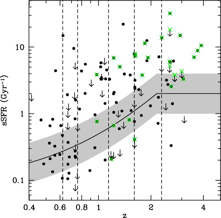
(a) specific SFR

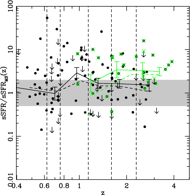
(b) “starburstiness”

Figure 9: Evolution of the specific SFR and the “starburstiness” with redshift for X-ray selected AGNs with long wavelength information. The dashed vertical lines refer to the redshift bins of Table 1, the solid line in panel (a) is the expected main sequence sSFR according to Equation 4, and the grey areas denote the limits of the starburst and quiescent areas. Their borders are double and half the main-sequence sSFR, according to Elbaz et al. (2011). Green crosses mark the positions of X-ray QSOs having intrinsic $L_{\rm 2-10\,keV}>10^{44}\,{\rm erg\,s^{-1}}$. In panel (b), the solid lines and respective data-points are the running means of the “starburstiness” for X-ray AGNs and QSOs in the “broad” AGN sample, and the dashed lines are the running means of the “complete” X-ray AGN sample (see Sect. 3.3). There is a general trend for the sSFR of AGN hosts to follow the main sequence, so that the median “starburstiness” is constant with redshift. The QSO hosts on the other hand have sSFRs which are somewhat higher.

The average sSFR of star-forming galaxies increases with redshift at least up to $z\approx 2$ (Elbaz et al., 2007; Daddi et al., 2007), and in this section we investigate how the hosts of an AGN evolve with respect to the general population. In Fig. 9a we plot the sSFR of the AGN hosts against the redshift. The vertical lines refer to the redshift bins of Table 1, while the solid curve is the expected main-sequence sSFR, according to

$${\rm sSFR_{MS}}[{\rm Gyr^{-1}}]=\left\{\begin{array}[]{l l}26\times t^{-2.2}_{\rm cosmic},&z<2.156\\ 2,&\rm otherwise\end{array}\right.$$ (4)

where $t_{\rm cosmic}$ is given in Gyr. The grey area denotes the borders of the starburst and quiescent areas, defined as double and half the main sequence sSFR, respectively (Elbaz et al., 2011). We note here that the increase of the main-sequence sSFR does not continue forever, and in Elbaz et al. (2011) the density of data-points supporting the above relation dramatically decreases at $z\gtrsim 2.5$. There is evidence that the main-sequence sSFR is constant above $z\approx 2$ (Stark et al., 2009; González et al., 2010) with a value of $\rm sSFR_{MS}\approx 2\,Gyr^{-1}$. According to the above relation the value of $\rm sSFR_{MS}=2$ is reached at $z=2.156$, so above this redshift we assume a constant relation. There is a hint that the hosts of the AGNs in our sample are mostly in the main-sequence and starburst regions, while they generally follow the behaviour of the main sequence with redshift. With green crosses we mark the positions of X-ray QSOs having intrinsic $L_{\rm 2-10\,keV}>10^{44}\,{\rm erg\,s^{-1}}$. The majority of them (19/25 sources) are consistent with being in the starburst region with ${\rm sSFR/sSFR_{MS}}(z)>2$.

This behaviour is also evident if we plot the “starburstiness” against redshift in Fig. 9b. The “starburstiness” is the ratio of the sSFR of the source over the main-sequence value at the given redshift. The vertical dashed lines in Fig. 9b are identical to those in Fig. 9a, and the grey area again marks the main sequence. The symbols of the data-points are identical to Fig. 9a (black for all the sources and green for X-ray QSOs). In each redshift bin we also show the average “starburstiness” and its associated statistical uncertainty calculated using the Kaplan-Meier estimator. For the QSO case we have re-binned the data into four redshift bins to improve the statistics of the sample. The behaviour seems to depend on redshift: the QSOs in the first redshift bin with $0.976\leq z\leq 1.499$ have an average sSFR consistent with that of the overall population, while higher redshift QSOs are on average more “starbursty”, having sSFR more than double that of the main sequence.

To check how much the complex source selection affects those results, we repeat the previous analysis for the “complete” sample, where we have FIR upper limits for most of the X-ray sources. We use the same technique, and the result is shown with the dashed lines in Fig. 9b. It is consistent within the statistical uncertainty with that of the “broad”sample. For the QSO case however, the difference between the complete and the broad sample is significant in the first redshift bin, owing to the scarcity of such objects. The mean sSFR of the QSOs seems to be in the main sequence for $z\lesssim 2$ and in the starburst region for higher redshifts.

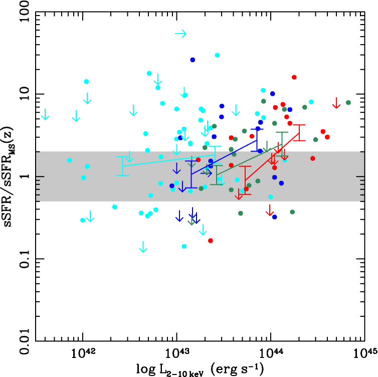
Figure 10: “Starburstiness” against (2–10) keV X-ray luminosity for the sources in our sample. The grey area is the same as in Fig. 9 and the data-points and error-bars are as in Fig. 8, substituting the gray point with cyan. We again do not detect any significant correlation between the “starburstiness” and the X-ray luminosity for $z\lesssim 1$, but there is a correlation for $z\gtrsim 1$, within the redshift bins.

In order to further investigate how the “redshift effect” affects the correlation found between the sSFR and the hard X-ray luminosity, in Sect. 4.1 we plot the starburstiness defined in this section against the X-ray luminosity in Fig. 10. The results of the statistical analysis (null hypothesis probability) of the same redshift bins as in Table 1 are presented in Table 2. The analysis shows again a $\gtrsim 95\%$ correlation for redshifts $z\gtrsim 1$ and no correlation at lower redshifts. We therefore assume that the correlation between the host and galaxy activity is not affected by the evolution of the infrared luminosity with redshift.

Table 2: Results of Kendall’s $\tau$ method for the correlation between the starburstiness and the hard X-ray luminosity for different redshift bins. The null hypothesis probability in each redshift bin is shown in column 3 and in combinations of bins in columns 4 and 5.

Bin	number of sources	redshift range	Null Hypothesis (%)	Null Hypothesis (%)	Null Hypothesis (%)
1	21	$0.000-0.620$	84	31 (bins 1–2)	4.4 (bins 1–3)
2	22	$0.625-0.755$	6.7	4.5 (bins 2–3)
3	22	$0.759-1.113$	69	29 (bins 3–4)
4	22	$1.156-1.599$	6.0	0.5 (bins 4–5)	6.0 (bin 4)
5	22	$1.605-2.999$	1.0	3.7 (bins 5–6)	1.0 (bin 5)
6	22	$>2.305$	5.2		5.2 (bin 6)

4.3 sSFR-$N_{\rm H}$

In earlier studies there have been some hints of a correlation between the star-forming activity of the host and the AGN obscuration in the X-rays. Page et al. (2004) found that X-ray absorbed sources are more likely to be detected at sub-mm wavelengths because of their extreme star-formation rates, although the absorbed AGN sample consisted only of type I (broad-line) QSOs (Page et al., 2001), which are not a representative sample. Moreover, Alexander et al. (2005) found that the majority of radio-detected SCUBA sub-mm sources are consistent with being heavily obscured AGNs, with $N_{\rm H}\gtrsim 10^{23}\,{\rm cm^{-2}}$, although the active nucleus is not bolometrically dominant. Bauer et al. (2002) found hints that X-ray sources with sub-mJy radio counterparts (tracing star formation) are, on average, more obscured than the unmatched population, confirmed by Georgakakis et al. (2004). Subsequently, Rovilos et al. (2007) using a combination of the 1 Ms CDFS and the E-CDFS surveys found that such a trend was confined only to AGNs with any evidence for X-ray obscuration ($N_{\rm H}>10^{21}\,{\rm cm}^{-2}$), linking it with line-of-sight effects. However, deeper surveys both in X-rays and at infrared wavelengths failed to reproduce those results (e.g. Lutz et al., 2010; Rosario et al., 2012; Trichas et al., 2012). Here, we use the deepest XMM-Newton survey, providing good quality X-ray spectra, combined with the deepest Herschel PACS observations, and an SED decomposition technique to clarify this issue. In Fig. 11a we plot the hydrogen column density of the sources for which we have good X-ray spectra against their star-formation rates. We apply a value of $N_{\rm H}=10^{20}\,{\rm cm}^{-2}$ to sources which show no signs of obscuration and $N_{\rm H}=5\times 10^{24}\,{\rm cm}^{-2}$ to Compton-thick AGNs. We do not find any significant correlation between the two values. Using the Kendall’s $\tau$ method we find a null-hypothesis probability of 90%. Excluding unobscured AGNs or splitting the data into redshift bins does not change this result; the null hypothesis probability is always higher than 20%. Neither is there a significant correlation in the high luminosity AGN ($L_{\rm x}>10^{44}{\rm\,erg\,s^{-1}}$) or the high redshift ($z>1.5$) sub-samples. In order to simulate a mass-matched sample and correct for any redshift effects in the column density and sSFR values (e.g. Hasinger, 2008) we also plot the specific SFR and the starburstiness against $N_{\rm H}$ in Figs. 11b and 11c. Performing all the previous tests, we again do not find any significant correlation, except for the sSFR and starburstiness of AGNs with $0.7<z<1.4$, where we find hints of an anti-correlation at the 95% level. However, considering the behaviour of the overall sample and the complex selection effects to shape that sub-sample, we do not consider it important. This behaviour is in broad agreement with models assuming a clumpy absorber (Elitzur & Shlosman, 2006; Nenkova et al., 2008), where the absorption strongly depends on the number of absorbing clumps crossing the line-of-sight, however there is a number of obscured AGNs (with $N_{\rm H}>10^{22.5}\,{\rm cm}^{-2}$) and ${\rm sSFR/sSFR_{MS}}(z)<1$ which are still hard to explain with these models.

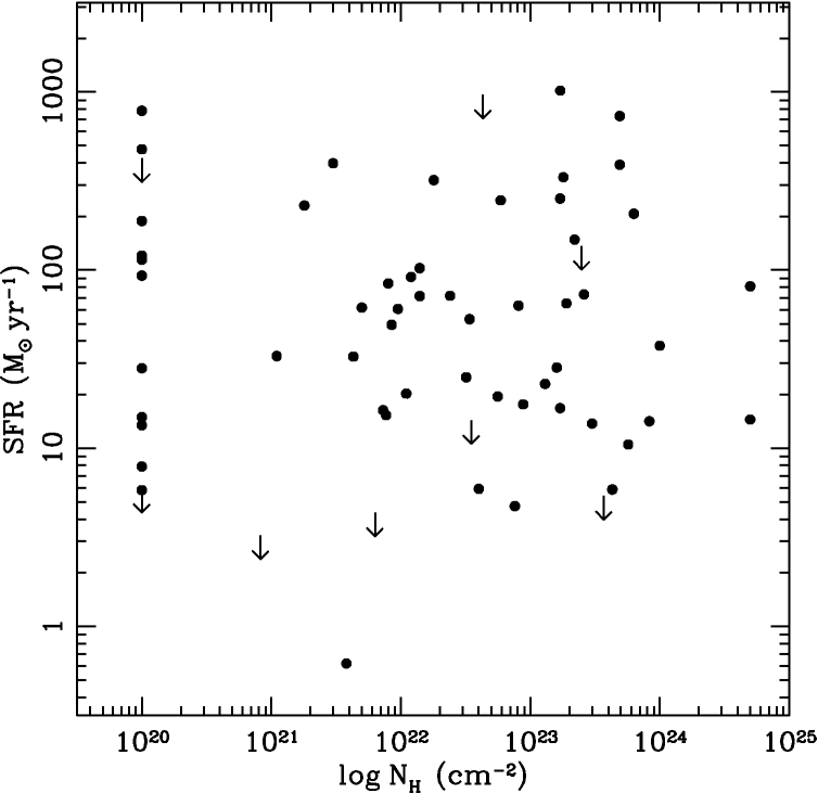
(a) SFR

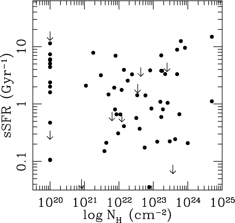
(b) specific SFR

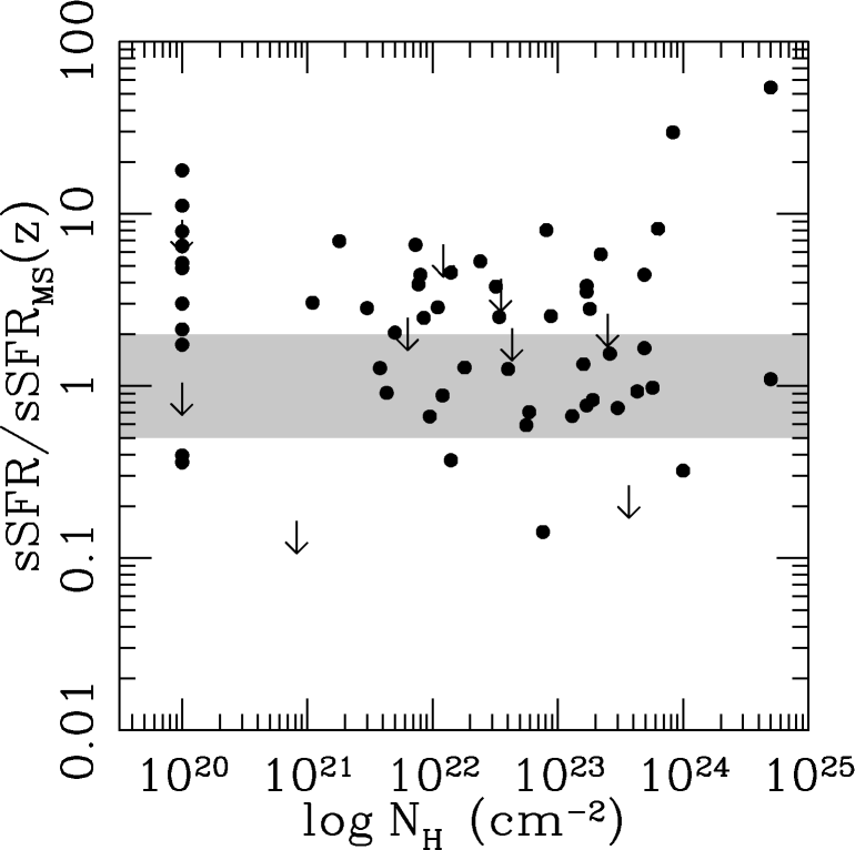
(c) “starburstiness”

Figure 11: Star-formation rate, specific star-formation rate, and “starburstiness” plotted against the hydrogen column density for 65 sources with XMM-Newton spectra and robust SED fitting (including nine with Herschel upper limits). The grey area in panel (c) is the main-sequence, as in Figs. 9 and 10. The errors on the hydrogen column density are in the range of $\lesssim 10\%$ to 30%. We do not detect any significant correlation between the two values, even if we split the sample into redshift or luminosity bins, in any of the three plots.

4.4 Rest-frame colours

The colour-magnitude diagram (CMD; the rest-frame $U-B$ or $U-V$ colour plotted against the absolute $B$ or $V$ magnitude) is used in a number of studies to check the evolutionary stage of the AGN hosts. The hosts of AGNs are concentrated in and around the “green valley” (Nandra et al., 2007; Rovilos & Georgantopoulos, 2007; Silverman et al., 2008; Georgakakis et al., 2008; Hickox et al., 2009; Georgakakis & Nandra, 2011), which is thought to signpost the transition phase from a starburst to a “dead” elliptical. There are however a number of factors that affect the position of a source (especially an AGN) in the CMD making the meaning of the above observation unclear. For example, it has been noted that both the AGN contribution and dust obscuration can alter the observed optical colours of the AGN hosts (Pierce et al., 2010; Cardamone et al., 2010b; Lusso et al., 2011), making them bluer or redder. Moreover, AGNs are usually found in relatively high stellar mass hosts ($M_{\star}\approx 10^{10}-10^{12}\,{\rm M_{\sun}}$; Kauffmann et al., 2003; Brusa et al., 2009; Xue et al., 2010; Mullaney et al., 2012a, this study), and that in turn makes them “avoid” the blue cloud; it is observed that the concentration of AGNs around the “green valley” is not detected when using mass-matched samples (Silverman et al., 2009; Xue et al., 2010; Mullaney et al., 2012a). In this section we use the sample of AGNs for which we have an independent way to measure the star-formation activity, to check the validity of the colour-magnitude diagram without correcting the optical magnitudes for the host contribution or dust reddening. In addition, we use a colour-mass diagram instead of the colour-magnitude approach, in order to simulate a mass-matched sample.

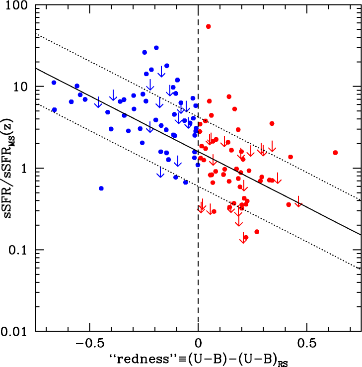
Figure 12: Starburstiness against deviation from the dividing line between red and blue galaxies for the sources of our sample. With blue and red symbols are plotted galaxies in the blue cloud and the green valley, and red-sequence galaxies respectively; the dividing line (the border of the red sequence) is the dashed vertical line, calculated from the parametrisation of Peng et al. (2010). The lines denote the best-fit model and its standard deviation, according to Equation 5.

The positions of the red sequence, blue cloud and green valley in the colour-magnitude (and colour-mass) diagram are strongly dependent on redshift (Bell, 2003; Borch et al., 2006; Peng et al., 2010). In this section we use the $U-B$ rest-frame colours of a sample of AGN hosts spanning from $z\sim 0.1$ to $z\sim 4$ and we use the parametrisation of Peng et al. (2010) to define the dividing line between blue and red galaxies, extrapolated to higher redshifts. Xue et al. (2010) have demonstrated that the colour bi-modality of non-AGNs exists up to at least $z\approx 3$. We use the fitted SEDs including the AGN contribution and the filter curves of the COMBO-17 survey (Bell, 2003) to measure the optical colours of the AGN hosts. In Fig. 12 we plot the starburstiness of the AGN hosts against their “redness”, defined as the deviation of their rest-frame colours from the dividing line in the colour-mass diagram. We observe a clear anti-correlation between the two values, which is statistically significant at a $>99.9\%$ level. We parametrise it using the Buckley-James regression method (Buckley & James, 1979):

$$\log\frac{\rm sSFR}{{\rm sSFR_{MS}}(z)}=(-1.36\pm 0.17)[(U-B)-(U-B)_{\rm RS}]+(0.2\pm 0.4)$$ (5)

(solid and dotted lines in Fig. 12). In principle, this significant anti-correlation allows us to use the colour-mass diagram as a diagnostic of the host properties when detailed observational information, which would allow the determination of accurate star-formation rates and stellar masses, is not available, although the large scatter limits its reliability. Moreover, the AGN sample probed here is only a sub-sample of the total AGN population, selected both in the X-rays and at longer (far-infrared) wavelengths. There is evidence that the different selections of AGNs bias their position in the colour-magnitude diagram (Hickox et al., 2009), with the X-ray-selected AGNs being in the green valley ($(U-B)-(U-B)_{\rm RS}\sim 0$ in Fig. 12), the infrared-selected in the blue cloud and the radio-selected in the red sequence. The complex selection of the AGNs in our sample limits its representativeness.

5 Discussion

5.1 Is there an AGN-host correlation?

5.1.1 Low redshifts ($z\lesssim 1$)

Previous studies in the low-redshift Universe (Netzer, 2009; Serjeant & Hatziminaoglou, 2009) have shown a correlation between the AGN luminosity (bolometric or optical) and the host galaxy luminosities (or star-formation rates), probing luminous QSOs with $L_{\rm x}\gtrsim 10^{43}{\rm\,erg\,s^{-1}}$ and optically-selected QSOs, respectively. On the basis of our low-redshift ($z\lesssim 1$) – low-luminosity ($L_{\rm x}\lesssim 10^{43.5}{\rm\,erg\,s^{-1}}$) AGN sample, we do not see such clear signs of a correlation between the AGN and the host galaxy activity (parametrised by the sSFR; see Figs. 8 and 10 and Tables 1 and 2). This implies that lower luminosity AGN activity, especially at low redshifts, is not directly linked to the state of the host galaxy, if the latter is parametrised by its sSFR or its “starburstiness”. In the redshift range of the first three bins ($z<1.12$) there are seven quiescent AGN hosts and 11 starbursts, while the mean sSFR is within the borders of the main sequence. The selection of objects which have a FIR counterpart could affect the mean “starburstiness” of our sample, but this effect is found to be minimal when limiting the sample to the area where upper FIR limits are available. It is likely that the AGN process takes place as a result of instabilities that affect the nucleus but do not have any prominent effect overall, being only confined to circumnuclear star formation. Indeed, there is a positive correlation of the AGN power with the nuclear star formation in local Seyfert-1 galaxies (Thompson et al., 2009; Diamond-Stanic & Rieke, 2012), and such a correlation is also supported by recent models (Hopkins & Quataert, 2010). The causal mechanism behind this connection could be high-mass stellar winds fueling the AGN (see e.g. simulations by Schartmann et al., 2009). This nuclear correlation however does not leave a clear mark on the overall observable properties of the system (infrared and X-ray luminosities).

5.1.2 Higher redshifts ($z\gtrsim 1$)

In the more distant Universe there are studies finding both a correlation between the AGN power and star-formation intensity (Trichas et al., 2009; Hatziminaoglou et al., 2010; Bonfield et al., 2011), and no signs of any (Seymour et al., 2011; Rosario et al., 2012), using different diagnostics and source selections, while there is evidence that the star-formation rates of the AGN hosts are enhanced with respect to those at $z\lesssim 1$ (Mullaney et al., 2010). Combining data at different luminosities and redshifts, Lutz et al. (2010) and Shao et al. (2010) propose different mechanisms for the fuelling of both the star formation and the AGN, merger-driven for high luminosities and secular for lower, with the “high-luminosity” limit being strongly dependent on redshift (see also Serjeant & Hatziminaoglou, 2009; Wilman et al., 2010). Recently, Mullaney et al. (2012a) using deep Chandra and Herschel observations find that the increase of both infrared and X-ray luminosities with redshift affect the observed $L_{\rm x}-{\rm SFR}$ correlation, and do not detect it for moderate luminosity AGNs ($L_{\rm x}=10^{42}-10^{44}\,{\rm erg\,s^{-1}}$) in individual redshift bins. However, such a correlation emerges at redshifts $z\sim 1-2$, if the stacked signal from individually X-ray undetected AGNs is factored in, revealing a similar $L_{\rm x}-M_{\star}$ relation to the SFR main sequence (Mullaney et al., 2012b). There is also evidence that the correlation is weaker at higher redshifts for the highest luminosity AGNs (Rosario et al., 2012).

Here, we use a combination of the deepest XMM-Newton and Herschel observations in combination with an SED decomposition technique to remove any AGN flux from the far-IR wavelengths (see Mullaney et al., 2011), and find a correlation between the specific SFR and the X-ray luminosity for $z\gtrsim 1$ and $L_{\rm x}\gtrsim 10^{43}{\rm\,erg\,s^{-1}}$. Mullaney et al. (2012a) using a similar sample with a somewhat lower luminosity range ($L_{\rm x}=10^{42}-10^{44}{\rm\,erg\,s^{-1}}$) fail to detect a significant correlation at those redshifts, suggesting that the higher luminosity sources are responsible of the correlation detected in this work. Our sample is highly incomplete for $L_{\rm x}<10^{43}{\rm\,erg\,s^{-1}}$ at $z\gtrsim 1$ (see Fig. 6). Following the discussion of the previous section, this behaviour can be either because the nuclear star formation in high X-ray luminosity objects is so strong that it dominates over that of the host, or there is a link between the AGN activity and the evolution of the host galaxy at higher redshifts and luminosities, parametrised by the overall sSFR. In the former case we would expect a correlation between the obscuration of the AGN and the star-formation rate (see e.g. Ballantyne et al., 2006), at least for high luminosity objects showing some degree of obscuration, because of the expected increase in the covering factor and the column density of the obscuring material, if it is also responsible for the star formation. In Figs. 11b and 11c we do not detect any such correlation; moreover, according to Ballantyne (2008), a circumnuclear star-forming disk could not sustain very high star-formation rates ($\rm\gtrsim 10\,M_{\sun}\,yr^{-1}$, typical of rates of our sample) and is not compatible with a high-luminosity AGN, because it would limit the necessary gas supply. This is an indication that the star-formation rate is not nuclear and therefore not directly connected to the AGN obscuration. The lack of any correlation between the AGN obscuration and the sSFR also indicates that the star-forming gas is not directly connected to the AGN obscuration, so the obscuration from the host galaxy (see Martínez-Sansigre et al., 2009) is not dominant. The apparent connection between the galaxy and AGN activity is therefore likely evolutionary.

This correlation of star formation at galaxy scales with the AGN activity seems to be in disagreement with models suggesting that the AGN outflows quench the star-forming activity by disrupting the cold gas supply (Di Matteo et al., 2008), as there are a number of AGNs with high luminosities, $L_{\rm 2-10\,keV}>10^{44}\,{\rm erg\,s^{-1}}$, which are actively star-forming, with $\rm sSFR>1\,Gyr^{-1}$, and the most active AGNs appear to be more “starbursty” than lower $L_{\rm 2-10\,keV}$ sources, at least in the redshift range $2\lesssim z\lesssim 3$ (see Figs. 6 and 9b). Such behaviour is consistent with the suggestion that the AGN activity might enhance the star-forming activity of the host galaxy instead of quenching it (see e.g. Elbaz et al., 2009) and one means of doing that is through the disruption of the density profile of the host by an AGN-generated jet (see also Gaibler et al., 2011). An issue that has to be addressed in this case is whether the jet would be detected at radio wavelengths, since only 2/7 of the highest sSFR and highest $L_{\rm 2-10\,keV}$ sources in Fig. 8 are detected in the radio, one of them being only marginally radio-loud with $L_{\rm 1.4\,GHz}=6\times 10^{31}\,{\rm erg\,s^{-1}\,Hz^{-1}}$. We note that the radio luminosity of $\rm HE\,0450-2958$ (the source studied in Elbaz et al., 2009) is not radio-loud according to our classification, having a radio luminosity in the 1.4–GHz band in the order of $\rm 10^{31}\,erg\,s^{-1}\,Hz^{-1}$ (Feain et al., 2007), meaning that a relatively low radio luminosity jet could cause a star-formation episode.

5.2 Where do AGNs live?

Recent studies (Daddi et al., 2007, 2009; Dunne et al., 2009; Pannella et al., 2009; Magdis et al., 2010; Elbaz et al., 2011) have found a relation between the star-formation rate and the stellar mass, consistent with being linear at all redshifts from local to $z\sim 4$, but where the normalisation of this relation is strongly dependent on redshift (Karim et al., 2011; Elbaz et al., 2011). In this discussion we use the star-formation “main-sequence” of Elbaz et al. (2011) up to $z=2.156$ and a constant value of $\rm sSFR_{MS}=2$ thereafter. As we can see in Fig. 9a, the sSFRs of the AGN hosts are mostly on the main sequence, indicated by the grey area or above it. This is more clearly demonstrated in Fig. 9b, where we plot the deviation from the main sequence (“starburstiness”) of the AGN hosts. The black data-points and line denote the running mean (and the respective error) of the whole AGN sample described in § 3.3; the line is constant with redshift (within the errors) and close to the upper border of the main sequence. This result also holds if we use a sample unbiased by the lack of upper limits for all the FIR-undetected sources (dashed line – see § 4.2). This is a similar result to Xue et al. (2010) who find that the SFR of AGN hosts is similar to that of non-AGN galaxies when using mass-matched samples for $z\lesssim 3$.

Overall, there are 11 quiescent, 54 starburst and 34 main-sequence AGN hosts, which is in agreement with the findings of Santini et al. (2012) who use similar methods on a wider sample. Within the luminosity range $10^{42}<L_{\rm x}<{\rm 10^{44}\,erg\,s^{-1}}$ we find 23/69 main-sequence, 38/69 starburst and 8/69 quiescent hosts (assuming an $1\,\sigma$ confidence interval of a binomial distribution). These numbers do not agree at first glance with the findings of Mullaney et al. (2012a) who use a sample similar to the one used in this study. However, Mullaney et al. (2012a) use a wider main-sequence region (a factor of three instead of a factor of two of the main-sequence sSFR) and if we adopt this definition, the above numbers become 39/69, 27/69, and 3/69, respectively, much closer to Mullaney et al. (2012a). The residual difference of the fewer quiescent hosts found here is because of the stacking analysis done in Mullaney et al. (2012a) to estimate the behaviour of FIR undetected AGNs. The limited number of sources in the “complete” sample in the area covered by Herschel-PACS does not allow us to perform such an analysis here. We note that Santini et al. (2012) find similar results when they factor-in their stacking analysis of undetected AGNs. The increased mean sSFR of the AGN hosts we find in this study is in line with the $L_{\rm x}-{\rm sSFR}$ correlation, suggesting that the AGN and star-formation processes are connected, either affecting each other, or having a common cause. The most luminous AGNs with $L_{\rm x}>10^{44}{\rm\,erg\,s^{-1}}$ (X-ray QSOs) are represented with green symbols in Figs. 9a and 9b, and reside on average in the region of starburst galaxies (defined as having ${\rm sSFR/sSFR_{MS}}(z)>2$) for $z\gtrsim 2$, which reflects the overall correlation between the AGN luminosity and the host activity.

In the redshift range $1<z<2$ there are a few high-luminosity AGNs which have very low sSFR and “starburstiness” values, placing them in the main sequence or even in the quiescent region. Although these objects are not enough to disrupt the sSFR-$L_{\rm x}$ correlation at those redshifts (see Figure 8), they could be examples of the powerful AGN suppressing the star-formation. In a recent study, using Chandra X-ray data and Herschel-SPIRE sub-mm ($\rm 250\,\mu m$) data in the CDF-N, Page et al. (2012) find that the highest X-ray luminosity ($L_{\rm x}>10^{44}\,{\rm erg\,s^{-1}}$) AGNs are rarely detected in the sub-mm wavelengths, and therefore have modest SFRs (see also Trichas et al., 2012). In our sample, most of the X-ray QSOs (14/20 of the “complete” sample) are detected in the far-infrared, although at a shorter wavelength ($\rm 100\,\mu m$) than in the sample of Page et al. (2012). This could imply that there is some residual contribution from the AGN in shorter FIR wavelengths. However, with our SED analysis we identify and remove the contribution of AGN flux in the far-infrared flux, so this explanation is unlikely. Rosario et al. (2012) argue that the SFR-$L_{\rm x}$ relation starts to weaken above $z\approx 1$, and indeed the correlation we find is not very strong for the $1.156<z<1.599$ redshift bin, as a result of the low-sSFR QSOs in that redshift bin. We do find on the other hand, that at higher redshifts the sSFR-$L_{\rm x}$ correlation is stronger, and the high X-ray luminosity AGNs are on average more “starbursty” than the overall sample. This could be a result of higher abundance of molecular gas at higher redshift (see e.g. Daddi et al., 2010; Bournaud et al., 2011), where despite the feedback from the powerful AGN, the star-formation is still powerful.

6 Conclusions

We select 131 AGNs from the 3 Ms XMM-Newton survey and measure their star-formation rates using long wavelength far-IR and sub-mm fluxes with rest-frame wavelength above $\rm 20\,\mu m$. For 32 of the 131 sources we are able to derive only an upper limit of the star-formation rate. We take special care in modelling the spectral energy distributions, identifying and removing the AGN contribution, and derive the sSFR and stellar masses of the hosts, comparing them to the AGN properties (X-ray luminosity and absorption). Our results can be summarised as follows:

1. We find no evidence for a correlation between the sSFR and the X-ray luminosity for sources with $L_{\rm x}\lesssim 10^{43.5}{\rm\,erg\,s^{-1}}$ and at $z\lesssim 1$.

2. We find a correlation between the sSFR and the X-ray luminosity for sources with $L_{\rm x}\gtrsim 10^{43}{\rm\,erg\,s^{-1}}$ and at $z\gtrsim 1$. There is no indication that this correlation is a result of a redshift effect, as it is present even when we divide the data into narrow redshift bins. We argue that it is instead a result of the AGN-host co-evolution. which is more prominent for higher luminosity systems, confirming previous results.

3. We do not find any correlation between the star-formation rate (or the specific SFR, or the “starburstiness”) and the X-ray absorption derived from high-quality XMM-Newton spectra, at any redshift or X-ray luminosity. We assume that this is an indication that the X-ray absorption is linked to the nuclear region, and the star-formation to the host.

4. Comparing the sSFR of the hosts to the characteristic sSFR of star-forming galaxies at the same redshift (“main sequence”) we find that the AGNs reside mostly in main-sequence and starburst galaxies, with the mean specific SFR being close the limit between main-sequence and starburst hosts. This reflects the AGN-starburst connection.

5. Higher X-ray luminosity AGNs (X-ray QSOs with $L_{\rm x}>10^{44}{\rm\,erg\,s^{-1}}$) are found in starburst hosts with average sSFR more than double that of the “main sequence” at any redshift above $z\approx 2$. At lower redshifts ($z\approx 1.5$) we find a number of QSOs with low sSFR values, which drive the mean starburstiness of QSOs to a value consistent with that of the overall AGN population.

6. We test the reliability of the colour-magnitude diagram in assessing the host properties, and find a significant anti-correlation between the “redness” (deviation of the rest-frame colours from the line dividing red and blue galaxies, without any correction for AGN contribution or dust extinction), and the “starburstiness” (the sSFR divided by the “main sequence” sSFR at a given redshift).