Dynamical model for longitudinal wave functions
in light-front holographic QCD

Abstract

We construct a Schrödinger-like equation for the longitudinal wave function of a meson in the valence $q\bar{q}$ sector, based on the ’t Hooft model for large-$N$ two-dimensional QCD, and combine this with the usual transverse equation from light-front holographic QCD, to obtain a model for mesons with massive quarks. The computed wave functions are compared with the wave function ansatz of Brodsky and De Téramond and used to compute decay constants and parton distribution functions. The basis functions used to solve the longitudinal equation may be useful for more general calculations of meson states in QCD.

I Introduction

Light-front holographic QCD LFhQCD exploits an approximate AdS₅/QCD duality to obtain a Schrödinger-like equation for the transverse wave functions of hadrons, for massless quarks. Although a true QCD dual theory is unknown, the approximate duality with AdS₅ can be obtained by altering the geometry of AdS₅ at infrared scales corresponding to the QCD confinement scale, $1/\Lambda_{\rm QCD}$. The modifications incorporate confinement, and, in the modified AdS₅ theory, one obtains the point-like behavior of QCD partons and dimensional counting rules PolchinskiStrassler . The approximate duality leads to a boost-independent light-front equation for the valence state of a hadron LFhQCD ; formfactormatch ; LFhQCD2 . This equation provides a first-order approximation to the light-front QCD eigenvalue problem for hadrons in the valence Fock sector, but only for massless quarks.

From a modeling perspective, light-front holographic QCD generates an effective potential for valence quarks from the choice of the warping of the AdS₅ dual, rather than modeling the effective potential directly. This leads to a light-front equation for the transverse wave function for massless quarks. The longitudinal wave function is determined by correspondence with a form factor in the AdS₅ dual formfactormatch , instead of a dynamical equation. The soft-wall model softwall in particular admits analytic solutions for the spectrum and the transverse wave functions, and, what is more, yields a spectrum Gershtein ; Vega ; Ebert ; Branz ; Kelley consistent with linear Regge trajectories. However, because the duality relies on the approximate conformal limit of zero-mass quarks, the transverse and longitudinal wave functions do not include dependence on quark masses.

For realistic calculations, we need to make an extension to massive quarks. In light-front coordinates, the mass is associated with the longitudinal part of the kinetic energy, as given in (24), not the transverse. Thus the introduction of massive quarks requires specification of either the longitudinal wave function or a dynamical equation for it. Brodsky and De Téramond have provided an ansatz for the former ansatz ; the purpose of this paper is to consider the latter possibility and compare with the Brodsky–De Téramond ansatz.

The Brodsky–De Téramond ansatz extends the transverse momentum dependence to include the full invariant mass. For meson states, where the transverse wave function can be a gaussian, this extends an exponentiation of $k_{\perp}^{2}/x(1-x)$, where $\vec{k}_{\perp}$ is the transverse momentum and $x$ is the longitudinal momentum fraction, to $k_{\perp}^{2}/x(1-x)+\mu_{1}^{2}/x+\mu_{2}^{2}/(1-x)$. To be consistent with the zero-mass limit, the quark masses $\mu_{1}$ and $\mu_{2}$ are current quark masses, the parameters in the QCD Lagrangian. Constituent quark masses are nonzero even when the current quark masses are zero.

An alternative, which we consider here, is to assume separation of variables for the meson wave function and then provide a light-front equation for the longitudinal part that includes quark masses and a model potential. The longitudinal kinetic term will be just $m_{1}^{2}/x+m_{2}^{2}/(1-x)$; here, to be consistent with nonrelativistic quark models, the quark masses $m_{1}$ and $m_{2}$ are constituent masses. The potential term should be confining and should yield longitudinal wave functions consistent with the dual AdS₅/QCD form-factor analysis, in the zero-current-mass limit. A potential model that achieves this, and is directly related to QCD, is the ’t Hooft model obtained in the large-$N$ limit of two-dimensional QCD tHooft . It is just such a instantaneous gluon-exchange potential that appears in four-dimensional QCD in light-cone gauge. The structure of our quark model, with its longitudinal/transverse separation, is then a direct analog of transverse-lattice QCD TransLatticeBP ; TransLatticeBPR , where the ’t Hooft model provides the longitudinal connection between transverse lattice planes.

In the remaining sections, we explore this potential-model approach. In Sec. II we provide some background details and the motivations for our choice of longitudinal potential. The details of the model and its solution are discussed in Sec. III; sample applications are illustrated in Sec. IV. A summary and some additional remarks are included in Sec. V. Appendices contain details of the conventions for light-front coordinates, of the dual form-factor analysis, and of the numerical solution for the model.

II Motivation

To define our model, we begin from an effective light-front Schrödinger equation for the quark-antiquark wave function $\psi(x,\vec{k}_{\perp})$ of a meson

$$\left[\frac{\mu_{1}^{2}}{x}+\frac{\mu_{2}^{2}}{1-x}+\frac{k_{\perp}^{2}}{x(1-x)}+\widetilde{U}\right]\psi=M^{2}\psi,$$ (1)

where the first three terms are the kinematic invariant mass, as discussed in A, and $\widetilde{U}$ is an effective potential. A transverse Fourier transform to a relative coordinate $\vec{b}_{\perp}$ yields

$$\left[\frac{\mu_{1}^{2}}{x}+\frac{\mu_{2}^{2}}{1-x}-\frac{1}{x(1-x)}\nabla_{\perp}^{2}+\widetilde{U}\right]\psi=M^{2}\psi,$$ (2)

with $\nabla_{\perp}^{2}=\frac{\partial^{2}}{\partial b_{\perp}^{2}}+\frac{1}{b_{\perp}}\frac{\partial}{\partial b_{\perp}}+\frac{1}{b_{\perp}^{2}}\frac{\partial^{2}}{\partial\varphi^{2}}$ the transverse Laplacian and $\varphi$ the polar angle. The choice of a new coordinate $\zeta\equiv\sqrt{x(1-x)}b_{\perp}$ is then convenient. Combined with the factorization

$$\psi=e^{iL\varphi}X(x)\phi(\zeta)/\sqrt{2\pi\zeta}$$ (3)

and the natural assumption that $\widetilde{U}$ conserves the angular momentum component $L_{z}$, the light-front equation (1) reduces to LFhQCD

$$\left[\frac{\mu_{1}^{2}}{x}+\frac{\mu_{2}^{2}}{1-x}-\frac{\partial^{2}}{\partial\zeta^{2}}-\frac{1-4L^{2}}{4\zeta^{2}}+\widetilde{U}\right]X(x)\phi(\zeta)=M^{2}X(x)\phi(\zeta).$$ (4)

For zero-mass quarks, $\widetilde{U}$ becomes just $U(\zeta)$, a function of $\zeta$ only, and the longitudinal wave function $X$ is no longer determined by Eq. (4), which leaves a one-dimensional equation for the transverse wave function $\phi(\zeta)$

$$\left[-\frac{d^{2}}{d\zeta^{2}}-\frac{1-4L^{2}}{4\zeta^{2}}+U(\zeta)\right]\phi(\zeta)=M^{2}\phi(\zeta).$$ (5)

The assumed duality with AdS₅ can suggest models for $U$, through a correspondence between the transverse Schrödinger equation (5) and the equation of motion for a spin-$J$ field in AdS₅ LFhQCD . Confinement is introduced by a dilaton profile $\widetilde{\phi}(z)$, where $z$ is the holographic coordinate of AdS₅. With the identification of $z$ with $\zeta$ LFhQCD , the corresponding effective potential is effU

$$U(\zeta)=\frac{1}{2}\widetilde{\phi}^{\prime\prime}(\zeta)+\frac{1}{4}\widetilde{\phi}^{\prime}(\zeta)^{2}+\frac{2J-3}{2\zeta}\widetilde{\phi}^{\prime}(\zeta).$$ (6)

For the soft-wall model softwall , the dilaton profile is $\widetilde{\phi}(z)=e^{\pm\kappa^{2}z^{2}}$, with $\kappa$ a parameter, and the effective potential reduces to an oscillator potential

$$U(\zeta)=\kappa^{4}\zeta^{2}+2\kappa^{2}(J-1).$$ (7)

For this potential, the spectrum of masses is $M^{2}=4\kappa^{2}\left(n+(J+L)/2\right)$, with $n$ the radial quantum number, and the transverse wave functions are the two-dimensional oscillator eigenfunctions. The spectrum of the model provides for a linear Regge trajectory and a good fit to light meson masses spectrum .

The longitudinal wave function $X$ remains unspecified. It can, however, be constrained by the duality in an analysis of the meson form factor LFhQCD . As summarized in B, this leads to the conclusion that $X(x)=\sqrt{x(1-x)}$ for massless quarks.

For massive quarks, something needs to be assumed, beyond the AdS₅ correspondence. One approach, as already mentioned, is the ansatz by Brodsky and De Téramond ansatz . Since the transverse wave functions are harmonic oscillator eigenfunctions, the ground state is a simple Gaussian $e^{-\kappa^{2}\zeta^{2}/2}=e^{-\kappa^{2}x(1-x)b_{\perp}^{2}/2}$. The transform to transverse momentum is, of course, also a Gaussian, $\frac{4\pi^{2}}{\kappa^{2}}\frac{1}{x(1-x)}e^{-k_{\perp}^{2}/(2\kappa^{2}x(1-x))}$. The ansatz replaces $k_{\perp}^{2}/(x(1-x))$ with $k_{\perp}^{2}/x(1-x)+\mu_{1}^{2}/x+\mu_{2}^{2}/(1-x)$. The form of $X(x)$ is then

$$X_{\rm BdT}(x)=N_{\rm BdT}\sqrt{x(1-x)}e^{-(\mu_{1}^{2}/x+\mu_{2}^{2}/(1-x))/2\kappa^{2}},$$ (8)

with $N_{\rm BdT}$ a normalization factor. The $\sqrt{x(1-x)}$ form is recovered in the zero-mass limit.

In our approach, we start from the full light-front Schrödinger equation (1) and replace the effective potential $\widetilde{U}$ by $U(\zeta)+U_{\parallel}$ and the current masses $\mu_{i}$ by constituent masses $m_{i}$. The potential $U_{\parallel}$ is an integral operator which acts on functions of momentum fraction $x$. The combination of this longitudinal potential and the change in mass is meant to represent the longitudinal effects of the original (unknown) effective potential $\widetilde{U}$; the specific choice of constituent masses is driven by consistency with nonrelativistic quark models. The equation then factorizes into the transverse equation

$$\left[-\frac{d^{2}}{d\zeta^{2}}-\frac{1-4L^{2}}{4\zeta^{2}}+U(\zeta)\right]\phi(\zeta)=(M^{2}-M_{\parallel}^{2})\phi(\zeta),$$ (9)

which differs from (5) only by the separation constant $M_{\parallel}^{2}$, and the longitudinal equation

$$\left[\frac{m_{1}^{2}}{x}+\frac{m_{2}^{2}}{1-x}+U_{\parallel}\right]X(x)=M_{\parallel}^{2}X(x).$$ (10)

The effective longitudinal potential $U_{\parallel}$ can be adjusted to make $M_{\parallel}^{2}$ equal to zero for the ground state; this allows the fit of $M^{2}$ to the meson mass spectrum to remain unaffected. Also, because the transverse spectrum is a good fit, we consider only the ground state for the longitudinal equation.

Our choice for the longitudinal potential $U_{\parallel}$ is the ’t Hooft model tHooft obtained in the large-$N$ limit of two-dimensional QCD. The selection is motivated by two factors. First, it is the natural choice for a confining potential in one spatial dimension, particularly for modeling the longitudinal part of three-dimensional QCD. When QCD is quantized in light-cone gauge, such a potential appears automatically as an instantaneous Coulomb-like interaction between quark currents. For this reason, it is also part of the longitudinal interaction included in transverse lattice gauge theory TransLatticeBP ; TransLatticeBPR , where fields on transverse nodes and links are coupled longitudinally by a continuum model, a transverse/longitudinal separation not unlike the situation for light-front holographic QCD.

Second, there exists a nearly exact analytic solution for the ground state, which can be improved easily with numerical calculations Bergknoff ; MaHiller ; MoPerry and which can be arranged to be consistent with the expected $X(x)$ in the zero-current-mass limit. As is known from the work of ’t Hooft tHooft and Bergknoff Bergknoff , the approximate analytic solution is of the form $x^{\beta_{1}}(1-x)^{\beta_{2}}$, with $\beta_{i}$ determined by the quark masses and the longitudinal coupling. For equal constituent masses, the coupling can be adjusted to obtain the desired $\beta_{i}=1/2$ for zero current masses. We also use this condition to fix the value of the longitudinal coupling.

III The model

With the longitudinal potential taken from the ’t Hooft model tHooft , the longitudinal equation (10) becomes

$$\left[\frac{m_{1}^{2}}{x}+\frac{m_{2}^{2}}{1-x}\right]X(x)+\frac{g^{2}}{\pi}{\cal P}\int dy\frac{X(x)-X(y)}{(x-y)^{2}}-CX(x)=M_{\parallel}^{2}X(x),$$ (11)

with ${\cal P}$ indicating the principal value and $C$ a constant. Because the transverse equation already introduces enough quantum numbers, we consider only the ground state of the longitudinal equation; any additional quantum number associated with longitudinal excitations would represent double counting. Also, since the light-meson spectrum is already represented by the transverse equation, the constant $C$ is used to set $M_{\parallel}$ to zero. The net effect is that the additional longitudinal equation is only for determination of the longitudinal wave function and has nothing to say about the spectrum.

As discussed in the previous section, the ground-state wave function $X(x)$ is well approximated by the form $x^{\beta_{1}}(1-x)^{\beta_{2}}$. From the dual form-factor analysis formfactormatch , the light-meson wave function should have this form with $\beta_{1}=\beta_{2}=1/2$. Analysis of the endpoint behavior for the solution of (11) shows that $\beta_{i}$ should satisfy the transcendental equation tHooft ; Bergknoff

$$\frac{m_{i}^{2}\pi}{g^{2}}-1+\pi\beta_{i}\cot\pi\beta_{i}=0.$$ (12)

If we take the up and down quark masses, $m_{u}$ and $m_{d}$, to be equal, the square-root behavior is obtained if $g^{2}/\pi=m_{u}^{2}$, consistent with $\cot\pi/2=0$. This fixes the value of the coupling constant. Although the model could be more flexible if $g$ were flavor dependent, we do not consider this.

The exact solution for the wave function is not analytic. However, a numerical solution, as presented in C, is straightforward.

For the ground state, the complete wave function is given by a normalized product of the longitudinal wave function $X$ and a transverse Gaussian

$$\psi(x,\zeta)=NX(x)e^{-\kappa^{2}\zeta^{2}/2},$$ (13)

or, in terms of the transverse coordinate $b_{\perp}$,

$$\psi(x,b_{\perp})=NX(x)e^{-\kappa^{2}x(1-x)b_{\perp}^{2}/2}.$$ (14)

The factor $N$ is fixed by the normalization

$$P_{q\bar{q}}=\int_{0}^{1}dx\int_{0}^{\infty}\,db_{\perp}^{2}\pi|\psi(x,b_{\perp})|^{2},$$ (15)

where $P_{q\bar{q}}$ is the probability of the quark-antiquark valence state. If $X(x)$ is separately normalized such that

$$\int_{0}^{1}dx\frac{|X(x)|^{2}}{x(1-x)}=1,$$ (16)

then $N=\frac{\kappa}{\pi}\sqrt{P_{q\bar{q}}}$.

The wave functions can be used to compute decay constants and parton distributions. A decay constant is given by decayconstant

$$f_{M}=2\sqrt{6}\int_{0}^{1}dx\int_{0}^{\infty}\frac{dk_{\perp}^{2}}{16\pi^{2}}\psi(x,k_{\perp}).$$ (17)

As discussed in Vega and shown in pdf , the parton distribution $f(x)$ is given by

$$f(x)=\frac{\kappa^{2}}{16\pi^{2}}x(1-x)\eta^{2}(x),$$ (18)

if the wave function takes the form

$$\psi(x,k_{\perp})=\eta(x)e^{-k_{\perp}^{2}/(2\kappa^{2}x(1-x))}.$$ (19)

Applying this to our model, we obtain

$$f(x)=P_{q\bar{q}}\frac{X^{2}(x)}{x(1-x)}.$$ (20)

For the ansatz, we have

$$f_{\rm BdT}(x)=N_{\rm BdT}^{2}P_{q\bar{q}}e^{-(\mu_{1}^{2}/x+\mu_{2}^{2}/(1-x))/\kappa^{2}},$$ (21)

with the normalization of the ansatz given by

$$N_{\rm BdT}=\left[\int_{0}^{1}dxe^{-(\mu_{1}^{2}/x+\mu_{2}^{2}/(1-x))/\kappa^{2}}\right]^{-1/2}.$$ (22)

IV Sample calculations

To see the implications of our model, we compare the form of the longitudinal wave function with the ansatz by Brodsky and De Téramond ansatz , both directly and through the computation of decay constants and parton distribution functions, for the pion, kaon, and J/$\Psi$. Where parameter values are needed, we use the current-quark parameterization of Vega et al. Vega with no additional fits or adjustments. The parameter values are listed in Table 1.

Table 1: Meson parameters and decay constants. All dimensionful parameters are in units of MeV. Results are compared between our model, which uses constituent-quark masses, and the ansatz of Brodsky and De Téramond ansatz , with current-quark masses. Parameter and experimental values are from Vega et al. Vega and the Particle Data Group PDG .

	model		ansatz				decay constant
meson	$m_{1}$	$m_{2}$	$\mu_{1}$	$\mu_{2}$	$P_{q\bar{q}}$	$\kappa$	model	ansatz	exper.
pion	330	330	4	4	0.204	951	131	132	130
kaon	330	500	4	101	1	524	160	162	156
J/$\Psi$	1500	1500	1270	1270	1	894	267	238	278

Figure 1 compares the ansatz with the $X(x)$ computed in our model. For the pion, the two wave functions are essentially the same, since both involve only tiny variations from the wave function $\sqrt{x(1-x)}$ for quarks with zero current mass.

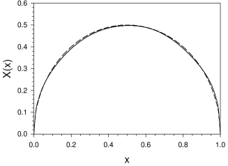
(a)
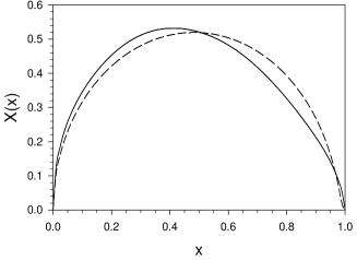
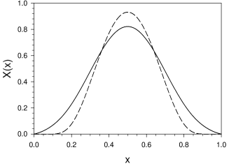
(b)	(c)

Figure 1: Longitudinal wave functions $X(x)$ for the (a) pion, (b) kaon, and (c) J/$\Psi$. The solid lines are wave functions from our model; the dashed lines show the ansatz by Brodsky and De Téramond ansatz .

The results for decay constants are included in Table 1. The values for the pion and kaon are consistent and in agreement with experiment. Our model value for the J/$\Psi$ is significantly closer to experiment than the value obtained from the longitudinal ansatz.

The parton distributions are plotted for comparison in Figure 2. The rough similarity of the wave functions translates into similar parton distributions.

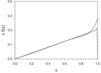
(a)
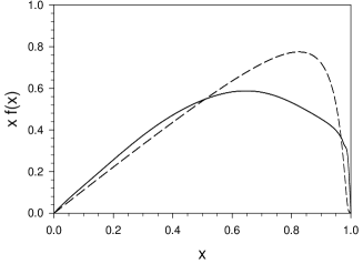
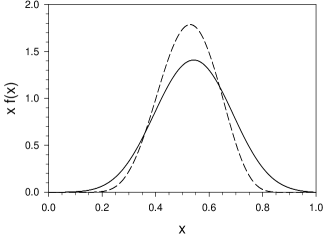
(b)	(c)

Figure 2: Same as Fig. 1 but for parton distributions $f(x)$ multiplied by $x$.

V Concluding remarks

We have constructed and solved a relativistic light-front equation for the longitudinal wave functions of mesons with massive quarks, to be used in tandem with the transverse equation of light-front holographic QCD. Comparisons with the ansatz ansatz (8) show that for lighter mesons, the longitudinal wave functions are quite similar. However, for the J/$\Psi$, there is a notable difference, which translates into a better estimate of the decay constant, as listed in Table 1. Wave functions for the J/$\Psi$, and also the pion and kaon, are shown in Fig. 1, and parton distributions are shown in Fig. 2. The similarity of the longitudinal wave functions provides the ansatz with a connection to the fundamental interactions of QCD.

Perhaps the most broadly useful outcome of this exercise is to illustrate that there is a convenient set of basis functions for longitudinal wave functions of meson valence states. These are the $f_{n}$ defined in (34), with the parameters $\beta_{i}$ to be optimized as needed for a given application. One could, of course, use the eigenfunctions of the ’t Hooft model, but these do not have an analytic form and would add an extra layer of complication to any calculation.

The importance of the choice of basis functions is in the rate of convergence as the basis is expanded. For the alternative of discrete light-cone quantization, it is known that convergence can be much slower vandesande . Thus, these basis functions may prove useful for calculations, such as those described in Vary , which use the transverse light-front holographic eigenfunctions.

Appendix A Light-front coordinates

Our conventions for light-front coordinates Dirac ; DLCQreviews are as follows. We define light-front time $x^{+}=t+z$ and the longitudinal light-front spatial coordinate $x^{-}=t-z$. The transverse coordinates are collected as $\vec{x}_{\perp}=(x,y)$. The corresponding light-front energy and momentum are $p^{-}=E-p_{z}$, $p^{+}=E+p_{z}$, and $\vec{p}_{\perp}=(p_{x},p_{y})$. From the invariant mass relation $m^{2}=p^{2}=p^{+}p^{-}-\vec{p}_{\perp}^{2}$, we obtain $p^{-}=(m^{2}+p_{\perp}^{2})/p^{+}$ for an on-shell particle.

For a system of particles, with total momentum $(P^{+},\vec{P}_{\perp})$, the longitudinal momentum fraction $x_{i}=p_{i}^{+}/P^{+}$ and relative transverse momentum $\vec{k}_{\perp i}=\vec{p}_{\perp i}-x_{i}\vec{P}_{\perp}$, for the ith particle, are boost invariant and therefore a convenient choice for independent variables in the description of the system. They sum to one and zero, respectively:

$$\sum_{i}x_{i}=1,\;\;\;\;\sum_{i}\vec{k}_{\perp i}=0.$$ (23)

The invariant mass for the system is

$$P^{+}\sum_{i}p_{i}^{-}-\vec{P}_{\perp}^{2}=\sum_{i}\frac{m_{i}^{2}+(x_{i}\vec{P}_{\perp}+\vec{k}_{\perp i})^{2}}{p_{i}^{+}/P^{+}}-\vec{P}_{\perp}^{2}=\sum_{i}\frac{m_{i}^{2}+\vec{k}_{\perp i}^{2}}{x_{i}}.$$ (24)

For a two-particle system, the internal variables reduce to $x=x_{1}$, $x_{2}=1-x$, $\vec{k}_{\perp}=\vec{k}_{\perp 1}$, and $\vec{k}_{\perp 2}=-\vec{k}_{\perp}$, and the invariant mass becomes

$$\frac{m_{1}^{2}+\vec{k}_{\perp 1}^{2}}{x_{1}}+\frac{m_{2}^{2}+\vec{k}_{\perp 2}^{2}}{x_{2}}=\frac{m_{1}^{2}}{x}+\frac{m_{2}^{2}}{1-x}+\frac{\vec{k}_{\perp}^{2}}{x(1-x)}.$$ (25)

Appendix B Dual form-factor analysis

In the Drell–Yan–West frame DrellYan , the form factor for momentum transfer $q^{2}$ can be written in terms of Fock-state wave functions $\psi_{n}$ as BrodskyDrell

$$F(q^{2})=\sum_{n}\int[dx_{i}][d^{2}k_{\perp i}]\sum_{j}e_{j}\psi_{n}^{*}(x_{i},\vec{k}_{\perp i}^{\,\prime})\psi_{n}(x_{i},\vec{k}_{\perp i}),$$ (26)

where $n$ denotes the Fock sector, $e_{j}$ the charge of the $j$th quark,

$$[dx_{i}]\equiv\prod_{i=1}^{n}\int dx_{i}\delta(1-\sum_{j}x_{j}),$$ (27)

$$[d^{2}k_{\perp i}]\equiv\left(\prod_{i=1}^{n}\int\frac{d^{2}k_{\perp i}}{16\pi^{3}}\right)16\pi^{3}\delta(\sum_{j}\vec{k}_{\perp j}),$$ (28)

and, with $j$ the index of the quark that absorbed the photon,

$$\vec{k}_{\perp i}^{\,\prime}=\left\{\begin{array}[]{ll}\vec{k}_{\perp i}+(1-x)\vec{q}_{\perp},&i=j\\ \vec{k}_{\perp i}-x\vec{q}_{\perp},&i\neq j.\end{array}\right.$$ (29)

Substitution of the wave function as a transverse Fourier transform in impact space,

$$\psi_{n}(x_{i},\vec{k}_{\perp i})=(4\pi)^{(n-1)/2}\prod_{i=1}^{n-1}\int d^{2}b_{\perp i}e^{i\sum_{j=1}^{n-1}\vec{b}_{\perp j}\cdot\vec{k}_{\perp j}}\widetilde{\psi}_{n}(x_{i},\vec{b}_{\perp i}),$$ (30)

converts the expression (26) for the form factor to

$$F(q^{2})=\sum_{n}\prod_{j=1}^{n-1}\int dx_{j}d^{2}b_{\perp j}e^{i\vec{q}_{\perp}\cdot\sum_{j=1}^{n-1}x_{j}\vec{b}_{\perp j}}|\widetilde{\psi}_{n}(x_{i},\vec{b}_{\perp i})|^{2}.$$ (31)

For the quark-antiquark valence sector alone, with the wave function given by $\widetilde{\psi}_{2}=e^{iL\varphi}X(x)\phi(\zeta)/\sqrt{2\pi\zeta}$, this reduces to

$$F(q^{2})=\int\frac{dx\,|X(x)|^{2}}{x(1-x)}\int d\zeta J_{0}\left(\zeta q_{\perp}\sqrt{x/(1-x)}\right)|\phi(\zeta)|^{2},$$ (32)

with $J_{0}$ the Bessel function of order zero. This is to be compared with the form computed in AdS₅ PolchinskiStrassler

$$F(q^{2})=\int dx\int d\zeta J_{0}\left(\zeta q_{\perp}\sqrt{x/(1-x)}\right)|\phi(\zeta)|^{2}.$$ (33)

Thus, the conclusion LFhQCD that $X(x)=\sqrt{x(1-x)}$, when the quarks have zero current mass.

Appendix C Numerical solution

We solve (11) numerically by expanding the wave function $X$ in terms of orthonormal basis functions $f_{n}$, chosen to include the analytic approximation explicitly. As discussed by Mo and Perry MoPerry , these basis functions are

$$f_{n}(x)=N_{n}x^{\beta_{1}}(1-x)^{\beta_{2}}P_{n}^{(2\beta_{2},2\beta_{1})}(2x-1),$$ (34)

with $P_{n}^{(2\beta_{2},2\beta_{1})}$ the Jacobi polynomial of order $n$. The normalization factor $N_{n}$ is given by AbramowitzStegun

$$N_{n}=\sqrt{(2n+2\beta_{1}+2\beta_{2})\frac{n!\Gamma(n+2\beta_{1}+2\beta_{2}+1)}{\Gamma(n+2\beta_{1}+1)\Gamma(n+2\beta_{2}+1)}}.$$ (35)

The solution is then represented as

$$X(x)=\sum_{n}c_{n}f_{n}(x).$$ (36)

For equal-mass cases, the longitudinal equation obeys an $x\leftrightarrow(1-x)$ symmetry, and only the even-$n$ terms will contribute. In general, we find that only a few terms are needed; the $n=0$ term, for which the Jacobi polynomial is constant and $f_{0}\propto x^{\beta_{1}}(1-x)^{\beta_{2}}$, represents 90% or more of the probability.

The expansion coefficients $c_{n}$ are obtained by diagonalizing the longitudinal equation in the $f_{n}$ basis. The matrix representation is

$$\left(\frac{m_{1}^{2}}{m_{u}^{2}}A_{1}+\frac{m_{2}^{2}}{m_{u}^{2}}A_{2}+B\right)\vec{c}=\xi\vec{c},$$ (37)

with $\xi\equiv C/m_{u}^{2}$ and matrices $A_{1}$, $A_{2}$, and $B$ defined by

$$(A_{1})_{nm} = \int_{0}^{1}\frac{dx}{x}f_{n}(x)f_{m}(x),\;\;(A_{2})_{nm}=\int_{0}^{1}\frac{dx}{1-x}f_{n}(x)f_{m}(x),$$ (38)

$$B_{nm} = \int_{0}^{1}dx\,{\cal P}\!\!\int_{0}^{1}dyf_{n}(x)\frac{f_{m}(x)-f_{m}(y)}{(x-y)^{2}}.$$ (39)

Following ’t Hooft tHooft , the matrix representation is made explicitly symmetric by rewriting the potential term as

$$B_{nm}=\frac{1}{2}\int_{0}^{1}dx\int_{0}^{1}dy\frac{f_{n}(x)-f_{n}(y)}{x-y}\frac{f_{m}(x)-f_{m}(y)}{x-y}.$$ (40)

In addition to the explicit symmetry, which simplifies the matrix diagonalization, this rearrangement also resolves the principal value prescription. The matrices are small because the number of terms needed in the expansion are few; the diagonalization is then straightforward.

References

- (1) S.J. Brodsky and G.F. de Téramond, Phys. Rev. Lett. 96 (2006), 201601.
- (2) J. Polchinski and M.J. Strassler, Phys. Rev. Lett. 88 (2002), 031601; JHEP 05 (2003), 012.
- (3) S.J. Brodsky and G.F. de Téramond, Phys. Rev. D 77 (2008), 056007.
- (4) S.J. Brodsky and G.F. de Téramond, Phys. Lett. B 582 (2004), 211; J. Erlich, E. Katz, D.T. Son, and M.A. Stephanov, Phys. Rev. Lett. 95, 261602 (2005); Z. Abidin and C.E. Carlson, Phys. Rev. D 77 (2008), 095007; S.J. Brodsky and G.F. de Téramond, Phys. Rev. 78 (2008), 025032; G.F. de Téramond and S.J. Brodsky, Phys. Rev. Lett. 102 (2009), 081601.
- (5) A. Karch, E. Katz, D.T. Son, and M.A. Stephanov, Phys. Rev. D 74 (2006), 015005.
- (6) S.S. Gershtein, A.K. Likhoded, and A.V. Luchinsky, Phys. Rev. D 74 (2006), 016002.
- (7) A. Vega, I. Schmidt, T. Branz, T. Gutsche, and V.E. Lyubovitskij, Phys. Rev. 80 (2009), 055014.
- (8) D. Ebert, R.N. Faustov, and V.O. Galkin, Eur. Phys. J. C 66 (2010), 197.
- (9) T. Branz, T. Gutsche, V.E. Lyubovitskij, I. Schmidt, and A. Vega, Phys. Rev. D 82 (2010), 074022; T. Gutsche, V.E. Lyubovitskij, I. Schmidt, and A. Vega, Phys. Rev. D 85 (2012), 076003.
- (10) T.M. Kelley, S.P. Bartz, and J. Kapusta, Phys. Rev. D 83 (2011), 016002.
- (11) S.J. Brodsky and G.F. de Téramond, arXiv:0802.0514.
- (12) G. ’t Hooft, Nucl. Phys. B 75 (1974), 461.
- (13) W.A. Bardeen and R.B. Pearson, Phys. Rev. D 14 (1976), 547.
- (14) W.A. Bardeen, R.B. Pearson, and E. Rabinovici, Phys. Rev. D 21 (1980), 1037.
- (15) E. Katz and T. Okui, JHEP 901 (2009), 013.
- (16) G.F. de Téramond and S.J. Brodsky, AIP Conf. Proc. 1296 (2010), 128.
- (17) G.F. de Téramond and S.J. Brodsky, arXiv:1203.4025.
- (18) H. Bergknoff, Nucl. Phys. B 122 (1977), 215.
- (19) Y. Ma and J.R. Hiller, J. Comput. Phys. 82 (1989), 229.
- (20) Y. Mo and R.J. Perry, J. Comput. Phys. 108 (1993), 159.
- (21) S.J. Brodsky, T. Huang, and G.P. Lepage, Proceedings of the Banff Summer Institute on Particles and Fields 2, Banff, Alberta, 1981, edited by A.Z. Capri and A.N. Kamal (Plenum, New York, 1983), p. 143; G.P. Lepage, S.J. Brodsky, T. Huang, and P.B. Mackenzie, ibid., p. 83; T. Huang, AIP Conf. Proc. 68 (1980), 1000.
- (22) A.V. Radyushkin, Phys. Rev. D 58 (1998), 114008.
- (23) K. Nakamura et al.(Particle Data Group), J. Phys. G 37 (2010), 075021.
- (24) B. van de Sande, Phys. Rev. D 54 (1996), 6347.
- (25) J.P. Vary et al., Phys. Rev. C 81 (2010), 035205.
- (26) P.A.M. Dirac, Rev. Mod. Phys. 21 (1949), 392.
- (27) For reviews, see M. Burkardt, Adv. Nucl. Phys. 23 (2002), 1; S.J. Brodsky, H.-C. Pauli, and S.S. Pinsky, Phys. Rep. 301 (1998), 299.
- (28) S.D. Drell, D.J. Levy, and T.M. Yan, Phys. Rev. Lett. 22 (1969), 744; G.B. West, Phys. Rev. Lett. 24 (1970), 1206.
- (29) S.J. Brodsky and S.D. Drell, Phys. Rev. D 22 (1980), 2236.
- (30) M. Abramowitz and I.A. Stegun (eds.), Handbook of Mathematical Functions (Dover, New York, 1965).