Degree Relations of Triangles in Real-world Networks and Models

Abstract

Triangles are an important building block and distinguishing feature of real-world networks, but their structure is still poorly understood. Despite numerous reports on the abundance of triangles, there is very little information on what these triangles look like. We initiate the study of degree-labeled triangles — specifically, degree homogeneity versus heterogeneity in triangles. This yields new insight into the structure of real-world graphs. We observe that networks coming from social and collaborative situations are dominated by homogeneous triangles, i.e., degrees of vertices in a triangle are quite similar to each other. On the other hand, information networks (e.g., web graphs) are dominated by heterogeneous triangles, i.e., the degrees in triangles are quite disparate. Surprisingly, nodes within the top 1% of degrees participate in the vast majority of triangles in heterogeneous graphs. We also ask the question of whether or not current graph models reproduce the types of triangles that are observed in real data and showed that most models fail to accurately capture these salient features.

1 Introduction

There is a growing interest in understanding the structure, dynamics, and evolution of large scale networks. Observing the commonalities and differences among real-world networks improves graph mining in many aspects ranging from community detection to generation of more realistic random graphs.

A triangle is a set of three vertices that are pairwise connected and is arguably one of the most important patterns in terms of understanding the inter-connectivity of nodes in real graphs [13, 34]. Note that the community structure is closely tied to triangles, and the degree behavior of triangles is an integral part of this structure [30]. Whether these graphs come from communication networks, social interaction, or the Internet, the presence of triangles is indication of community behavior. In social networks, it is considered highly probable that friends of friends will themselves be friends, thus forming many triangles. Social scientists have long observed the significance of triangles, as they are manifestations of specific interaction patterns [11, 27, 35, 7, 17]. For example, in friendship networks, a significant difference among degrees in triangle vertices might indicate an anomaly such as existence of a spam bot [3].

In this paper, we take a closer look at the structure of triangles, specifically, the degrees of the triangle vertices. Consider the two triangles in Figure 1. How are the degrees of the three vertices related? Do these represent fundamentally different types of relationships and so appear in different sorts of networks? When we look at real-world networks, we may ask if there is a high incidence of degree homogeneity, wherein vertices of similar degree come together to form triangles? Or do triangles tend to show degree heterogeneity, i.e., connecting vertices of disparate degree?

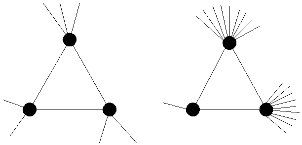
Figure 1: Homogeneity versus heterogeneity in triangles. The triangle on the left is homogeneous since degrees of all its vertices are close, and the one on the right is heterogeneous due to a mixture of high and low degree vertices.

1.1 Background and Previous Work

The study of triangles is quite prevalent in the social sciences community. Coleman [11] and Portes [27] used the clustering coefficient to predict the likelihood of going against social norms. Welles et al. studied the variance of clustering coefficients for different demographics groups and found that adolescents are more likely to have connected friends than adults and are even more likely to terminate connections with friends that are not connected to their other friends [35]. Burt underlined the importance of nodes that could serve as a bridge between various communities [6] and tied this to the number of open triangles in a vertex [7]. Lawrence [17] observed that there are powerful homophily effects in who connects to whom in organizational environments, who people are aware of, or whose opinions people attend to. Bearman, Moody, and Stovel studied homogeneity of partners in a romantic network of adolescents [2]. One noteworthy observation in this study was the similarity on partnership experience, which corresponds to similarity in vertex degrees.

The notion of describing graph structure based on the frequency of small patterns such as triangles has been proposed under different names such as motifs [5, 24], graphlets [28], and structural signatures [12]. Triangle counts form the basis for community detection algorithms in [4, 14]. They have also served as the driving force for generative models [30, 34]. Eckman and Moses [13] interpreted the clustering coefficients as a curvature and showed that connected regions of high curvature on the WWW characterized common topics. Directed triangles are important motifs for comparing and characterizing graphs [5, 12, 22, 23, 28]. For graph databases, exploiting frequent patterns have also been proposed for efficient query processing [32, 37].

The frequency of triangles is often measured using the clustering coefficient, as defined by Watts and Strogatz [34]. We first establish some notation. Consider an undirected graph $G$ with $n$ vertices. Let $d_{j}$ denote the degree of node $j$ and $t_{j}$ denote the number of triangles containing node $j$. If we define a wedge to be a path of length 2, then the number of wedges centered at node $j$ is ${d_{j}\choose 2}$. Now we can define various clustering coefficients. The clustering coefficient of vertex $j$, $C_{j}$, is defined as the number of triangles incident to $j$ divided by the number of wedges centered at $j$, i.e., $C_{j}=t_{j}/{d_{j}\choose 2}$. The average of clustering coefficients across all vertices (called the local clustering coefficient) is defined as $\overline{C}=\frac{1}{n}\sum_{j}C_{j}$. Let $V_{d}=\{j:d_{j}=d\}$ be the set of vertices of degree $d$. We define the clustering coefficient of degree $d$ to be $C_{d}=\frac{1}{|V_{d}|}\sum_{j\in V_{d}}C_{j}$.

The (global) clustering coefficient, also known as the transitivity, is

$$C=\frac{3\times\text{total number of triangles}}{\text{total number of wedges}}=\frac{\sum_{j}t_{j}}{\sum_{j}{d_{j}\choose 2}}.$$

For random graphs with no structure, $C$ and $\overline{C}$ values are extremely small [26].

Most of the studies on degree-based similarity is based on assortativity, which was introduced by Newman [25]. Various studies have been conducted on the assortativity (or lack thereof) of real graphs [15, 21, 36]. However, Newman’s assortativity measure is misleading to classify networks with heavy-tailed degree distributions because it produces either neutral or negative assortativity (disassortativity) values for most of the large scale networks as shown in Table 1 with $r$ values.

Most relevant to our work is that of Tsourakakis [33], which observed various power laws in triangle behavior. This work focused on triangle counts for nodes (how many triangles a node participates). He finds that the average number of triangles per vertices of a given degree follows a power-law distribution and the slope of the degree-triangle plot has the negative slope of the degree distribution plot of the corresponding graph. It is argued that low degree nodes form fewer triangles than higher degree nodes. Our analysis shows that while this is certainly true for social networks, it does not hold for information networks, such as the autonomous systems networks.

1.2 Contributions

Our contributions fall into two categories. Our first set of results comes from empirical studies of degree relations in triangles of real graphs. Then, we perform experiments on a variety of graph models to show their (in)ability to reproduce the behavior of real graphs.

Triangle homogeneity vs heterogeneity: We take a collection of graphs from diverse scenarios (collaboration, social networking, web, infrastructure) and measure triangle degree relationships. We compute various correlations between degrees of vertices in triangles to understand the homogeneity nature of these triangles.

Our experiments showed that graphs coming from social or collaborative scenarios are completely dominated by homogeneous triangles. There are a few heterogeneous triangles. This may not be surprising from a sociological viewpoint, since like should attract like. But graphs coming from web, routing, or communication are dominated by heterogeneous triangles. It is interesting that in communication or routing networks, majority of triangles are formed by the vertices within top 1% degrees.

We observed that there is a high correlation between global clustering coefficient $C$ and the homogeneity tendency of triangles. The higher $C$ a network has, the stronger homogeneity tendency the network has.

We also showed that the triangles in networks have diverse degrees of vertices and there is a varying distance among triangle degrees.

The triangle behavior of graph models: Our result can be stated quite succinctly. No existing graph model reflects the homogeneous and heterogeneous triangle behavior together. Many standard graph models like Preferential Attachment, Edge Copying, Stochastic Kronecker, etc. do not generate enough triangles and they cannot approximate the clustering coefficients of the real graphs [29]. The Chung-Lu [8] model cannot generate homogeneous graphs and cannot approximate the clustering coefficient of the high clustering coefficient networks. However, Chung-Lu is the only model imitates the networks with low clustering coefficient and it is enable to generate heterogeneous triangles.

The Forest Fire [20] and BTER [30] models generate a reasonable number of triangles (especially incident to low degree vertices) but these triangles are extremely homogeneous. Low degree vertices, when they participate in triangles, exclusively form triangles with other low degree vertices. This happens regardless of parameter choices, and is a fundamental property of these models. This shows that while they can qualitatively look like social and interaction networks, the behavior of, say, heterogonous networks cannot be reproduced by these models.

Table 1: Properties of networks we analyzed.

	Graph Name	$N$	$E$	$\rho$	$C$	$\overline{C}$	$T$	$\alpha$	$\kappa_{90}$	$\kappa_{99}$	$d_{\rm{max}}$	r
high-$C$	amazon0312	400K	2,349K	5.9	0.260	0.41	3,686K	3.1	19	55	2747	-0.02
	ca-AstroPh	18K	198K	11	0.318	0.63	1,351K	1.52	56	145	504	0.2
	cit-HepPh	34K	420K	12	0.146	0.30	1,276K	1.53	56	147	846	0
	soc-Epinions1	76K	405K	5.3	0.066	0.228	1,624K	1.68	65	307	3044	-0.04
low-$C$	as-caida20071105	26K	53K	2	0.007	0.21	36K	1.52	12	99	2628	-0.19
	oregon1_010331	10K	22K	2.1	0.009	0.45	17K	1.5	10	839	2312	-0.18
	web-Stanford	281K	1,992K	7.1	0.009	0.61	11,329K	1.51	30	92	38625	-0.11
	wiki-Talk	2,394K	4,659K	1.9	0.002	0.20	9,203K	1.67	21	401	100029	-0.06

2 Real-World Triangle Behavior

2.1 Data

We analyze the degree relations among vertices of triangles on a diverse set of real-world graphs: collaboration network (ca-AstroPh), citation network (cit-HepPh), trust network (soc-Epinions1), co-purchasing network (Amazon0312), autonomous systems (as-caida20071105), routing network (oregon1_010331), web network (web-Stanford), and communication network (wiki-Talk). All these graphs were obtained from the SNAP database [38]. In our studies, we have symmetrized the graphs by treating all edges as undirected; made each graph simple, by removing self loops and parallel edges; and did not use edge weights. Cohen’s algorithm [10] was used to enumerate all triangles.

In Table 1, we provide the following properties of the graphs we analyzed: $N$ = number of nodes; $E$ = number of edges; $\rho=E/N$ (density); $C$ = global clustering coefficient; $\overline{C}$ = local clustering; $T$ = number of triangles; $\alpha$ = the power-law exponent, which is computed by fitting power-law distribution to degree distribution plots of the graphs [9]; $\kappa_{90}$ and $\kappa_{99}$, respectively, are the 90th and 99th percentiles of degree of all nodes participating in triangles (i.e., we obtain all nodes participating in any triangle (each node is only counted once), put their degrees in a list, and then pick the 99th percentile of the degree list); $d_{\rm{max}}$ = maximum degree; and $r$ = assortativity value.

In this paper, a network whose global clustering coefficient, $C$ is greater than 0.01, is referred to as a high-$C$ network, and as a low-$C$ network otherwise. In Table 1, the first 4 graphs are high-$C$ graphs, whereas the last 4 are low-$C$ graphs.

2.2 Analysis

We analyze the degree similarity of triangle vertices by grouping the triangles according to their minimum degree vertex. We first present the notation. For $t=1,\dots,T$, let $d_{\rm min}{(t)}$, $d_{\rm mid}{(t)}$, and $d_{\rm max}{(t)}$ denote the minimum, middle, and maximum degree of the $t$-th triangle. For instance, if the $t$-th triangle has vertices of degrees $5,10$, and $4$, then $d_{\rm min}{(t)}=4$, $d_{\rm mid}{(t)}=5$, and $d_{\rm max}{(t)}=10$. Define the set $\mathcal{B}({i})$ to be the set of all triangles whose minimum degree is $i$, i.e.,

$$\mathcal{B}({i})=\Set{t\in T}{d_{\rm min}{(t)}=i}.$$

We may then define some average statistics for each set $\mathcal{B}({i})$. Define $d_{1}{(i)}$, $d_{2}{(i)}$, and $d_{3}{(i)}$ to be the median of minimum, middle, and maximum degree, respectively, of triangles in $\mathcal{B}({i})$. In other words,

$$d_{1}{(i)} ={\rm median}\Set{d_{\rm min}{(t)}}{t\in\mathcal{B}({i})}=i,$$

$$d_{2}{(i)} ={\rm median}\Set{d_{\rm mid}{(t)}}{t\in\mathcal{B}({i})},$$

$$d_{3}{(i)} ={\rm median}\Set{d_{\rm max}{(t)}}{t\in\mathcal{B}({i})}.$$

For instance, if the triangles in $\mathcal{B}({2})$ were given by $[2\ 2\ 3]$, $[2\ 4\ 5]$, and $[2\ 3\ 3]$. Then, the $d_{1}{(2)}=2$, $d_{2}{(2)}=3$ and $d_{3}{(2)}=3$.

To compare the relations among triangle degrees, we plot the $d_{2}{(i)}$ and $d_{3}{(i)}$ versus $d_{1}{(i)}$ as in Figure 2 and call them degree-comparison plots. Note that in these and all other log-log and semi-log plots, we use the exponential binning which is a standard procedure to de-noise the data when plotting on logarithmic scale.

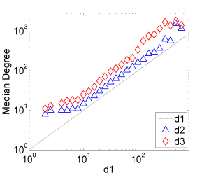
(a) amazon0312

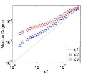
(b) ca-AstroPh

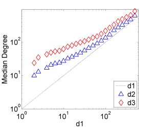
(c) cit-HepPh

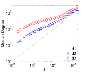
(d) Soc-Epinions

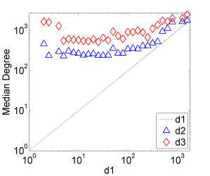
(e) as-caida20071105

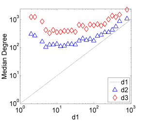
(f) oregon1_010331

(g) web-Stanford

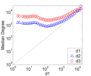
(h) wiki-Talk

Figure 2: Triangle degree-comparison plots which compare the medians of minimum degree, $d_{1}{(i)}$, the middle degree, $d_{2}{(i)}$, and the maximum degree $d_{3}{(i)}$

2.3 Observations

By considering the degree relations of the triangle vertices, we make the following observations.

Observation 1: The global clustering coefficient is an indicator for the triangle degree relations.

When we analyze Figure 2, we can see a clear relation between global clustering coefficient $C$ and the type of triangles. In high-$C$ networks, minimum, middle, and maximum degrees of triangle vertices are close in value. While, in low-$C$ networks, triangles are highly heterogeneous. Observe how very small values of $d_{1}{(i)}$ connect to quite large $d_{2}{(i)}$ or $d_{3}{(i)}$. In Figure 2e, Figure 2f and Figure 2h low degree vertices are connecting to two high vertices ($d_{2}{(i)}$ and $d_{3}{(i)}$). Web-Stanford (Figure 2g) is less structured and has a different tendency from the rest but it is still visible that low degree vertices are connecting to high $d_{3}{(i)}$ value.

The average clustering coefficient $\overline{C}$ is not a very distinguishing metric for our study. The global clustering coefficient $C$ shows wide variance and is a better indicative of the triangle behavior.

Observation 2: There is a non-trivial gap between the minimum, medium, and maximum degrees of triangles.

Even though the degrees of triangle vertices are similar to each other in high-$C$ networks, still there is a non-trivial between $d_{1}{(i)}$ and $d_{2}{(i)}$ and between $d_{2}{(i)}$ and $d_{3}{(i)}$ in Figure 2. This observation tells us that inside the communities or clusters in real networks, there exist triangles with varying degrees of vertices.

Observation 3: The ratios among degrees of triangle vertices are small in high-$C$ networks and large in low-$C$ networks.

The ratios of triangle degrees provide valuable information to see the distinction between networks. For the $t$-th triangle, three degree ratios are defined as follow: $r_{21}{(t)}=\frac{d_{\rm mid}{(t)}}{d_{\rm min}{(t)}}$, $r_{31}{(t)}=\frac{d_{\rm max}{(t)}}{d_{\rm min}{(t)}}$, and $r_{32}{(t)}=\frac{d_{\rm max}{(t)}}{d_{\rm mid}{(t)}}$. These ratios are computed for all the triangles separately and their average is computed as $\bar{r}_{21}$, $\bar{r}_{31}$, and $\bar{r}_{32}$, respectively. Table 2 lists the average ratios for all the networks.

Table 2: The average of triangle degree ratios

	Graph Name	$\bar{r}_{21}$	$\bar{r}_{31}$	$\bar{r}_{32}$
high-$C$	amazon0312	1.98	4.95	2.53
	ca-AstroPh	1.88	3.46	1.89
	cit-HepPh	2.20	4.96	2.38
	soc-Epinions1	3.34	9.41	2.95
low-$C$	as-caida20071105	70.99	164.35	8.14
	oregon1_010331	54.80	175.69	9.09
	web-Stanford	87.91	300.37	114.43
	wiki-Talk	42.64	138.01	4.75

There is a clear distinction between high-$C$ and low-$C$ networks. The average ratios are very small in high-$C$ networks, which also supports the triangle homogeneity in high-$C$ networks. The average of $\bar{r}_{21}$ and $\bar{r}_{32}$ are close to each other, in other words, the middle degree is both close to the minimum degree and the maximum degree.

The average degree ratios are significantly large in low-$C$ networks. Particularly, the ratio between the maximum and the minimum degree is very high. We can see that in as-caida20071105, oregon1_010331, wiki-Talk, middle and maximum degrees are close to each other but these degrees differ from the minimum degree significantly. Web-Stanford acts little different. In this graph, minimum and middle degrees are close to each other but the maximum degree is distant to both the minimum and the medium degrees.

We have also looked at the percentage of homogeneous triangles, which we define triangles where $\bar{r}_{31}<10$. Figure 3 shows that more than 90% of the triangles in high-$C$ networks are homogeneous.

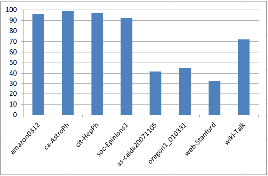
Figure 3: Percentage of triangles such that $d_{\max}/d_{\min}\leq 10$

Observation 4: In low-$C$ networks, high degree vertices within the top 1% participate in the vast majority of the triangles.

In high-$C$ networks, the triangles incident to low degree vertices are mostly connecting to two low degree vertices. On the other hand, in low-$C$ networks (particularly in the low density networks), a significant portion of the triangles contain at least one high degree vertex.

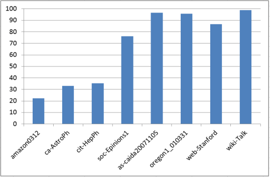
Figure 4: The percentage of triangles produced by vertices in the Top 1% degrees

To set a threshold between low degrees and high degrees, we have experimented different percentiles of vertices that participate in at least one triangle. In Table 1, $\kappa_{90}$, $\kappa_{99}$, and the maximum degree of each network are presented. It is interesting that the gap between $\kappa_{90}$ and $\kappa_{99}$ is quite large in low-$C$ networks. We pick $\kappa_{99}$ as a threshold, since $\kappa_{90}$ is still relatively low compared to the maximum degree in most networks. A degree of a triangle vertex is considered low, if the degree is no greater than $\kappa_{99}$, high otherwise it is considered.

We look at the percentages of the triangles having at least one high degree node in Figure 4. In low-$C$ networks, we can say that high degree vertices within the top 1% participate in most of the triangles. In high-$C$, high degree nodes are participating in less triangles except soc-Epinions network. Soc-Epinions has a very low clustering coefficient value (i.e., less than $0.1$) and it is a border case. Hence, its statistics are higher than the other high-$C$ networks.

3 Graph-Model Triangle Behavior

In this section, we investigate how well random graph generators match the real graphs in terms of triangle degree similarity. We concentrate on the graph models generating heavy-tailed degree distributions.

Table 3: The number of triangles generated by graph models

	Graph Name	Original	BTER	CL	FF	EC	PA	SKG
high-$C$	amazon0312	3,686K	3,704K	5K	4,420K	12K	10K	12K
	ca-AstroPh	1,351K	1,315K	49K	2,937K	43K	20K	4K
	cit-HepPh	1,276K	1,315K	48K	8,502K	180K	40K	34K
	soc-Epinions1	1,624K	2,128K	641K	1,199K	24K	4K	44K
low-$C$	as-caida20071105	36K	74K	43K	38K	3K	$\textless$ 1K	3K
	oregon1_010331	17K	26K	15K	17K	1K	$\textless$ 1K	$\textless$ 1K
	web-Stanford	11,329K	14,185K	3,783K	11,651K	158K	16K	114K
	wiki-Talk	9,203K	66,740K	41,427K	2,936K	16K	$\textless$ 1K	$\textless$ 1K

3.1 Graph Models

Barabasi-Albert [1] proposed the Preferential Attachment (PA) model is often associated with the “rich get richer" concept. In the PA model, a new node connects to a pre-specified number of vertices, where the likelihood of choosing a vertex is proportional to its degree. This procedure leads to graphs with power-law degree distributions. As Sala et al. [29] pointed out, PA model cannot create communities in the graph and cannot generate high clustering coefficients for low degree nodes.

The Stochastic Kronecker Graph (SKG) model [19] starts with a basis matrix (typically $2\times 2$), and generates a matrix that specifies edge probabilities by repeated Kronecker products. A noise-added version of SKG has been proven to generate log-normal degree distributions [31], but the clustering coefficients of SKG graphs are very low [26].

The Chung-Lu (CL) model [8] can be considered as picking a random graph among all graphs with the same degree distribution. In this model, the probability of an edge is proportional to the product of the degrees of its endpoints, (i.e., $Pr\left(e_{ij}\right)=\frac{d_{i}d_{j}}{\left(2m\right)^{2}}$). Pinar et al. showed that many properties of graphs generated by SKG and CL models are similar [26].

The Block Two-Level Erdős-Rényi (BTER) model [30] is built on the observation of high-clustering coefficients and skewed degree distributions. This model achieves high clustering coefficients by embedding communities with an Erdős-Rényi structure, which is typically much denser compared to the rest of the graph. Edges are added in a subsequent phase using the CL model, to satisfy the degree distribution requirements. It has been shown that BTER graphs can match many properties of real world graphs [30].

The Edge Copying (EC) model  [16] imitates the topic-based communities in the Web, and generates an evolving directed graph. When a new node arrives, it selects a random vertex and copies a specified number of links. For the EC model, both the in-degree and out-degree distributions follow power laws. However, the model does not create back links and does not generate many triangles.

The Forest Fire (FF) model [20] combines the PA model [1] to obtain a heavy-tailed degree distribution, the EC model  [16] to obtain communities, and community guided attachment for densification. The model has a forward burning parameter $p$. In the FF model, a node $v$ arrives and chooses an ambassador node $w$ randomly and connected to each neighbor of $w$ with probability $p$. This process is repeated for each new vertex $v$ connects to. Note that EC model only copies the links of a node, it does not hop to the neighbor of the node.

3.2 Fitting Graph Models to Real Networks

To check whether graph models can reproduce the triangle degree behavior of the real networks, we fit FF, BTER, EC, CL, PA, and SKG models to the real networks listed in Table 1.

The inputs to the The PA model are the number of nodes $n$ and the number of edges $k$ created by each node. We pick $k$ by rounding the density of the graph in order to match the number of edges in the real networks.

The BTER model takes the degree distribution of the real networks. The connectivity per block is computed by a table look-up on the average clustering coefficient per degree $C_{d}$ plot.

For the Chung Lu model, we provide the degree distribution of the real networks as an input to the model.

For the Forest Fire model, we provide the number of nodes $n$ and the forward burning probability $p$. We match the generated graph models to the number of edges in the real networks. For each target graph, we search a range of values by incrementing $p$ value by $\delta p=0.001$ in range [0-1] to find the best model giving the similar number of edges to the original network.

The EC model takes the number of nodes $n$, number of edges each node creates $k$, and the edge copying probability $p$ which is calculated based on power-law degree distribution. Power-law degree slope is $\frac{1}{1-p}$. We pick $k$ by rounding up the density of graph.

To generate the SKG model, we compute the parameters of the initiator matrix using the Kronfit algorithm [18]. The size of the final adjacency matrix is $2^{\lceil\log(n)\rceil}$ where $n$ is the number of nodes in the real graph.

Before running our experiments, we symmetrize by treating each edge as undirected and remove self-links for all the generated graphs.

3.3 Triangle Analysis in Graph Models

After fitting different graph models on the real networks, we enumerate triangles in each randomly generated network using Cohen’s algorithm [10]. We analyze the triangle behaviors in these random graphs in different aspects.

The numbers of triangles: None of the graph models capture the triangle numbers for both high-$C$ and low-$C$ networks.

Some models are good at generating similar number of triangles for high-$C$ networks, some of them are good at for low-$C$ networks, but none of them is good at both. The number of triangles generated by different graph models for each target graph is listed in Table 3. Graph models behave differently in high-$C$ and low-$C$ networks in terms of generating triangles.

In high-$C$ networks, BTER matches the number of triangles in the original graph better than the rest of the models. FF creates significantly more triangles than the original number of triangles. CL generates significantly less triangles than the original number of triangles. For networks with the high clustering coefficient $C$ and high density $\rho$, CL is not a good choice.

In low-$C$ networks, BTER generates more triangles than the original number of triangles. As a matter of fact, when the $C$ value is very small, BTER generates even more triangles than the original number of triangles. Particularly for wiki-Talk, it generates many more triangles. CL is also generating many more triangles for wiki-Talk. CL is generating less triangles for web-Stanford but it generates similar number of triangles for oregon1_010331 and as-caida20071105. FF generates similar numbers of triangles as in the original networks except wiki-Talk. It seems that none of the models can reproduce the structure of the wiki-Talk graph.

EC, PA, and SKG generate significantly less triangles than the original triangle numbers. These models also cannot reach the average clustering coefficient per degree for any of the network. Therefore, we will not include them for the rest of the plots.

Degree Relations: Models generate either homogenous or heterogonous triangles for graphs. In Figure 5, we show the relation between $d_{1}{(i)}$ and $d_{2}{(i)}$ and in Figure 6, we show the relation between $d_{1}{(i)}$ vs $d_{3}{(i)}$ for the real graphs as well as their modeled counterparts.

CL produces heterogeneous triangles for both high-$C$ and low-$C$ networks in both Figure 5 and Figure 6. For low-$C$ networks, it is very intriguing that CL graphs are generating the right type of triangles, since the $d_{1}{(i)}$ vs $d_{2}{(i)}$ and $d_{1}{(i)}$ vs $d_{3}{(i)}$ plots follow the true graph quite well. But we feel that this indicates that low-$C$ networks have a CL flavor to them (i.e., triangles are random).

BTER generates homogeneous triangles for both high-$C$ and low-$C$ networks. For high-$C$ networks, BTER matches the $d_{1}{(i)}$ vs $d_{2}{(i)}$ but generates lower $d_{3}{(i)}$ values than original $d_{3}{(i)}$ values.

FF behaves like BTER for low-$C$ networks in $d_{1}{(i)}$ vs $d_{2}{(i)}$ and $d_{1}{(i)}$ vs $d_{3}{(i)}$ plots. Low degree $d_{1}{(i)}$ values cannot connect to high degree vertices. For high-$C$ networks, there is a steep increase after $d_{1}{(i)}$ reaches $10$ in some of the networks in both $d_{1}{(i)}$ vs $d_{2}{(i)}$ and $d_{1}{(i)}$ vs $d_{3}{(i)}$ plots. Distance between FF’s $d_{2}{(i)}$ and original $d_{2}{(i)}$ and FF’s $d_{3}{(i)}$ and original $d_{3}{(i)}$ is considerable large. FF also reaches higher $d_{1}{(i)}$ values than the original $d_{1}{(i)}$ values.

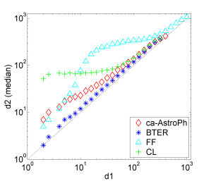
(a) ca-AstroPh

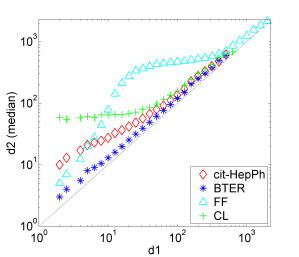
(b) cit-HepPh

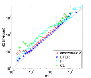
(c) Amazon0312

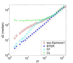
(d) Soc-Epinions

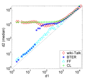
(e) wiki-Talk

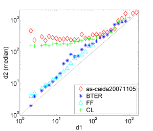
(f) as-caida20071105

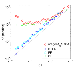
(g) oregon1_010331

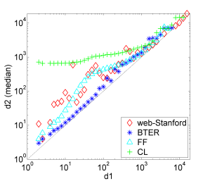
(h) web-Stanford

Figure 5: Triangle degree relations between $d_{1}{(i)}$ and $d_{2}{(i)}$ in the generated graph models

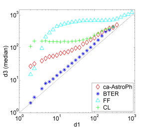
(a) ca-AstroPh

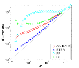
(b) cit-HepPh

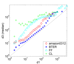
(c) Amazon0312

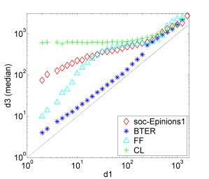
(d) Soc-Epinions

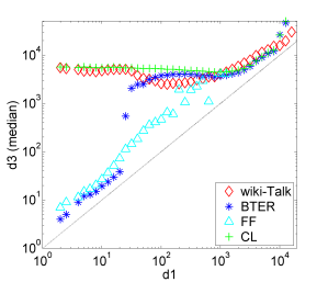
(e) wiki-Talk

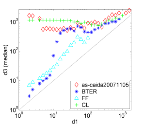
(f) as-caida20071105

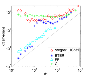
(g) oregon1_010331

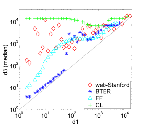
(h) web-Stanford

Figure 6: Triangle degree relations between $d_{1}{(i)}$ and $d_{3}{(i)}$ in the generated graph models

(a) ca-AstroPh

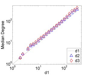
(b) ca-AstroPh BTER

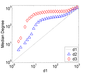
(c) ca-AstroPh FF

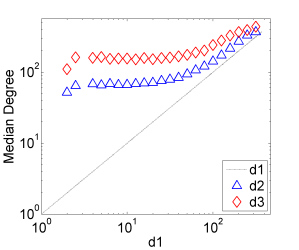
(d) ca-AstroPh CL

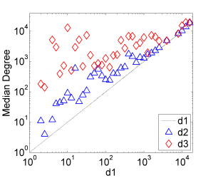
(e) web-Stanford

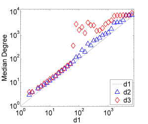
(f) web-Stanford BTER

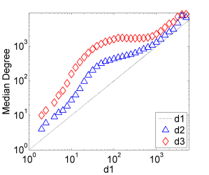
(g) web-Stanford FF

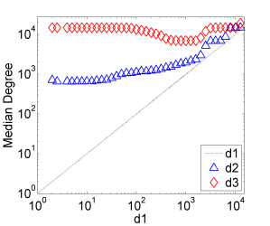
(h) web-Stanford CL

Figure 7: Triangle degree-comparison plots for the randomly generated graphs

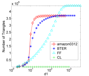
(a) amazon0312

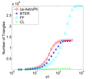
(b) ca-AstroPh

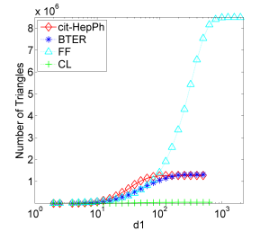
(c) cit-HepPh

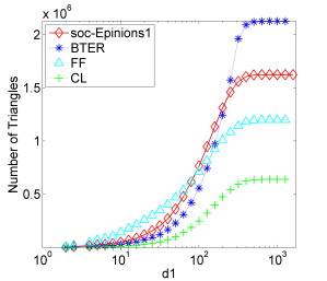
(d) soc-Epinions

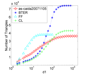
(e) as-caida20071105

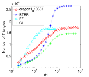
(f) oregon1_010331

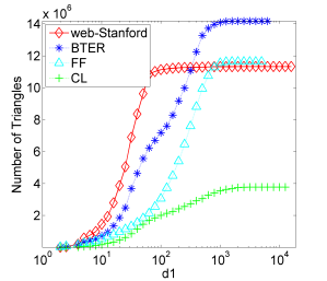
(g) web-Stanford

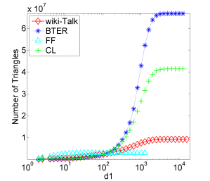
(h) wiki-Talk

Figure 8: Comparison of cumulative number of triangles for the different models

Distance Relations: Some models cannot provide a gap between minimum, medium, and maximum degrees of triangles.

We provide the degree-comparison plots of generated models in Figure 7 for one high-$C$ and one low-$C$ network as representative. The other networks in high-$C$ and low-$C$ networks have the similar degree-comparison plots.

For high-$C$ networks, BTER cannot provide the gap among minimum, middle, and maximum degrees. Having the almost same degree for all $d_{1}{(i)}$, $d_{2}{(i)}$, and $d_{3}{(i)}$ conflicts our Observation 2. FF provides a distance between minimum, middle, and maximum degrees, however, $d_{2}{(i)}$ and $d_{3}{(i)}$ strongly deviate from $d_{1}{(i)}$ in the middle (it generates a bump). CL also provides the gap among degrees but both $d_{2}{(i)}$ and $d_{3}{(i)}$ strongly deviates from $d_{1}{(i)}$ at the beginning.

For low-$C$ networks, BTER does not generate distance at the beginning again but in the middle it jumps to high $d_{3}{(i)}$ values. FF provides the gap but it has a bump in the middle again. CL provides much wider gap between $d_{2}{(i)}$ and $d_{3}{(i)}$.

It is very clear in Figure 7 that CL generates heterogonous triangles in any network, and FF and BTER generate more homogenous triangles and none of the graph models exactly match the triangle behavior in the original network.

The number of triangles per $d_{1}{(i)}$: None of the models obtain the number of triangles per $d_{1}{(i)}$ for both high-$C$ and low-$C$ networks.

To understand, how triangles are distributed among degrees, we analyze the number of triangles generated per minimum degree $d_{1}{(i)}$ for different graph models in Figure 8. Models behave differently for high-$C$ and low-$C$ networks again.

For high-$C$ networks, BTER model matches the original network behavior very well except Soc-Epinions (which is in the border of low-$C$). FF generates way too many triangles for high degree nodes except Soc-Epinions (it produces less triangles for this graph). CL is generating consistently lower number of triangles than the original number per minimum degree $d_{1}{(i)}$. For Soc-Epinions, CL generates slightly higher triangles but still less than the original. It is observable that when $C$ decreases, CL starts to generate comparably more triangles. In high-$C$ networks, FF reaches much higher $d_{1}{(i)}$ values (except Soc-Epinions). BTER and CL are reaching the similar $d_{1}{(i)}$ values to the real $d_{1}{(i)}$ .

For low-$C$ networks, none of the graph model matches to the original network behavior. BTER is generating more triangles for high degree nodes. CL is catching the similar behavior in Figure 8e and in Figure 8f but for the others it misses as well. FF tends to only generate triangles with relatively low degree vertices since the graphs are very sparse in low-$C$ networks. Hence, the plot for FF ends very early. In low-$C$ networks, FF reaches only one-tenth of the maximum $d_{1}{(i)}$ value of the original networks (except web-Stanford).

Clustering coefficient plots: The clustering coefficient behavior of models differ for high-$C$ and low-$C$ networks.

When we analyze average local clustering coefficient ($C_{d}$) per degree in graphs models as plotted in Figure 9, we can see the similar trends as in Figure 8. Clustering coefficient plots confirm that low degree vertices have high local clustering coefficient.

For high-$C$ networks, BTER matchs the local clustering coefficient behavior of the real graphs fairly well (in fact, the $C_{d}$ values are used as input to the model). FF is not matching perfectly but generates high $C_{d}$ values. CL is failing to reach high clustering coefficient values per degrees for high-$C$ networks but it has slightly better averages for low-$C$ networks.

For low-$C$ networks, BTER deviates from the original $C_{d}$ values in the middle. FF is not matching perfectly again but getting close. CL is generating higher $C_{d}$ averages than it generated for high-$C$ networks.

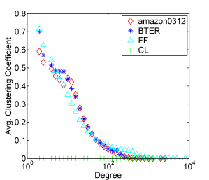
(a) amazon0312

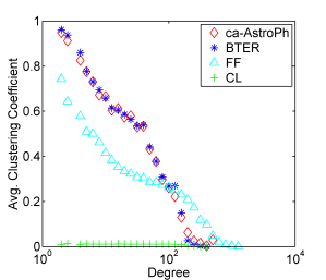
(b) ca-AstroPh

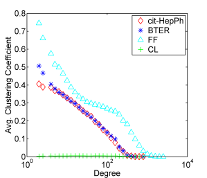
(c) cit-HepPh

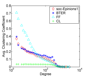
(d) soc-Epinions

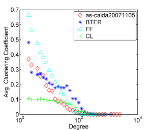
(e) as-caida20071105

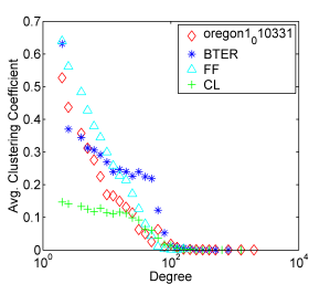
(f) oregon1_010331

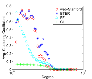
(g) web-Stanford

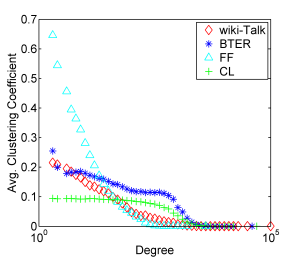
(h) wiki-Talk

Figure 9: Clustering Coefficient vs Degree Correlation for the different models

4 Conclusions

We believe that the dichotomy between homogeneous triangles and heterogeneous triangles is quite useful in characterizing graphs. This also gives a quantifiable method to distinguish the underlying processes creating these graphs. Social scientists and physicists have long tried to explain the behavior of humans (or appropriate agents) based on topological structure. The degree-labeled triangles appears to give us a window into this behavior.

The degree-labeled triangle behavior yields fascinating insight into the structure of real-world networks. As expected the triangles come in various types in different networks. However, our studies showed that the global clustering coefficient is a good indicator of what kind of triangles the graph contains. High clustering coefficients ($>0.01$) imply homogenous triangles (i.e., degrees of the vertices are close), while low clustering coefficients is a sign of heterogenous triangles (i.e., significant variance among the degrees of the vertices).

We have also investigated whether the current graph models can regenerate the types of triangles in the real data. The results showed that while some models are good at matching the total number of triangles in the real graph, no model can match the types of triangles for both the high and low clustering coefficient graphs together. Our paper shows that community structures in graph models are not able to capture the community behaviors in the real networks. Therefore, there is a room to improve the existent models and design more realistic graph models which support triangle degree behaviors.

References

- [1] Barabási, A.-L., and Albert, R. Emergence of scaling in random networks. Science 286, 5349 (1999), 509–512.
- [2] Bearman, P. S., Moody, J., and Stovel, K. Chains of Affection: The Structure of Adolescent Romantic and Sexual Networks. American Journal of Sociology 110, 1 (July 2004), 44–91.
- [3] Becchetti, L., Boldi, P., Castillo, C., and Gionis, A. Efficient semi-streaming algorithms for local triangle counting in massive graphs. In KDD’08 (2008), pp. 16–24.
- [4] Berry, J. W., Hendrickson, B., LaViolette, R. A., and Phillips, C. A. Tolerating the community detection resolution limit with edge weighting. Phys. Rev. E 83 (May 2011), 056119.
- [5] Boccaletti, S., Latora, V., Moreno, Y., Chavez, M., and Hwang, D.-U. Complex networks: Structure and dynamics. Physics Reports 424 (2006), 175–308.
- [6] Burt, R. S. Structural holes and good ideas. American Journal of Sociology 110, 2 (2004), 349–399.
- [7] Burt, R. S. Secondhand brokerage: Evidence on the importance of local structure for managers, bankers, and analysts. Academy of Management Journal 50 (2007).
- [8] Chung, F., and Lu, L. The average distances in random graphs with given expected degrees. PNAS 99 (2002), 15879–15882.
- [9] Clauset, A., Shalizi, C. R., and Newman, M. E. J. Power-law distributions in empirical data. SIAM Review 51, 4 (2009), 661–703.
- [10] Cohen, J. Graph twiddling in a MapReduce world. Computing in Science & Engineering 11 (2009), 29–41.
- [11] Coleman, J. S. Social capital in the creation of human capital. American Journal of Sociology 94 (1988), S95–S120.
- [12] Contractor, N. S., Wasserman, S., and Faust, K. Testing multitheoretical organizational networks: An analytic framework and empirical example. Academy of Management Review 31, 3 (2006), 681–703.
- [13] Eckmann, J.-P., and Moses, E. Curvature of co-links uncovers hidden thematic layers in the World Wide Web. PNAS 99, 9 (2002), 5825–5829.
- [14] Gleich, D. F., and Seshadhri, C. Neighborhoods are good communities. arXiv:1112.0031v1, 2011.
- [15] Holme, P., and Zhao, J. Exploring the assortativity-clustering space of a network’s degree sequence. Phys. Rev. E 75 (Apr 2007), 046111.
- [16] Kleinberg, J. M., Kumar, R., Raghavan, P., Rajagopalan, S., and Tomkins, A. S. The web as a graph: measurements, models, and methods. In Proceedings of the 5th annual international conference on Computing and combinatorics (Berlin, Heidelberg, 1999), COCOON’99, Springer-Verlag, pp. 1–17.
- [17] Lawrence, B. S. Organizational reference groups: A missing perspective on social context. Organization Science 17, 1 (2006), 80–100.
- [18] Leskovec, J., Chakrabarti, D., Kleinberg, J., Faloutsos, C., and Ghahramani, Z. Kronecker graphs: An approach to modeling networks. J. Machine Learning Research 11 (Feb. 2010), 985–1042.
- [19] Leskovec, J., and Faloutsos, C. Scalable modeling of real graphs using Kronecker multiplication. In ICML ’07 (2007), ACM, pp. 497–504.
- [20] Leskovec, J., Kleinberg, J., and Faloutsos, C. Graphs over time: densification laws, shrinking diameters and possible explanations. In Proceedings of the eleventh ACM SIGKDD international conference on Knowledge discovery in data mining (New York, NY, USA, 2005), KDD ’05, ACM, pp. 177–187.
- [21] Litvak, N., and van der Hofstad, R. Large scale-free networks are not disassortative. arXiv:1204.0266v1.
- [22] Mahadevan, P., Hubble, C., Krioukov, D. V., Huffaker, B., and Vahdat, A. Orbis: Rescaling degree correlations to generate annotated internet topologies. SIGCOMM’07 (2007), 325–336.
- [23] Mahadevan, P., Krioukov, D., Fall, K., and Vahdat, A. Systematic topology analysis and generation using degree correlations. SIGCOMM’06 (2006), 135–146.
- [24] Milo, R., Shen-Orr, S., Itzkovitz, S., Kashtan, N., Chklovskii, D., and Alon, U. Network motifs: Simple building blocks of complex networks. Science 298, 5594 (2002), 824–827.
- [25] Newman, M. E. J. Assortative mixing in networks. Phys. Rev. Letter 89 (May 20 2002), 208701.
- [26] Pinar, A., Seshadhri, C., and Kolda, T. G. The similarity between Stochastic Kronecker and Chung-Lu graph models. In Proceedings of SIAM Conference on Data Mining (2012), SIAM. arXiv:1110.4925, to appear in Proc. SDM12.
- [27] Portes, A. Social capital: Its origins and applications in modern sociology. Annual Review of Sociology 24, 1 (1998), 1–24.
- [28] Pr ulj, N. Biological network comparison using graphlet degree distribution. Bioinformatics 23, 2 (2007), e177–e183.
- [29] Sala, A., Cao, L., Wilson, C., Zablit, R., Zheng, H., and Zhao, B. Y. Measurement-calibrated graph models for social network experiments. In WWW ’10 (2010), ACM, pp. 861–870.
- [30] Seshadhri, C., Kolda, T. G., and Pinar, A. Community structure and scale-free collections of Erdős-Rényi graphs. Physical Review E 85 (May 2012).
- [31] Seshadhri, C., Pinar, A., and Kolda, T. Choosing parameters for stochastic kronecker graphs. In ICDM 2011 (2011).
- [32] Shasha, D., Wang, J. T.-L., and Giugno, R. Algorithmics and applications of tree and graph searching. In PODS’02 (2002), pp. 39–52.
- [33] Tsourakakis, C. Fast counting of triangles in large real networks without counting: Algorithms and laws. In ICDM’08 (2008), pp. 608–617.
- [34] Watts, D., and Strogatz, S. Collective dynamics of ‘small-world’ networks. Nature 393 (1998), 440–442.
- [35] Welles, B. F., Van Devender, A., and Contractor, N. Is a friend a friend?: Investigating the structure of friendship networks in virtual worlds. In CHI-EA’10 (2010), pp. 4027–4032.
- [36] Whitney, D. E., and Alderson, D. Are technological and social networks really different? 2006, pp. 25–30.
- [37] Yan, X., Yu, P. S., and Han, J. Graph indexing: A frequent structure-based approach. In SIGMOD’04 (2004), pp. 335–346.
- [38] Stanford Network Analysis Project (SNAP). Available at http://snap.stanford.edu/.