Half-metallic magnetization plateaux

Abstract

We propose a novel interaction-based route to half-metal state for interacting electrons on two-dimensional lattices. Magnetic field applied parallel to the lattice is used to tune one of the spin densities to a particular commensurate with the lattice value in which the system spontaneously ‘locks in’ via van Hove enhanced density wave state. Electrons of opposite spin polarization retain their metallic character and provide for the half-metal state which, in addition, supports magnetization plateau in a finite interval of external magnetic field. Similar half-metal state is realized in the finite-U Hubbard model on a triangular lattice at $1/3$ of the maximum magnetization.

Spin systems supporting robust magnetization plateaux whereby macroscopic magnetization $M$ is fixed at a rational fraction of the full (saturated) magnetization value $M_{\rm sat}$ in a finite interval of external magnetic field $h_{1}<h<h_{2}$ are subject of intense experimental studies Kodama et al. (2002); Kikuchi et al. (2005); Ueda et al. (2005); Fortune et al. (2009); Nema et al. (2009). Typically these materials are magnetic insulators which are well described by the Heisenberg-type models with short-range exchange interactions between localized spins.

One of the best understood and studied plateau states is represented by the up-up-down (UUD) magnetization plateau at $M=\frac{1}{3}M_{\rm sat}$ in the triangular lattice antiferromagnet Kawamura and Miyashita (1985); Chubukov and Golosov (1991). This 1/3 magnetization plateau is a remarkably stable state – it is known to survive significant spatial deformation of exchange integrals in both quantum (spin 1/2) and classical versions of the model Alicea et al. (2009); Griset et al. (2011), well beyond the point where adjacent to it co-planar spin states ceases to exist altogether. The basic reason for this stability lies in the collinear structure of the UUD configuration. Collinearity preserves U$(1)$ symmetry of the Hamiltonian with respect to the magnetic field axis. The only symmetry that the UUD state breaks is the discrete translational symmetry – its unit cell consists of two up and one down spin. This ensures the absence of the gapless (Goldstone) modes in the spectrum and implies enhanced stability of the collinear spin arrangement.

Since the Heisenberg model is just a low-energy approximation to the large-$U/t$ limit (here $t$ is the hopping integral and $U$ is on-site interaction energy, see below) of the half-filled Hubbard model, the insulating magnetization plateau state is favored by strong electron-electron interactions. What happens to the $1/3$ magnetization plateau state as the ratio $U/t$ is reduced and electrons delocalize is one of the key questions motivating our study.

A different class of magnetization plateau materials is provided by half-metallic ferromagnets in which by virtue of peculiar electronic structure all conduction electrons have the same spin orientation (say, up, for definiteness). In their simplest version half-metallic materials are then fully saturated, $M=M_{\rm sat}$. As the name suggests, these materials are conductors and are well understood in terms of non-interacting electron picture de Groot et al. (1983); Katsnelson et al. (2008).

The aim of our work is to unite these phenomena by proposing two new interacting routes to the half-metallic magnetization plateau states. Both routes require finite external (Zeeman) magnetic field, applied parallel to the two-dimensional triangular lattice.

The weak-coupling route, described first below, relies on tuning density of majority (say, spin-up) electrons $n_{\uparrow}$ to a specific value ($3/4$), commensurate with the triangular lattice, at which the Fermi surface (FS) passes via a set of van Hove points with logarithmically divergent density of states, see Figure 1. Depending on the total electron density $n=n_{\uparrow}+n_{\downarrow}$, the FS of minority (spin-down) electrons may or may not be affected by the interactions, but in any case retains its metallic character. The resulting ground state is half-metal which supports $M=(\frac{3}{4}-n_{\downarrow})M_{\rm sat}$ magnetization plateau with ferrimagnetic (up-down-down-down) collinear spin structure. We emphasize that $M/M_{\rm stat}$ is generally irrational. This novel state has no analogs in the in the large-$U$ limit of the Hubbard model and can be pictured as a phase with coexisting spin- and charge-density wave orders. Theoretical analysis of this limit bears strong similarities with recent proposals Martin and Batista (2008); Nandkishore et al. (2012a); Chern et al. (2012); Chern and Batista (2012) of collinear and chiral spin-density wave (SDW) states of itinerant electrons on honeycomb lattice in vicinity of electron filling factors $n=3/8$ and $5/8$ and at zero magnetization. In contrast to our problem, however, SDW order there spontaneously breaks spin-rotational symmetry of the Hamiltonian and, as a result, is accompanied by gapless collective excitations Metlitski and Sachdev (2010) which drive the competition between the collinear and chiral orders at finite temperature Nandkishore et al. (2012a). This complication is absent in our problem where external magnetic field sets direction of the collinear SDW. The resulting half-metallic state breaks only discrete translational symmetry of the lattice and is stable with respect to fluctuations of the order parameter about its mean-field value.

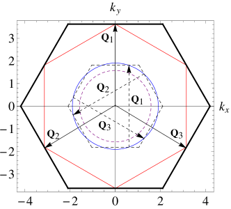
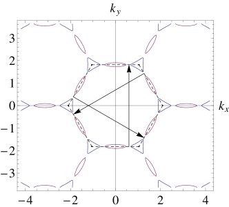
Figure 1: (Color online) The non-interacting Fermi surfaces of spin-up and spin-down electrons (top) at $1/2$ magnetization and the reconstructed fermi surface of spin-down electrons at $y_{\downarrow}/t=0.1$ (bottom). The thick black hexagon is the first Brillouin zone of triangular lattice. The red hexagon is the Fermi surface of the spin-up electron. It is perfectly nested by linear combinations of three wave vectors (the arrows). The dashed hexagon is the first Brillouin zone under the folded scheme. The dashed purple circle is an example of the hot-spot-free Fermi surface of spin-down electrons in the hole doped system.

Next we describe the strong coupling (large-$U$) route and show that $M=\frac{1}{3}M_{\rm sat}$ magnetization plateau ($n_{\uparrow}=2/3,n_{\downarrow}=1/3$), present in the $U/t\to\infty$ limit, survives down to $U_{c1}/t\approx 4.3$, which is significantly lower than the zero-magnetization critical value $U_{120^{\circ}}/t\approx 10$ below which the three-sublattice $120^{\circ}$ magnetic order melts as the system transitions to a quantum spin-liquid state Morita et al. (2002); Sahebsara and Sénéchal (2008); Yang et al. (2010). Quite interestingly, we find that in the interval $U_{c1}\leq U\leq U_{c2}\approx 4.8t$ the UUD state is a half-metal with mobile majority (spin-up) electrons. A closely related question of the evolution of the ground state of the Hubbard model at zero magnetization, as a function of $U/t$, has been actively investigated Morita et al. (2002); Singh (2005); Sahebsara and Sénéchal (2008); Davoudi et al. (2008); Yang et al. (2010), partly because of the potential relevance to intriguing ‘spin-liquid’ organic insulators Motrunich (2005); Lee and Lee (2005); Kanoda and Kato (2011).

Weak-coupling analysis is based on the extended Hubbard model description of electrons on triangular lattice:

$$H = -t\sum_{\langle rr^{\prime}\rangle}(c_{r\sigma}^{\dagger}c_{r^{\prime}\sigma}+{\rm h.c})+U\sum_{r}n_{r\uparrow}n_{r\downarrow}+V\sum_{\langle rr^{\prime}\rangle}n_{r}n_{r^{\prime}}$$ (1)

$$-\sum_{r}\left(\mu+\frac{h\sigma}{2}\right)c_{r\sigma}^{\dagger}c_{r\sigma}.$$

Here $\langle rr^{\prime}\rangle$ labels nearest neighbour bonds, $0<U/t,V/t\ll 1$ are onsite and nearest neighbour repulsive interactions, respectively. For now we set the filling factor at $n=\langle n_{i}\rangle=\langle n_{i\uparrow}+n_{i\downarrow}\rangle=1$.

The Zeeman field $h$, normalized to include the usual $g\mu_{B}$ factor, is tuned to produce $M=\frac{1}{2}M_{\rm sat}$ magnetization so that on average $n_{\uparrow}=3/4$ and $n_{\downarrow}=1/4$ per site. Under this condition the Fermi surface of spin-up electrons, shown in Figure 1, is given by a perfect hexagon whose vertices, located at the M points of the first Brillouin zone (BZ), are van Hove (saddle) points of the dispersion with vanishing Fermi velocity Nandkishore et al. (2012a). These saddle points are the reason for the (logarithmically) diverging density of states as well as singular susceptibility (see below). They are connected by the wave vectors $\mathbf{Q}_{1}=\frac{2\pi}{\sqrt{3}}\hat{y}$ and $\mathbf{Q}_{2,3}=\mp\pi\hat{x}-\frac{\pi}{\sqrt{3}}\hat{y}$ (Fig. 1), which are just halfs of the corresponding reciprocal lattice vectors $\mathbf{G}_{1,2,3}$ Martin and Batista (2008). In addition, parallel faces of the FS are perfectly nested by linear combinations of $\mathbf{Q}$’s. Spin-down FS is nearly circular, as Fig. 1 shows, and does not possess any special features.

The very special role of the wave vectors $\mathbf{Q}_{1,2,3}$ is conveniently quantified by charge susceptibility $\chi_{\sigma}(\mathbf{q})$ of spin-$\sigma$ electrons defined in the standard way as

$$\chi_{\sigma}(\mathbf{q})=\frac{1}{N}\sum_{\mathbf{k}}\frac{n_{\mathbf{k},\sigma}-n_{\mathbf{k}+\mathbf{q},\sigma}}{\epsilon_{\mathbf{k}}-\epsilon_{\mathbf{k}+\mathbf{q}}}.$$ (2)

Here $N$ is the number of sites, $n_{\mathbf{k},\sigma}$ is the occupation number of fermions with spin $\sigma$ and momentum $\mathbf{k}$ and

$$\epsilon_{\mathbf{k}}=-2t\Big{(}\cos k_{x}+2\cos\frac{k_{x}}{2}\cos\frac{\sqrt{3}k_{y}}{2}\Big{)}$$ (3)

is the free-particle dispersion. Straightforward calculation, outlined in sup , shows that susceptibility of spin-up electrons is strongly divergent at $\mathbf{q}=\pm\mathbf{Q}_{a}$, while that of spin-down electrons is finite,

$$\chi_{\uparrow}(\mathbf{Q}_{a}) = -\frac{C_{\uparrow}}{t}\ln^{2}\Big{(}\frac{\Lambda}{q_{0}}\Big{)},~{}C_{\uparrow}=\frac{1}{2\pi^{2}},$$ (4)

$$\chi_{\downarrow}(\mathbf{Q}_{a}) = -\frac{C_{\downarrow}}{t},~{}C_{\downarrow}\approx 0.136.$$ (5)

Here $\Lambda\sim\pi/a$ is the ‘size’ of the BZ ($a$ is the lattice spacing) while $q_{0}\sim 1/L$ is the microscopic cut-off which scales as the inverse linear size of the lattice $L\sim\sqrt{N}a$.

Eq. (4) suggests strong modulation of density at $\mathbf{q}=\pm\mathbf{Q}_{a}$ which motivates the following mean-field ansatz

$$\langle n_{r,\sigma}\rangle=\frac{2+\sigma}{4}+m_{\sigma}\sum_{a=1}^{3}\cos(\mathbf{Q}_{a}\cdot\mathbf{r}),$$ (6)

where index $\sigma$ describes two spin projections, $\sigma=\uparrow=+1$ and $\sigma=\downarrow=-1$, in the usual way. Note that the filling factors $n_{\sigma}=\sum_{\mathbf{r}}\langle n_{r,\sigma}\rangle/N$ are not affected by finite order parameters $m_{\sigma}$, and $n_{\uparrow}=3/4$, while $n_{\downarrow}=1/4$. Ansatz (6) allows us to approximate (1) as

$$H = \sum_{\mathbf{k},\sigma}(\epsilon_{\mathbf{k}}-\mu_{\sigma})c^{+}_{\mathbf{k}\sigma}c_{\mathbf{k}\sigma}+\frac{1}{2}\sum_{\mathbf{k},\sigma,a}y_{\sigma}(c^{+}_{\mathbf{k}\sigma}c_{\mathbf{k}+\mathbf{Q}_{a}\sigma}+{\rm h.c.})$$ (8)

$$+3NV(m_{\uparrow}+m_{\downarrow})^{2}-3NUm_{\uparrow}m_{\downarrow},$$

$$y_{\sigma}=Um_{-\sigma}-2V(m_{\uparrow}+m_{\downarrow}),$$

The amplitudes of density modulation of spin-$\sigma$ electrons are determined self-consistently

$$m_{\sigma} = \frac{1}{3N}\sum_{\mathbf{r},a}\cos(\mathbf{Q}_{a}\cdot\mathbf{r})\langle n_{\mathbf{r},\sigma}\rangle$$ (9)

$$=\frac{y_{\sigma}}{3N}\sum_{\mathbf{k},a}\frac{n_{\mathbf{k},\sigma}-n_{\mathbf{k}+\mathbf{Q}_{a},\sigma}}{\tilde{\epsilon}_{\mathbf{k}}-\tilde{\epsilon}_{\mathbf{k}+\mathbf{Q}_{a}}}=y_{\sigma}\chi_{\sigma}(\mathbf{Q}_{a}),$$

where dispersion $\tilde{\epsilon}_{\mathbf{k}}$ is determined by the mean-field Hamiltonian (8). We find $m_{\downarrow}=C_{\downarrow}(V-U/2)m_{\uparrow}/t$, which means $|m_{\downarrow}|\ll|m_{\uparrow}|$, and

$$\frac{C_{\uparrow}}{t}\ln^{2}\Big{(}\frac{\Lambda}{q_{\uparrow}}\Big{)}=\Big{(}V+\frac{C_{\downarrow}}{t}(V-\frac{U}{2})^{2}\Big{)}^{-1}.$$ (10)

The main effect of interaction $y_{\uparrow}$ in (8) is to provide an infra-red cut-off $q_{\uparrow}\sim|y_{\uparrow}/t|^{1/2}$ in the susceptibility (4) of spin-up electrons at the van Hove points. This leads to the final result

$$m_{\uparrow} = -\frac{\Lambda^{2}t}{V+\frac{C_{\downarrow}}{t}(V-U/2)^{2}}$$ (11)

$$\times\exp\left(-\sqrt{\frac{4t}{C_{\uparrow}[V+\frac{C_{\downarrow}}{t}(V-U/2)^{2}]}}\right).$$

Non-analytic dependence of $m$ on interaction amplitudes $U,V$ is determined by van Hove points. The sign of $m_{\uparrow}$ is chosen such that the FS of spin-up electrons is gapped for all momenta. We checked that the opposite sign leads to a quadratic touching of the top two bands at $\Gamma$ point and results in a state of higher energy sup .

Equations (6) and (11) show that the ground state is a superposition of commensurate charge-density and collinear spin-density waves. This is a four-sublattice state: observe that $\sum_{a=1}^{3}\cos(\mathbf{Q}_{a}\cdot\mathbf{r})$ takes values $3,-1,-1,-1$ on the sites of triangular lattice $\mathbf{r}=(x,y)=d_{1}\mathbf{a}_{1}+d_{2}\mathbf{a}_{2}$, where $\mathbf{a}_{1}=(1,0)$ and $\mathbf{a}_{2}=(1/2,\sqrt{3}/2)$ are elementary lattice vectors and $d_{1,2}$ are integers. We stress that the perfectly nested FS of spin-up electrons is crucial for the spin-up electrons to be gapped at arbitrary weak interaction.

Note that in the absence of direct density-density interaction, when $V=0$, the order parameter scales as $m\sim\exp\left(-{\rm const}/U\right)$. The density wave of spin-up electrons in this case is driven by the effective interaction $\propto\chi_{\downarrow}U^{2}$, which is mediated by spin-down electrons, since the onsite repulsion $U$ only couples electrons of opposite spins. A small finite $V\geq U^{2}/t$, see (11), changes this scaling to a much stronger dependence $m\sim\exp\left(-{\rm const}/\sqrt{V}\right)$.

The band structure of spin-down electrons is also modified as (8) shows. For finite $y_{\downarrow}$, while the spin-down electrons remain gapless, the ‘hot spots’ on the spin-down FS (which are the points connected by $\mathbf{Q}_{a}$) are gapped and the FS is reconstructed as shown in Figure 1. By reducing the density of spin-down electrons $n_{\downarrow}$ below $1/4$, while maintaining that of spin-up ones at the perfect nesting condition $n_{\uparrow}=3/4$, one can reduce the spin-down FS below the critical volume to make it fit inside the reduced Brillouin zone (dashed hexagon in Fig. 1), which is 4 times smaller than the original one, and the hot spots disappear altogether. We find that this happens for $n_{\rm cr}<0.976$ (Figure 1), i.e. $n_{{\rm cr}\downarrow}<0.226$. Under this condition, and for weak interactions $U,V\ll t$, the FS of spin-down electrons is not affected by the reconstruction of the FS of spin-up electrons at all. In either case, the result is a half-metal where all conducting electrons have spin opposite to the direction of the external field.

Similar half-metallic state can be realized on other lattices. For example, consider the same Hamiltonian (1) on the square lattice with filling factor $n\neq 1$. A proper field $h$ can be applied such that the FS of the spin-up (if total density $n<1$) or the spin-down (if $n>1$) electrons is perfectly nested. Clearly this FS is a square with vertices at $(\pm\pi,0)$ and $(0,\pm\pi)$ points. The system then develops density wave order at wave vector $\mathbf{Q}=(\pi,\pi)$. The ordered state is generically half-metallic. Note also that in this case the FS of conduction electrons experiences no reconstruction due to the absence of hot spots.

Strong coupling limit. We now turn to the question of $M=\frac{1}{3}M_{\rm sat}$ plateau which exists in the opposite limit of strong interactions, $U\gg t$. As should be clear from the previous discussion, in the current situation filling factors of spin-up (down) electrons $2/3(1/3)$ do not correspond to perfectly nested FS. In order to make connection with the insulating magnetization plateau phase of the Heisenberg spin model we set $V=0$, keep total density at one electron per site $n=1$ and introduce the following mean-field ansatz:

$$\langle n_{\mathbf{r}\sigma}\rangle=\frac{1}{2}+\frac{\sigma}{6}-2\eta_{\sigma}\cos(\mathbf{Q}\cdot\mathbf{r})$$ (12)

where $\mathbf{Q}=\frac{4\pi}{3}\hat{x}$ describes the UUD pattern. (Note that $\cos(\mathbf{Q}\cdot\mathbf{r})$ takes values $1,-1/2,-1/2$ on the triangular lattice.) Parameters $\eta_{\sigma}$ of the state are determined self-consistently by the equations similar to (9). Solving them numerically we find discontinuous jump of $\eta_{\sigma}$ from zero to finite values when $U\geq 4.30t$ for a range of $h$. We also find that $\eta_{\uparrow}$ and $\eta_{\downarrow}$ are in general different so that the system displays a co-existence of the spin-density and charge-density wave orders sup . Interestingly, it is now the spin-down electrons that are gapped while the spin-up electrons remain gapless around the Fermi energy, see Figure 2. Spin-down electrons fill completely the lowest of the three bands $\omega_{\downarrow}(\mathbf{k})$ in the folded Brillouin zone, while the spin-up ones fill the two lowest bands $\omega_{\uparrow}(\mathbf{k})$. For even stronger interaction $U>4.80t$, the two upper spin-up bands also get separated by a gap which turns the half-metal state into an insulator with collinear UUD pattern of local magnetization.

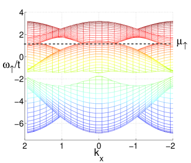
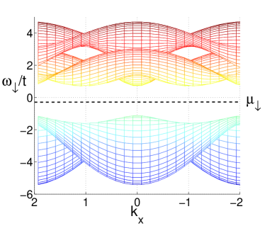
Figure 2: (Color online) The spin-up (top) and spin-down (bottom) bands of the half-metal state at $1/3$ magnetization at $U=4.60t$. In order to give an idea of dispersion along the $k_{y}$ axis as well, the graph shows projections of two-dimensional bands onto $k_{x}$ axis for 30 different discrete $k_{y}$ values. The Fermi energies $\mu_{\sigma}=\mu+\sigma(h/2+U/6)$ are shown as black-dash lines.

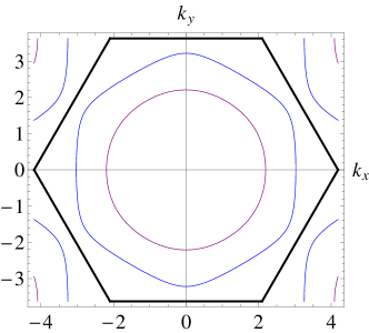
Figure 3: The Fermi surfaces of spin-up (blue) and spin-down (purple) electrons at $M=\frac{1}{3}~{}M_{\mathrm{sat}}$ for $\eta_{\sigma}=0$.

To estimate how competitive the found half-metal state is we compared its energy with the uniformly magnetized transverse spin-density wave state, i.e. “cone” state in magnetic language. This state is characterized by the two order parameters, longitudinal $\langle S^{z}_{\mathbf{r}}\rangle=M$ and transverse $\langle S^{+}_{\mathbf{q}}\rangle=m_{0}e^{i\mathbf{q}\cdot\mathbf{r}}$ magnetizations Krishnamurthy et al. (1990); Jayaprakash et al. (1991), where the ordering wave vector $\mathbf{q}$ is incommensurate in general. Comparing their mean-field energies, we determined that the half-metal state has a lower energy for $4.45t\leq U\leq 4.80t$ sup . The resulting mean-field phase diagram is shown in Figure 3. Note that both half-metal and insulator phases are magnetization plateau states with $M=\frac{1}{3}M_{\rm sat}$.

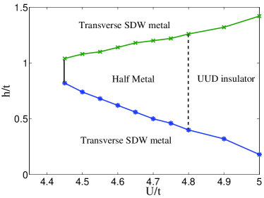
Figure 3: (Color online) The mean-field phase boundaries of the half-metal and insulating states at $M=1/3~{}M_{\rm sat}$ on triangular lattice. Solid (dashed) lines denote first (second) order transitions.

Discussion: we described two general ways to induce half-metal states through a combination of electronic interactions and a finite Zeeman field. Our work provides new avenue to half-metallic states which have potential applications in future spin-dependent electronics. Despite our focus on the Hubbard-Heisenberg model on the triangular lattice, both of the proposed mechanisms can be easily generalized to other lattice geometries. It is important to note that in our proposal the Zeeman field sets direction of the spin polarization of conducting electrons in the half-metal state. This convenient feature makes it different from the recently discussed half-metal SDW state at zero magnetization Nandkishore et al. (2012a) where spin-rotational symmetry breaks spontaneously, resulting in a random selection of the spin polarization axis in the spin space.

Our proposal can also be realized in Kondo lattice systems where the Zeeman field is provided by exchange couplings between the itinerant electrons and ferromagnetically ordered local moments, see e.g. Martin and Batista (2008), as well as in cold atom systems Partridge et al. (2006); Zwierlein et al. (2006) where it may be easier to achieve the required spin population imbalance.

Magnetic field control of the half-metallic phase may be useful for creating switchable interfaces between half-metal and noncentrosymmetric superconductor which have been argued to support Majorana bound states Duckheim and Brouwer (2011).

It is worth noting close physical similarity between our proposal and the previously proposed one-dimensional ‘Coulomb drag’ setup Pustilnik et al. (2006) where role of the lattice is played by the electrons in an active wire interactions with which gap out one of the spin projections in the passive wire.

Several interesting theoretical questions can be asked regarding the half-metal state. First of all, the metal-insulator transition between a half-metal and a Mott insulator, found here at $U/t\approx 4.8$, represents Mott transition which is not affected by (gapped) spin fluctuations. Understanding it in details may lead one to a better characterization of the general Mott transition. Half metal states are adjacent to many other interesting quantum phases. For example, it was demonstrated Nandkishore et al. (2012b) that $d+id$ chiral superconducting state is the ground state at $3/2$ ($5/8$) filling on triangular (honeycomb) lattice for weak interaction. If we dope the system with holes while keeping the FS of spin-up electrons perfectly nested by a Zeeman field, the system will eventually become a half-metal. Understanding how quantum phase transition(s) between these different phases happen is an interesting question left for future studies.

We would like to thank A. V. Chubukov, L. I. Glazman, M. J. P. Gingras, E. G. Mishchenko, M. E. Raikh and O. V. Tchernyshyov for useful discussions. This work was initiated at the Max-Planck Institute for the Physics of Complex Systems during the activities of the Advanced Study Group Program on “Unconventional Magnetism in High Field”, which we would like to thank for hospitality. The work is supported by NSF through Grant No. DMR-0808842 (O.A.S.) and by NSERC of Canada (Z.H.).

Supplementary Material for ”Half-metallic magnetization plateaux” by Zhihao Hao and Oleg A. Starykh

Appendix A Susceptibility

Susceptibility $\chi_{\sigma}(\mathbf{Q}_{a})$ ($a=1,2,3$) of free electrons is given by

$$\chi_{\sigma}(\mathbf{Q}_{a})=\frac{1}{A}\int d^{2}k\frac{n_{\mathbf{k},\sigma}-n_{\mathbf{k}+\mathbf{Q}_{a},\sigma}}{\epsilon_{\mathbf{k}}-\epsilon_{\mathbf{k}+\mathbf{Q}_{a}}}$$ (1)

where the integration is restricted in the first Brillouin zone of area $A=8\pi^{2}/\sqrt{3}$. $\epsilon_{\mathbf{k}}=-2\left(\cos k_{x}+2\cos\frac{k_{x}}{2}\cos\frac{\sqrt{3}k_{y}}{2}\right)$ is the dispersion of the non-interacting fermion. Due to six-fold rotational symmetry, $\chi_{\sigma}(\mathbf{Q}_{a})$ is independent of $a$. We consider $\sigma=\uparrow$ and $a=1$. The particle ($n_{\mathbf{k}}=1$) and hole ($n_{\mathbf{k}}=0$) states contribute equally to $\chi$. In addition, the integrand is invariant under separate operations $k_{x}\to-k_{x}$ and $k_{y}\to-k_{y}$. Taking advantage of these symmetries, we compute the leading singular contribution to $\chi$ by writing $\mathbf{k}=(\pi,\pi/\sqrt{3})+\mathbf{q}$ and considering small $q$ limit:

$$\chi_{\uparrow}(\mathbf{Q}_{1}) \approx-\frac{8}{2\sqrt{3}At}\int_{-\Lambda}^{-q_{0}}dq_{x}\int_{-\Lambda}^{\sqrt{3}q_{x}}dq_{y}\frac{1}{q_{x}q_{y}}$$ (2)

$$\approx-\frac{1}{2\pi^{2}t}\ln^{2}\left(\frac{\Lambda}{q_{0}}\right).$$

For $\sigma=\downarrow$, $\chi_{\downarrow}$ is computed numerically:

$$\chi_{\downarrow}(\mathbf{Q}_{1})\approx-\frac{0.136}{t}.$$ (3)

Appendix B Half-metal state at weak coupling

We consider only spin-up fermions on triangular lattice at $3/4$ filling. The following Hamiltonian is studied:

$$H=\sum_{\mathbf{k}}\left((\epsilon_{\mathbf{k}}-\mu)c_{\mathbf{k}\uparrow}^{\dagger}c_{\mathbf{k}\uparrow}+\frac{y}{2}\sum_{a=1}^{3}(c_{\mathbf{k}\uparrow}^{\dagger}c_{\mathbf{k}+\mathbf{Q}_{q}\uparrow}+{\rm h.c})\right).$$ (4)

The Hamiltonian can be diagonalized and we obtain four bands in the folded zone scheme. In the limit of $y\to 0$, three of the four bands become $\epsilon_{\mathbf{k}+\mathbf{Q}_{a}}$ ($a=1,2,3$). These bands touch at three straight lines through the $\Gamma$ point (Fig. 1). The spectrum at $\mathbf{k}=0$ is $-8$, $-y$, $-y$ and $2y$. For $y>0$, the lower three bands are $-8$, $-y$ and $-y$. The Fermi surface is fully gapped. For $y<0$, the Fermi surface become a point at $\mathbf{k}=0$.

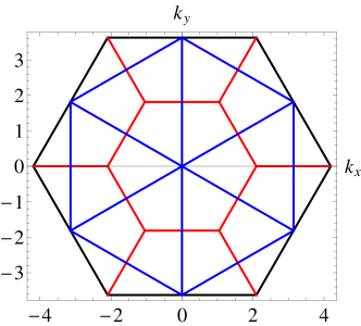
Figure 1: The Fermi surface at $y_{\uparrow}=0$ (the blue lines) under the folded zone scheme. The folded zone (the red hexagons) is four times smaller than the first Brillouin zone of the triangular lattice (the black hexagon).

We define the energy of the Fermi sea to be $E(y)$. At small $|y|$, the band structures of $y>0$ and $y<0$ are only significantly different around the $\Gamma$ point. $E(y)$ for positive $y$ is lowered by order $|y|$ in an area proportional to $|y|$ around $\mathbf{k}=0$ since the energies at the van Hove point are functions of $\mathbf{k}^{2}$ for small $k$. $\delta E(|y|)\equiv E(-|y|)-E(|y|)$ can then be estimated as proportional to $\chi_{\uparrow}(|y|)y^{2}\sim\ln^{2}(|y|^{1/2})y^{2}$, as shown by the red line in Fig. 2. The blue points are obtained by numerically calculating $\delta E(|y|)$ as a function of momentum $\mathbf{k}$ and summing over fine mesh of $k$-points in the Brillouin zone.

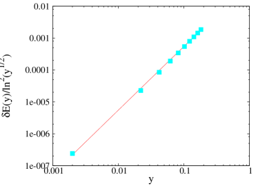
Figure 2: $\delta E(y)/\ln^{2}(y^{1/2})$ (blue squares) as a function of $y$ fitted by function $0.055y^{2}$ (the red line).

Appendix C $M=M_{{\rm sat}}/3$  half-metal state

We use the following mean-field ansatz:

$$\langle n_{\mathbf{r}\sigma}\rangle=\frac{1}{2}+\frac{\sigma}{6}-2\eta_{\sigma}\cos(\mathbf{Q}\cdot\mathbf{r}).$$

The mean-field Hamiltonian can be written as:

$$H= -\sum_{\langle\mathbf{r}_{1}\mathbf{r}_{2}\rangle}(c_{\mathbf{r}_{1}\sigma}^{\dagger}c_{\mathbf{r}_{2}\sigma}+h.c)-\sum_{\mathbf{r}}\left(\mu+\frac{h\sigma}{2}+\frac{U\sigma}{6}\right)c_{\mathbf{r}\sigma}^{\dagger}c_{\mathbf{r}\sigma}$$ (5)

$$-2U\sum_{\mathbf{r}}\eta_{-\sigma}\cos(\mathbf{Q}_{a}\cdot\mathbf{r})c_{\mathbf{r}\sigma}^{\dagger}c_{\mathbf{r}\sigma}-2NU\eta_{\uparrow}\eta_{\downarrow}$$

$$+\frac{5UN}{18}.$$

The self-consistent equations read:

$$\eta_{\sigma} = -\frac{1}{N}\sum_{\mathbf{r}}\cos(\mathbf{Q}_{a}\cdot\mathbf{r})\langle c_{\mathbf{r}\sigma}^{\dagger}c_{\mathbf{r}\sigma}\rangle,$$ (6a)

$$1 = \frac{1}{N}\sum_{\mathbf{r}}c^{\dagger}_{\mathbf{r}\sigma}c_{\mathbf{r}\sigma}.$$ (6b)

These equations are solved numerically. $\eta_{\sigma}$ become finite for $U>4.3t$ (Fig. 4).

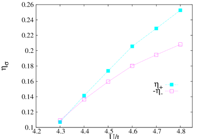
Figure 4: $\eta_{\sigma}$ as a function of $U$.

We compare the energy of the half-metal state with a second mean-field ansatz: a spiral spin-density wave with a uniform magnetization. We use the following notation for order parameters: $\langle S^{z}_{\mathbf{r}}\rangle=M$ and $\langle S^{+}_{\mathbf{Q}}\rangle=m_{0}e^{i\mathbf{Q}\cdot\mathbf{r}}$

Define the two component spinor as $\psi_{\mathbf{k}}=(c_{\mathbf{k}+\mathbf{Q}\uparrow},c_{\mathbf{k}\downarrow})^{T}$, the Hamiltonian can be written as:

$$H = \sum_{\mathbf{k}}\psi^{\dagger}_{\mathbf{k}}\Big{[}(\epsilon_{\mathbf{k}+\mathbf{Q}}+\epsilon_{\mathbf{k}}-\mu)I+(\epsilon_{\mathbf{k}+\mathbf{Q}}-\epsilon_{\mathbf{k}}-\frac{h}{2}-UM)\sigma_{z}$$ (7)

$$-Um_{0}\sigma_{x}\Big{]}\psi_{\mathbf{k}}+NUM^{2}+NUm_{0}^{2}.$$

where $\epsilon_{\mathbf{k}}=-2t(\cos(k_{x})+2\cos(k_{x}/2)\cos(\sqrt{3}k_{y}/2))$. The spectrum can be solved:

$$\omega_{\pm}= \epsilon_{\mathbf{k}+\mathbf{Q}}+\epsilon_{\mathbf{k}}\pm\sqrt{(\epsilon_{\mathbf{k}+\mathbf{Q}}-\epsilon_{\mathbf{k}}-\frac{h}{2}-UM)^{2}+U^{2}m_{0}^{2}}$$ (8)

$$\equiv \epsilon_{\mathbf{k}+\mathbf{Q}}+\epsilon_{\mathbf{k}}\pm g_{\mathbf{k}}.$$

The self consistent equations read:

$$M= \frac{1}{2N}\sum_{\mathbf{k}}\frac{\epsilon_{\mathbf{k}+\mathbf{Q}}-\epsilon_{\mathbf{k}}-\frac{h}{2}-UM}{g_{\mathbf{k}}}\sum_{\sigma}\sigma\Theta(\mu-\omega_{\sigma}),$$ (9)

$$m_{0}= \frac{1}{2N}\sum_{\mathbf{k}}\frac{Um_{0}}{g_{\mathbf{k}}}\sum_{\sigma}\sigma\Theta(\mu-\omega_{\sigma}),$$

$$1= \frac{1}{N}\sum_{\sigma}\Theta(\mu-\omega_{\sigma}).$$

Here $\Theta(x)=1$ for $x>0$ and $\Theta(x)=0$ for $x<0$.

For fixed $U$ and $h$, we solve the self-consistency equations numerically for different $\mathbf{Q}$’s. Focusing on $\mathbf{Q}=(Q_{x},0)$, we find the $\mathbf{Q}^{\mathrm{(min)}}$ with lowest mean-field energy. $\mathbf{Q}^{(min)}$ is incommensurate in general (Fig. 5). We scan over the two dimensional phase space $\mathbf{Q}$ for some $U$’s and confirm that the lowest mean-field energy state is indeed on the $Q_{y}=0$ axis.

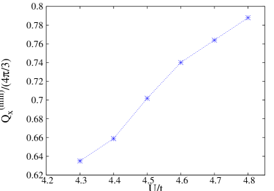
Figure 5: $Q_{x}^{\mathrm{(min)}}/(4\pi/3)$ as a function of $U$.

Comparing the mean-field energy of the two states, the half-metal state has lower energy for $U>4.45t$ for ranges of $h$. For $U>4.8t$, the half-metal state becomes a band insulator.

References

- Kodama et al. (2002) K. Kodama, M. Takigawa, M. Horvatic, C. Berthier, H. Kageyama, Y. Ueda, S. Miyahara, F. Becca, and F. Mila, Science 298, 395 (2002).
- Kikuchi et al. (2005) H. Kikuchi, Y. Fujii, M. Chiba, S. Mitsudo, T. Idehara, T. Tonegawa, K. Okamoto, T. Sakai, T. Kuwai, and H. Ohta, Phys. Rev. Lett. 94, 227201 (2005).
- Ueda et al. (2005) H. Ueda, H. A. Katori, H. Mitamura, T. Goto, and H. Takagi, Phys. Rev. Lett. 94, 047202 (2005).
- Fortune et al. (2009) N. A. Fortune, S. T. Hannahs, Y. Yoshida, T. E. Sherline, T. Ono, H. Tanaka, and Y. Takano, Phys. Rev. Lett. 102, 257201 (2009).
- Nema et al. (2009) H. Nema, A. Yamaguchi, T. Hayakawa, and H. Ishimoto, Phys. Rev. Lett. 102, 075301 (2009).
- Kawamura and Miyashita (1985) H. Kawamura and S. Miyashita, Journal of the Physical Society of Japan 54, 4530 (1985).
- Chubukov and Golosov (1991) A. V. Chubukov and D. I. Golosov, Journal of Physics: Condensed Matter 3, 69 (1991).
- Alicea et al. (2009) J. Alicea, A. V. Chubukov, and O. A. Starykh, Phys. Rev. Lett. 102, 137201 (2009).
- Griset et al. (2011) C. Griset, S. Head, J. Alicea, and O. A. Starykh, Phys. Rev. B 84, 245108 (2011).
- de Groot et al. (1983) R. A. de Groot, F. M. Mueller, P. G. v. Engen, and K. H. J. Buschow, Phys. Rev. Lett. 50, 2024 (1983).
- Katsnelson et al. (2008) M. I. Katsnelson, V. Y. Irkhin, L. Chioncel, A. I. Lichtenstein, and R. A. de Groot, Rev. Mod. Phys. 80, 315 (2008).
- Martin and Batista (2008) I. Martin and C. D. Batista, Phys. Rev. Lett. 101, 156402 (2008).
- Nandkishore et al. (2012a) R. Nandkishore, G.-W. Chern, and A. V. Chubukov, Phys. Rev. Lett. 108, 227204 (2012a).
- Chern et al. (2012) G.-W. Chern, R. M. Fernandes, R. Nandkishore, and A. V. Chubukov, ArXiv e-prints (2012), eprint 1203.5776.
- Chern and Batista (2012) G.-W. Chern and C. D. Batista, ArXiv e-prints (2012), eprint 1204.5737.
- Metlitski and Sachdev (2010) M. A. Metlitski and S. Sachdev, Phys. Rev. B 82, 075128 (2010).
- Morita et al. (2002) H. Morita, S. Watanabe, and M. Imada, Journal of the Physical Society of Japan 71, 2109 (2002).
- Sahebsara and Sénéchal (2008) P. Sahebsara and D. Sénéchal, Phys. Rev. Lett. 100, 136402 (2008).
- Yang et al. (2010) H.-Y. Yang, A. M. Läuchli, F. Mila, and K. P. Schmidt, Phys. Rev. Lett. 105, 267204 (2010).
- Singh (2005) A. Singh, Phys. Rev. B 71, 214406 (2005).
- Davoudi et al. (2008) B. Davoudi, S. R. Hassan, and A.-M. S. Tremblay, Phys. Rev. B 77, 214408 (2008).
- Motrunich (2005) O. I. Motrunich, Phys. Rev. B 72, 045105 (2005).
- Lee and Lee (2005) S.-S. Lee and P. A. Lee, Phys. Rev. Lett. 95, 036403 (2005).
- Kanoda and Kato (2011) K. Kanoda and R. Kato, Annual Review of Condensed Matter Physics 2, 167 (2011).
- (25) See Supplementary Material for more details.
- Krishnamurthy et al. (1990) H. R. Krishnamurthy, C. Jayaprakash, S. Sarker, and W. Wenzel, Phys. Rev. Lett. 64, 950 (1990).
- Jayaprakash et al. (1991) C. Jayaprakash, H. R. Krishnamurthy, S. Sarker, and W. Wenzel, Europhysics Letters 15, 625 (1991).
- Partridge et al. (2006) G. B. Partridge, W. Li, R. I. Kamar, Y.-A. Liao, and R. G. Hulet, Science 311, 503 (2006).
- Zwierlein et al. (2006) M. W. Zwierlein, A. Schirotzek, C. H. Schunck, and W. Ketterle, Science 311, 492 (2006).
- Duckheim and Brouwer (2011) M. Duckheim and P. W. Brouwer, Phys. Rev. B 83, 054513 (2011).
- Pustilnik et al. (2006) M. Pustilnik, E. G. Mishchenko, and O. A. Starykh, Phys. Rev. Lett. 97, 246803 (2006).
- Nandkishore et al. (2012b) R. Nandkishore, L. S. Levitov, and A. V. Chubukov, Nat Phys 8, 158 (2012b).