Spherical coupled-cluster theory for open-shell nuclei

Abstract

Background

A microscopic description of nuclei is important to understand the nuclear shell-model from fundamental principles. This is difficult to achieve for more than the lightest nuclei without an effective approximation scheme.

Purpose

Define and evaluate an approximation scheme that can be used to study nuclei that are described as two particles attached to a closed (sub-)shell nucleus.

Methods

The equation-of-motion coupled-cluster formalism has been used to obtain ground and excited state energies. This method is based on the diagonalization of a non-Hermitian matrix obtained from a similarity transformation of the many-body nuclear Hamiltonian. A chiral interaction at the next-to-next-to-next-to leading order (N³LO) using a cutoff at $500$ MeV was used.

Results

The ground state energies of ⁶Li and ⁶He were in good agreement with a no-core shell-model calculation using the same interaction. Several excited states were also produced with overall good agreement. Only the $J^{\pi}=3^{+}$ excited state in ⁶Li showed a sizable deviation. The ground state energies of ¹⁸O, ¹⁸F and ¹⁸Ne were converged, but underbound compared to experiment. Moreover, the calculated spectra were converged and comparable to both experiment and shell-model studies in this region. Some excited states in ¹⁸O were high or missing in the spectrum. It was also shown that the wave function for both ground and excited states separates into an intrinsic part and a Gaussian for the center-of-mass coordinate. Spurious center-of-mass excitations are clearly identified.

Conclusions

Results are converged with respect to the size of the model space and the method can be used to describe nuclear states with simple structure. Especially the ground state energies were very close to what has been achieved by exact diagonalization. To obtain a closer match with experimental data, effects of three-nucleon forces, the scattering continuum as well as additional configurations in the coupled-cluster approximations, are necessary.

I Introduction

In the past decade, the computing resources made available for scientific research has grown several orders of magnitude. This trend will continue during this decade, culminating in exascale computing facilities. This will promote new insights in every discipline as new problems can be solved and old problems can be solved faster and to a higher precision.

In nuclear physics, one important goal is a predictive theory, where nuclear observables can be calculated from first principles. But even with the next generation of supercomputers, a virtually exact solution to the nuclear many-body problem is possible only for light nuclei (see Leidemann and Orlandini (2013) for a recent review on many-body methods). Using a finite basis expansion, a full diagonalization can currently be performed for nuclei in the $p$-shell region Navrátil et al. (2009). This might be extended to light $sd$-shell nuclei within the next couple of years with access to sufficient computing resources. For ab initio access to larger nuclei, the problem has to be approached differently Dickhoff and Barbieri (2004); Hagen et al. (2007a); Roth and Navrátil (2007); Tsukiyama et al. (2011); Somà et al. (2013).

In coupled-cluster theory, a series of controlled approximations are performed to generate a similarity transformation of the nuclear Hamiltonian. At a given level of approximation, efficient formulas exist to evaluate the ground state energy of a closed (sub-)shell reference nucleus. The similarity-transformed Hamiltonian is then diagonalized to calculate excited states and states of nuclei with one or more valence nucleons. This defines the equation-of-motion coupled-cluster (EOM-CC) framework (see Bartlett and Musiał (2007) for a recent review and Shavitt and Bartlett (2009) for a textbook presentation). Recently, this method was applied to the oxygen Hagen et al. (2012a) and the calcium Hagen et al. (2012b) isotopic chains, as well as ⁵⁶Ni Binder et al. (2013), extending the reach of ab initio methods in the medium mass region. Further calculations in the nickel and tin regions are also planned.

In this work, I will refine the EOM-CC method for two valence nucleons attached to a closed (sub-)shell reference (2PA-EOM-CC). The general theory was presented in Jansen et al. (2011), where calculations were limited to small model spaces. The working equations are now completely reworked in a spherical formalism. Since the Hamiltonian is invariant under rotation, this formalism enables us to do calculations in significantly larger model spaces. All relevant equations of spherical formalism are explicitly included here for future reference. The method, in the form presented here, has already been successfully applied to several nuclei Hagen et al. (2012a, b); Ekström et al. (2013); Lepailleur et al. (2013), but the formalism has not been presented.

A brief overview of general coupled-cluster theory and the equation-of-motion extensions is given in Sec. II. In Sec. III I derive the working equations for 2PA-EOM-CC and discuss numerical results for selected $p$- and $sd$-shell nuclei in Sec. IV. As a proper treatment of three body forces and continuum degrees of freedom is beyond the scope of this article, the focus will be on convergence, rather than comparison to experiment. Finally, in Sec. V I present conclusions and discuss the road ahead. All angular momentum transformations used in this work are defined in the appendix.

II Coupled-cluster theory

In this section the Hamiltonian that enters the coupled-cluster calculations is defined. I have also included a brief review of single reference coupled cluster-theory together with the equation-of-motion (EOM-CC) extensions. In this framework, a diagonalization in a truncated vector space yields excited states, where also nuclei with different particle numbers can be approached by choosing an appropriate basis. The presentation is kept short and is focused on the aspects important for deriving the spherical version of the 2PA-EOM-CCSD method presented in Sec. III.

All calculations are done using the intrinsic Hamiltonian

$$\mathrm{\hat{H}}=\left(1-\frac{1}{A^{*}}\right)\sum_{i=1}^{A}\frac{p_{i}^{2}}{2m}+\left[\sum_{i<j=1}^{A}\mathrm{\hat{v}}_{ij}-\frac{\vec{p}_{i}\cdot\vec{p}_{j}}{mA^{*}}\right]\ .$$ (1)

Here $A$ is the number of nucleons in the reference state, $A^{*}=A+2$ is the mass number of the target nucleus, and $\mathrm{\hat{v}}_{ij}$ is the nucleon-nucleon interaction. Only two-body interactions are included at present. In the second quantization, the Hamiltonian can be written as

$$\mathrm{\hat{H}}=\sum_{pq}\varepsilon^{p}_{q}a^{\dagger}_{p}a_{q}+\frac{1}{4}\sum_{pqrs}\langle pq||rs\rangle a^{\dagger}_{p}a^{\dagger}_{q}a_{s}a_{r}\ .$$ (2)

The term $\langle pq||rs\rangle$ is a shorthand for the matrix elements (integrals) of the two-body part of the Hamiltonian of Eq. (1), $p,q,r$ and $s$ represent various single-particle states while $\varepsilon^{p}_{q}$ stands for the matrix elements of the one-body operator in Eq. (1). Finally, second quantized operators like $a^{\dagger}_{q}$ and $a_{p}$ create and annihilate a nucleon in the states $q$ and $p$, respectively. These operators fulfill the canonical anti-commutation relations.

II.1 Single-reference coupled-cluster theory

In single-reference coupled-cluster theory, the many-body ground-state $|\Psi_{0}\rangle$ is given by the exponential ansatz,

$$|\Psi_{0}\rangle=\exp{(\mathrm{\hat{T}})}|\Phi_{0}\rangle\ .$$ (3)

Here, $|\Phi_{0}\rangle$ is the reference Slater determinant, where all states below the Fermi level are occupied and $\mathrm{\hat{T}}$ is the cluster operator that generates correlations. The operator $\mathrm{\hat{T}}$ is expanded as a linear combination of particle-hole excitation operators

$$\mathrm{\hat{T}}=\mathrm{\hat{T}}_{1}+\mathrm{\hat{T}}_{2}+\ldots+\mathrm{\hat{T}}_{A}\,$$ (4)

where $\mathrm{\hat{T}}_{n}$ is the $n$-particle-$n$-hole($n$p-$n$h) excitation operator

$$\mathrm{\hat{T}}_{n}=\left(\frac{1}{n!}\right)^{2}\sum_{a_{\nu}i_{\nu}}t_{i_{1}\ldots i_{n}}^{a_{1}\ldots a_{n}}a^{\dagger}_{a_{1}}\dots a^{\dagger}_{a_{n}}a_{i_{n}}\dots a_{i_{1}}\ .$$ (5)

Throughout this work the indices $ijk\ldots$ denote states below the Fermi level (holes), while the indices $abc\ldots$ denote states above the Fermi level (particles). For an unspecified state, the indices $pqr\ldots$ are used. The amplitudes $t_{i_{1}\ldots i_{n}}^{a_{1}\ldots a_{n}}$ will be determined by solving the coupled-cluster equations. In the singles and doubles approximation the cluster operator is truncated as

$$\mathrm{\hat{T}}\approx\mathrm{\hat{T}}_{\rm CCSD}\equiv\mathrm{\hat{T}}_{1}+\mathrm{\hat{T}}_{2}\ ,$$ (6)

which defines the coupled-cluster approach with singles and doubles excitations, the so-called CCSD approximation. The unknown amplitudes result from the solution of the non-linear CCSD equations given by

$$\langle\Phi_{i}^{a}|\mathrm{\bar{H}}|\Phi_{0}\rangle = 0,$$

$$\langle\Phi_{ij}^{ab}|\mathrm{\bar{H}}|\Phi_{0}\rangle = 0\ .$$ (7)

The term

$$\mathrm{\bar{H}}=\exp{(-\mathrm{\hat{T}})}\mathrm{\hat{H}}_{N}\exp{(\mathrm{\hat{T}})}=\left(\mathrm{\hat{H}}_{N}\exp{(\mathrm{\hat{T}})}\right)_{C},$$ (8)

is called the similarity-transform of the normal-ordered Hamiltonian. In this formulation, the state $|\Phi_{ij\dots}^{ab\dots}\rangle$ is a Slater determinant that differs from the reference $|\Phi_{0}\rangle$ by holes in the orbitals $ij\dots$ and by particles in the orbitals $ab\dots$. The subscript $C$ indicates that only connected diagrams enter, while the normal-ordered Hamiltonian is defined as

$$\mathrm{\hat{H}}_{N}=\mathrm{\hat{F}}+\mathrm{\hat{V}}_{N}-E_{0},$$ (9)

The operator $\mathrm{\hat{F}}$ is the onebody part of the normal-ordered Hamiltonian defined as

$$\mathrm{\hat{F}}=\sum_{pq}f_{q}^{p}\left\{a^{\dagger}_{p}a_{q}\right\},$$ (10)

where

$$f^{p}_{q}=\epsilon_{q}^{p}+\sum_{i}\langle pi||qi\rangle.$$ (11)

Here $\epsilon_{q}^{p}$ and $\langle pi||qi\rangle$ are the matrix elements of the Hamiltonian in Eq. (2). The sum is over all single particle indices, $i$, below the Fermi energy. The operator $\mathrm{\hat{V}}_{N}$ is the twobody part of the normal-ordered Hamiltonian, while $E_{0}$ denotes the vacuum expectation value with respect to the reference state.

Once the $t^{a}_{i}$ and $t^{ab}_{ij}$ amplitudes have been determined from Eq. (II.1), the correlated ground-state energy is given by

$$E_{\rm CC}=\langle\Phi_{0}|{\mathrm{\bar{H}}}|\Phi_{0}\rangle+E_{0}\ .$$ (12)

The CCSD approximation is a very inexpensive method to obtain the ground state energy of a nucleus. In most cases however, the accuracy is not satisfactory Hagen et al. (2008). The obvious solution would be to include triples excitations in Eq. (6) to define the CCSDT approximation. This leads to an additional set of non-linear equations

$$\langle\Phi_{ijk}^{abc}|\mathrm{\bar{H}}|\Phi_{0}\rangle=0,$$ (13)

that has to be solved consistently. Unfortunately, such a calculation is computationally prohibitive Hagen et al. (2007a). The computational cost of CCSDT scales as $n_{o}^{3}n_{u}^{5}$, where $n_{o}$ is the number of single-particle states occupied in the reference determinant and $n_{u}$ are the number of unoccupied states. For comparison, the computational cost of the CCSD approximation scales as $n_{o}^{2}n_{u}^{4}$.

Instead of solving the coupled-cluster equations (II.1) including triples excitations, one calculates a correction to the correlated ground state energy (12), using the $\Lambda$-CCSD(T) approach Kucharski and Bartlett (1998); Taube and Bartlett (2008). Here, the left-eigenvalue problem using the CCSD similarity-transformed Hamiltonian is solved, yielding a correction to the ground state energy. The left-eigenvalue problem is given by

$$\langle\Phi_{0}|\mathrm{\hat{\Lambda}}\mathrm{\bar{H}}=E\langle\Phi_{0}|\mathrm{\hat{\Lambda}},$$ (14)

where $\mathrm{\hat{\Lambda}}$ is a de-excitation operator,

$$\mathrm{\hat{\Lambda}}=\mathrm{\hat{1}}+\mathrm{\hat{\Lambda}}_{1}+\mathrm{\hat{\Lambda}}_{2},$$ (15)

and

$$\mathrm{\hat{\Lambda}}_{1} =\sum_{ia}\lambda_{a}^{i}a_{a}a^{\dagger}_{i},$$ (16)

$$\mathrm{\hat{\Lambda}}_{2} =\sum_{ijab}\lambda_{ab}^{ij}a_{b}a_{a}a_{i}^{\dagger}a_{j}^{\dagger}.$$ (17)

The unknown amplitudes $\lambda_{a}^{i}$ and $\lambda_{ab}^{ij}$ are the components of the left-eigenvector with the lowest eigenvalue in Eq. (14). Once found, the energy correction is given by

$$\Delta E_{3}=\frac{1}{(3!)^{2}}\sum_{ijkabc}\langle\Phi_{0}|\mathrm{\hat{\Lambda}}\left(\mathrm{\hat{F}}_{hp}+\mathrm{\hat{V}}_{N}\right)|\Phi_{ijk}^{abc}\rangle\\ \times\frac{1}{\epsilon_{ijk}^{abc}}\langle\Phi_{ijk}^{abc}|\left(\mathrm{\hat{V}}_{N}\mathrm{\hat{T}}_{2}\right)_{C}|\Phi_{0}\rangle.$$ (18)

Here, $\mathrm{\hat{F}}_{hp}$ is the part of the normal-ordered one-body Hamiltonian (10) that annihilates particles and creates holes. The energy denominator is defined as

$$\epsilon_{ijk}^{abc}\equiv f_{ii}+f_{jj}+f_{kk}-f_{aa}-f_{bb}-f_{cc},$$ (19)

where $f_{pp}$ are the diagonal elements of the normal ordered one-body Hamiltonian $\mathrm{\hat{F}}$ defined in Eq. (11).

Using this approach, the ground state wave function (3) and the similarity transformed Hamiltonian (8) are calculated using the CCSD approximation, while the ground state energy is given by

$$E_{\Lambda\textrm{CC}}=E_{\textrm{CC}}+\Delta E_{3}$$ (20)

This approximation has proved to give very accurate results for closed (sub-)shell nuclei Hagen et al. (2010a).

II.2 Equation-of-motion coupled-cluster(EOM-CC) theory

In nuclear physics, the single reference coupled-cluster method defined by the coupled-cluster equations(II.1) is normally used to obtain the ground state energy of a closed (sub-)shell nucleus. While it is possible to apply the CC method to any reference determinant to obtain the energy of different states, the EOM-CC framework is usually employed for such endeavors.

Equation (8) defines a similarity transformation. This guarantees that the eigenvalues of $\mathrm{\bar{H}}$ are equivalent to the eigenvalues of the intrinsic Hamiltonian (1) and that the eigenvectors are connected by the transformation defined by Eq. (3). However, approximations are introduced by limiting the vector space allowed in the diagonalization of $\mathrm{\bar{H}}$. This is the foundation of the EOM-CC approach.

To simplify the equations and for effective calculations, the eigenvalue problem in the EOM-CC approach is modified. A new eigenvalue problem is defined as the difference between a target state and the coupled-cluster reference state (3). Formally, a general state of the $A$-body nucleus is written

$$|\Psi_{\mu}\rangle=\mathrm{\hat{\Omega}}_{\mu}|\Psi_{0}\rangle=\mathrm{\hat{\Omega}}_{\mu}e^{\mathrm{\hat{T}}}|\Phi_{0}\rangle.$$ (21)

Here $\mathrm{\hat{\Omega}}_{\mu}$ is an excitation operator that creates the state $|\Psi_{\mu}\rangle$ when applied to the coupled-cluster reference state  $|\Psi_{0}\rangle$. The label $\mu$ identifies the quantum numbers(eg. energy and angular momentum) of the target state. The Schrödinger equations for the target state and the coupled-cluster reference state are written

$$\mathrm{\hat{H}}\mathrm{\hat{\Omega}}_{\mu}e^{\mathrm{\hat{T}}}|\Phi_{0}\rangle =E_{\mu}\mathrm{\hat{\Omega}}_{\mu}e^{\mathrm{\hat{T}}}|\Phi_{0}\rangle$$ (22)

$$\mathrm{\hat{H}}e^{\mathrm{\hat{T}}}|\Phi_{0}\rangle =E_{\textrm{CC}}e^{\mathrm{\hat{T}}}|\Phi_{0}\rangle.$$ (23)

Here $E_{\mu}$ is the energy of the target state and $E_{\textrm{CC}}$ is the coupled-cluster reference energy in Eq. (12).

By multiplying Eq. (22) with $e^{-\mathrm{\hat{T}}}$ and Eq. (23) with $\mathrm{\hat{\Omega}}_{\mu}e^{-\mathrm{\hat{T}}}$ from the left and take the difference between the two equations, the eigenvalue problem is written as

$$\left[\mathrm{\bar{H}},\mathrm{\hat{\Omega}}_{\mu}\right]|\Psi_{0}\rangle=\omega_{\mu}\mathrm{\hat{\Omega}}_{\mu}|\Psi_{0}\rangle,$$ (24)

where $\omega_{\mu}=E_{\mu}-E_{\textrm{CC}}$ and we have used that $\smash{\left[\mathrm{\hat{\Omega}}_{\mu},\mathrm{\hat{T}}\right]=0}$. Finally, none of the unconnected terms in the evaluation of the commutator survive, resulting in

$$\left(\mathrm{\bar{H}}\mathrm{\hat{\Omega}}_{\mu}\right)_{C}|\Phi_{0}\rangle=\omega_{\mu}\mathrm{\hat{\Omega}}_{\mu}|\Phi_{0}\rangle.$$ (25)

This operator equation can be posed as a matrix eigenvalue problem where $\omega_{\mu}$ are the eigenvalues and the matrix elements of $\mathrm{\hat{\Omega}}_{\mu}$ are the components of the eigenvectors. The subscript $C$ implies that only terms where $\mathrm{\bar{H}}$ and $\mathrm{\hat{\Omega}}_{\mu}$ are connected by at least one contraction survive. In diagrammatic terms, this means that only connected diagrams appear in the operator product ${\left(\mathrm{\bar{H}}\mathrm{\hat{\Omega}}_{\mu}\right)_{C}}$.

The similarity-transformed Hamiltonian (8) is a non-Hermitian operator and is diagonalized by an Arnoldi algorithm( for details, see, for example, Golub and Van Loan (1996)). This algorithm relies on the repeated application of the connected matrix vector product defined by Eq. (25). A left-eigenvalue problem is solved to obtain the conjugate eigenvectors Stanton and Bartlett (1993), but this is beyond the scope of this article.

To find the explicit expressions for the connected matrix vector product, the excitation operator must be properly defined. When used for excited states of an $A$-body nucleus, the excitation operator in Eq. (21) is parametrized in terms of $n$p-$n$h operators and written as

$$\mathrm{\hat{\Omega}}_{\mu}=\mathrm{\hat{R}}=\mathrm{\hat{1}}+\mathrm{\hat{R}}_{1}+\mathrm{\hat{R}}_{2}+\dots\mathrm{\hat{R}}_{A},$$ (26)

where

$$\mathrm{\hat{R}}_{n}=\frac{1}{(n!)^{2}}\sum_{\begin{subarray}{c}i_{1},\dots i_{n}\\ a_{1},\dots a_{n}\end{subarray}}r_{i_{1}\ldots i_{n}}^{a_{1}\ldots a_{n}}a^{\dagger}_{a_{1}}\ldots a^{\dagger}_{a_{n}}a_{i_{n}}\ldots a_{i_{1}}.$$ (27)

The unknown amplitudes $r$(with the sub- and superscripts dropped) are the matrix elements of $\mathrm{\hat{R}}$,

$$r_{i_{1}\ldots i_{n}}^{a_{1}\ldots a_{n}}=\langle\Phi_{i_{1}\ldots i_{n}}^{a_{1}\ldots a_{n}}|\mathrm{\hat{R}}|\Phi_{0}\rangle,$$ (28)

and can be grouped into a vector that solves the eigenvalue problem in Eq. (25). The explicit equations for the matrix vector product are established by looking at each individual element using a diagrammatic approach,

$$\left(\mathrm{\bar{H}}\mathrm{\hat{R}}\right)_{i_{1}\ldots i_{n}}^{a_{1}\ldots a_{n}}\equiv\langle\Phi_{i_{1}\ldots i_{n}}^{a_{1}\ldots a_{n}}|\left(\mathrm{\bar{H}}\mathrm{\hat{R}}\right)_{C}|\Phi_{0}\rangle.$$ (29)

Calculations using the full excitation operator (26), are not computationally tractable, so an additional level of approximation is introduced by a truncation. When the CCSD approximation is used to obtain the reference wave function, the excitation operator is truncated at the $2$p-$2$h level Comeau and Bartlett (1993) which defines EOM-CCSD.

In the EOM-CC approach, the states of $A\pm k$ nuclei are also treated as excited states of an $A$-body nucleus. The general wave function for an $A\pm k$ nucleus is written

$$|\Psi_{\mu}^{A\pm k}\rangle=\mathrm{\hat{\Omega}}_{\mu}|\Psi_{0}^{(A)}\rangle=\mathrm{\hat{\Omega}}_{\mu}e^{\mathrm{\hat{T}}}|\Phi_{0}\rangle.$$ (30)

The operator $\mathrm{\hat{\Omega}}_{\mu}$ and the energies $E_{\mu}$ of the target state, also solve the eigenvalue problem in Eq. (25). The energy difference $\omega_{\mu}=E_{\mu}-E_{0}^{*}$ is now the excitation energy of the target state in the nucleus $A\pm k$, with respects to the closed-shell reference nucleus with the mass shift $A^{*}=A\pm k$ in the Hamiltonian (1). This mass shift ensures that the correct kinetic energy of the center of mass is used in computing the $A\pm k$ nuclei.

The operators

$$\mathrm{\hat{\Omega}}_{\mu}=\mathrm{\hat{R}}^{A\pm 1}=\mathrm{\hat{R}}^{A\pm 1}_{1}+\mathrm{\hat{R}}^{A\pm 1}_{2}+\dots\mathrm{\hat{R}}^{A\pm 1}_{A}$$ (31)

where

$$\mathrm{\hat{R}}^{A+1}_{n} =\frac{1}{(n!)(n-1)!}\sum_{\begin{subarray}{c}i_{1},\dots i_{n-1}\\ a_{1},\dots a_{n}\end{subarray}}r_{i_{1}\ldots i_{n-1}}^{a_{1}\ldots a_{n}}$$

$$\quad\times a^{\dagger}_{a_{1}}\ldots a^{\dagger}_{a_{n}}a_{i_{n-1}}\ldots a_{i_{1}}$$ (32)

$$\mathrm{\hat{R}}^{A-1}_{n} =\frac{1}{(n!)(n-1)!}\sum_{\begin{subarray}{c}i_{1},\dots i_{n}\\ a_{1},\dots a_{n-1}\end{subarray}}r_{i_{1}\ldots i_{n}}^{a_{1}\ldots a_{n-1}}$$

$$\quad\times a^{\dagger}_{a_{1}}\ldots a^{\dagger}_{a_{n-1}}a_{i_{n}}\ldots a_{i_{1}}$$ (33)

define the particle attached equation-of-motion coupled-cluster  Musiał and Bartlett (2003) (PA-EOM-CC) and the particle removed equation-of-motion coupled-cluster  Musiał et al. (2003)(PR-EOM-CC) approaches. These methods have been used successfully in quantum chemistry for some time (see Bartlett and Musiał (2007) for a review), but also have recently been implemented for use in nuclear structure calculations Hagen et al. (2010b).

In Jansen et al. (2011) 2PA-EOM-CCSD and 2PR-EOM-CCSD were defined for systems with two particles attached to and removed from a closed (sub-)shell nucleus. For this problem, the excitation operators were given by

$$\mathrm{\hat{\Omega}}_{\mu}=\mathrm{\hat{R}}^{A\pm 2}=\mathrm{\hat{R}}^{A\pm 2}_{2}+\mathrm{\hat{R}}^{A\pm 2}_{3}+\dots\mathrm{\hat{R}}^{A\pm 2}_{A}$$ (34)

where

$$\mathrm{\hat{R}}^{A+2}_{n} =\frac{1}{(n!)(n-2)!}\sum_{\begin{subarray}{c}i_{1},\dots i_{n-2}\\ a_{1},\dots a_{n}\end{subarray}}r_{i_{1}\ldots i_{n-2}}^{a_{1}\ldots a_{n}}$$

$$\quad\times a^{\dagger}_{a_{1}}\ldots a^{\dagger}_{a_{n}}a_{i_{n-2}}\ldots a_{i_{1}}$$ (35)

$$\mathrm{\hat{R}}^{A-2}_{n} =\frac{1}{(n!)(n-2)!}\sum_{\begin{subarray}{c}i_{1},\dots i_{n}\\ a_{1},\dots a_{n-2}\end{subarray}}r_{i_{1}\ldots i_{n}}^{a_{1}\ldots a_{n-2}}$$

$$\quad\times a^{\dagger}_{a_{1}}\ldots a^{\dagger}_{a_{n-2}}a_{i_{n}}\ldots a_{i_{1}}.$$ (36)

In this article, I will focus on the 2PA-EOM-CCSD method, where (34) is truncated at the $3$p-$1$h level. This approximation is suitable for states with a dominant $2$p structure. It is already computationally intensive with up to $10^{9}$ basis states (see Sec. IV) for the largest nuclei attempted. A full inclusion of $4$p-$2$h amplitudes therefore is not feasible at this time.

II.3 Spherical coupled-cluster theory

For nuclei with closed (sub-)shell structure, the reference state has good spherical symmetry and zero total angular momentum. For these systems, the cluster operator (4) is a scalar under rotation and depends only on reduced amplitudes. Thus,

$$\mathrm{\hat{T}}_{1}=\sum_{ia}t_{i}^{a}(J)\left[a^{\dagger}_{a}(J)\otimes\tilde{a}_{i}(J)\right]^{0}$$ (37)

and

$$\mathrm{\hat{T}}_{2}=\sum_{ijabJ}t_{ij}^{ab}(J)\left[\left[a^{\dagger}_{a}(j_{a})\otimes a^{\dagger}_{b}(j_{b})\right]^{J}\otimes\left[\tilde{a}_{j}(j_{j})\otimes\tilde{a}_{i}(j_{i})\right]^{J}\right]^{0},$$ (38)

where the amplitudes $t(J)$(sub- and superscripts dropped) are a short form of the reduced matrix elements of the cluster operator (4) (see Appendix A for details). Moreover, $J$ is a label specifying the total angular momentum of a many-body state and standard tensor notation has been used to specify the tensor couplings. The single particle operator $\tilde{a}_{i}$ is the time reversal of the $a^{\dagger}_{i}$ operator that creates a particle in the orbital labeled $i$.

As the similarity-transformed Hamiltonian (8) is a product of three scalar operators (remember that the exponential of an operator is defined in terms of its Taylor expansion), it is also a scalar under rotation. This allows a formulation of the coupled-cluster equations that is completely devoid of magnetic quantum numbers, thus reducing the size of the single-particle space and the number of coupled non-linear equations to solve in Eq. (II.1). For further details, see Hagen et al. (2010a).

Within the same formalism, the connected operator product in Eq. (25) is established. This will greatly reduce the computational cost of calculating the product but also allow a major reduction in both the single-particle basis and the number of allowed configurations in the many-body basis.

Given a target state with total angular momentum $J$ (in units of $\hbar c$), the excitation operator, $\Omega_{\mu}$(21), is a spherical tensor operator by definition (see, for example, Bohr and Mottelson (1969)). It has a rank of $J$, with $2J+1$ components labeled by the magnetic quantum number $M\in[-J,\ldots,J]$. It is written as

$$\Omega_{\mu}=\mathrm{\hat{R}}_{\mu}^{A\pm k}(J,M),$$ (39)

where $A$ is the number of particles in the reference state, $A\pm k$ is the number of particles in the target state, while $\mu$ identifies a specific set of quantum numbers. Identifying the excitation operator as a spherical tensor operator, invokes an extensive machinery of angular momentum algebra with important theorems. Of special importance is the Wigner-Eckart theorem(see for example Edmunds (1960)), which states that the matrix elements of a spherical tensor operator can be factorized into two parts. The first is a geometric part identified by a Clebsch-Gordon coefficient, while the second is a reduced matrix element that does not depend on the magnetic quantum numbers.

To develop the spherical form of EOM-CC, I will use the following notation for the matrix elements of a general operator

$$\langle ab|\mathrm{\hat{O}}|ij\rangle\equiv\langle\Phi^{ab}_{ij}|\mathrm{\hat{O}}|\Phi_{0}\rangle,$$ (40)

where the single-particle states labeled $a$ and $b$ are occupied in the outgoing state, while the single-particle states labeled $i$ and $j$ are occupied in the incoming state. All single-particle states shared between the incoming and outgoing many-body states are dropped from the notation.

In this form, a component of the spherical basis is written as

$$|\alpha;J_{\alpha}M_{\alpha}\rangle,$$ (41)

where $\alpha$ denotes a particular many-body state, while $J_{\alpha}$($M_{\alpha}$) is the total angular momentum(projection) of this state. Using the spherical notation, the matrix elements of the excitation operator are written

$$r_{\beta}^{\alpha}(J_{\alpha},J_{\beta})=\langle\alpha;J_{\alpha}M_{\alpha}|\mathrm{\hat{R}}^{J}_{M}|\beta;J_{\beta}M_{\beta}\rangle,$$ (42)

where we have dropped the cumbersome sub- and superscripts on the excitation operator in favor of standard tensor notation. The matrix elements of the matrix vector product in Eq. (25) are written

$$\langle\alpha;J_{\alpha}M_{\alpha}|\left(\mathrm{\bar{H}}\mathrm{\hat{R}}^{J}_{M}\right)_{C}|\beta;J_{\beta}M_{\beta}\rangle=\\ \omega\langle\alpha;J_{\alpha}M_{\alpha}|\mathrm{\hat{R}}^{J}_{M}|\beta;J_{\beta}M_{\beta}\rangle.$$ (43)

Now the Wigner-Eckart theorem allows a factorization of the matrix elements into two factors

$$C^{JJ_{\beta}J_{\alpha}}_{MM_{\beta}M_{\alpha}}\langle\alpha;J_{\alpha}||\left(\mathrm{\bar{H}}\mathrm{\hat{R}}^{J}\right)_{C}||\beta;J_{\beta}\rangle=\\ \omega C^{JJ_{\beta}J_{\alpha}}_{MM_{\beta}M_{\alpha}}\langle\alpha;J_{\alpha}||\mathrm{\hat{R}}^{J}||\beta;J_{\beta}\rangle.$$ (44)

Here $C^{JJ_{\beta}J_{\alpha}}_{MM_{\beta}M_{\alpha}}$ is a Clebsch-Gordon coefficient and the double bars denote reduced matrix elements and do not depend on any of the projection quantum numbers. This equation is simplified by dividing by the Clebsch-Gordon coefficient. This means that for each set of $\alpha$, $\beta$, $J_{\alpha}$, and $J_{\beta}$, where $J$, $J_{\alpha}$, and $J_{\beta}$ satisfy the triangular condition, there are $(2J+1)\times(2J_{\alpha}+1)\times(2J_{\beta}+1)$ identical equations for a given $J$. Only one is needed to solve the eigenvalue problem, which reduces the dimension of the problem significantly. In the final eigenvalue problem the unknown components of the eigenvectors are the reduced matrix elements of the excitation operator

$$\langle\alpha;J_{\alpha}||\left(\mathrm{\bar{H}}\mathrm{\hat{R}}^{J}\right)_{C}||\beta;J_{\beta}\rangle=\omega\langle\alpha;J_{\alpha}||\mathrm{\hat{R}}^{J}||\beta;J_{\beta}\rangle.$$ (45)

The eigenvalue problem in Eq. (45) is the spherical formulation of the general EOM-CC diagonalization problem. For a given excitation operator, both the connected operator product and the reduced amplitudes must be defined explicitly.

III Spherical 2PA-EOM-CCSD

In this work I derive the spherical formulation of the 2PA-EOM-CCSD Jansen et al. (2011) method, where the excitation operator in Eq. (34) has been truncated at the $3$p-$1$h level. It is defined as

$$\mathrm{\hat{R}}=\frac{1}{2}\sum_{ab}r^{ab}a^{\dagger}_{a}a^{\dagger}_{b}+\frac{1}{6}\sum_{abci}r^{abc}_{i}a^{\dagger}_{a}a^{\dagger}_{b}a^{\dagger}_{c}a_{i},$$ (46)

where the cumbersome sub- and superscripts in the operator have been dropped.

Let us begin by introducing the notation used throughout this section. The unknown amplitudes $r$ are the matrix elements of $\mathrm{\hat{R}}$ and defined by

$$r^{ab} =\langle\Phi^{ab}|\mathrm{\hat{R}}|\Phi_{0}\rangle\equiv\langle ab|\mathrm{\hat{R}}|0\rangle$$

$$r^{abc}_{i} =\langle\Phi^{abc}_{i}|\mathrm{\hat{R}}|\Phi_{0}\rangle\equiv\langle abc|\mathrm{\hat{R}}|i\rangle,$$ (47)

while a shorthand form of the components of the matrix-vector product is introduced

$$\left(\mathrm{\bar{H}}\mathrm{\hat{R}}\right)^{ab} =\langle\Phi^{ab}|\left(\mathrm{\bar{H}}\mathrm{\hat{R}}\right)_{C}|\Phi_{0}\rangle$$ (48)

$$\left(\mathrm{\bar{H}}\mathrm{\hat{R}}\right)^{abc}_{i} =\langle\Phi^{abc}_{i}|\left(\mathrm{\bar{H}}\mathrm{\hat{R}}\right)_{C}|\Phi_{0}\rangle.$$ (49)

In this notation, the eigenvalue problem in Eq. (25) is written

$$\left(\mathrm{\bar{H}}\mathrm{\hat{R}}\right)^{ab} =\omega r^{ab}$$

$$\left(\mathrm{\bar{H}}\mathrm{\hat{R}}\right)^{abc}_{i} =\omega r^{abc}_{i}.$$ (50)

In the spherical formulation, the excitation operator is a spherical tensor operator of rank $J$ and projection $M$,

$$\mathrm{\hat{R}}^{J}_{M}=\frac{1}{2}\sum_{ab}r^{ab}(J)\left[a^{\dagger}_{a}(j_{a})\otimes a^{\dagger}_{b}(j_{b})\right]^{J}_{M}\\ \quad+\frac{1}{6}\sum_{\begin{subarray}{c}abci\\ J_{ab}J_{abc}\end{subarray}}r^{abc}_{i}\left(J,J_{abc},J_{ab}\right)\\ \times\left[\left[\left[a^{\dagger}_{a}(j_{a})\otimes a^{\dagger}_{b}(j_{b})\right]^{J_{ab}}\otimes a^{\dagger}_{c}(j_{c})\right]^{J_{abc}}\otimes\tilde{a}_{i}(j_{i})\right]^{J}_{M}.$$ (51)

Here the $a^{\dagger}_{a}(j_{a})$ and $\tilde{a}_{i}(j_{i})$ are spherical tensor operators of rank $j_{a}$ and $j_{i}$ respectively, where the latter is the time-reversed operator of $a^{\dagger}_{i}(j_{i})$. Standard tensor notation has been used to define the spherical tensor couplings. The reduced amplitudes are now the reduced matrix elements of the spherical excitation operator (51). They are defined as

$$r^{ab}(J)=\langle ab;j_{a}j_{b};J||\mathrm{\hat{R}}^{J}||0\rangle,$$ (52)

where $j_{a}$ and $j_{b}$ are coupled to $J$ in left to right order. Moreover,

$$r^{abc}_{i}\left(J,J_{abc},J_{ab}\right)=\langle abc;j_{a}j_{b};J_{ab}j_{c};J_{abc}||\mathrm{\hat{R}}^{J}||i;j_{i}\rangle,$$ (53)

where $j_{a}$ and $j_{b}$ has been coupled to $J_{ab}$, while $J_{ab}$ and $j_{c}$ has been coupled to $J_{abc}$, also in left to right order. The shorthand form of the reduced matrix elements of the connected operator product is defined analogously by

$$\left(\mathrm{\bar{H}}\mathrm{\hat{R}}^{J}\right)^{ab}(J)=\langle ab;j_{a}j_{b};J||\left(\mathrm{\bar{H}}\mathrm{\hat{R}}^{J}\right)_{C}||0\rangle$$ (54)

and

$$\left(\mathrm{\bar{H}}\mathrm{\hat{R}}^{J}\right)^{abc}_{i}\left(J,J_{abc},J_{ab}\right)=\\ \langle abc;j_{a}j_{b};J_{ab}j_{c};J_{abc}||\left(\mathrm{\bar{H}}\mathrm{\hat{R}}^{J}\right)_{C}||i;j_{i}\rangle.$$ (55)

The transformations that connect the reduced matrix elements of $\mathrm{\hat{R}}^{J}$ with the uncoupled matrix elements are given in Eqs. (103)-(106).

The final form of the spherical eigenvalue problem (45) is written

$$\left(\mathrm{\bar{H}}\mathrm{\hat{R}}^{J}\right)^{ab}(J) =\omega r^{ab}(J)$$

$$\left(\mathrm{\bar{H}}\mathrm{\hat{R}}^{J}\right)^{abc}_{i}(J,J_{abc},J_{ab}) =\omega r^{abc}_{i}(J,J_{abc},J_{ab}),$$ (56)

where the amplitudes are the reduced matrix elements defined above.

Diagram	Uncoupled expression	Coupled expression
	$\mathrm{\hat{P}}(ab){\mathrm{\bar{H}}}_{e}^{b}r^{ae}$	$\mathrm{\hat{P}}(ab)\mathrm{\bar{H}}_{e}^{b}(j_{b})r^{ae}(J)$
	$\frac{1}{2}\mathrm{\bar{H}}_{ef}^{ab}r^{ef}$	$\frac{1}{2}\mathrm{\bar{H}}_{ef}^{ab}(J)r^{ef}(J)$
	${\mathrm{\bar{H}}}_{e}^{m}r_{m}^{abe}$	$\sum_{J_{abe}}\mathrm{\bar{H}}_{e}^{m}(j_{e})r^{abe}_{m}(J_{ab},J_{abe},J)\frac{\hat{J}_{abe}^{2}}{\hat{J}^{2}}$
	$\frac{1}{2}\mathrm{\hat{P}}(ab){\mathrm{\bar{H}}}_{ef}^{bm}r_{m}^{aef}$	$\frac{1}{2}\mathrm{\hat{P}}(ab)\sum_{J_{efb},J_{ef}}(-1)^{1+j_{b}+j_{m}-J_{ef}-J}\frac{\hat{J}^{2}_{efb}\hat{J}_{ef}}{\hat{J}}\begin{Bmatrix}j_{b}&j_{a}&J\\ j_{m}&J_{efb}&J_{ef}\end{Bmatrix}$
		$\times\mathrm{\bar{H}}_{ef}^{am}(J_{ef})r^{efb}_{m}(J_{ef},J_{efb},J)$
	$\mathrm{\hat{P}}(a,bc){\mathrm{\bar{H}}}_{ei}^{bc}r^{ae}$	$\mathrm{\hat{P}}(ab,c)(-1)^{1+j_{c}+j_{i}+J_{ab}-J}\hat{J}_{ab}\hat{J}\begin{Bmatrix}j_{c}&j_{e}&J\\ j_{i}&J_{abc}&J_{ab}\end{Bmatrix}\mathrm{\bar{H}}_{ab}^{ei}(J_{ab}r^{ec}(J)$
	$\mathrm{\hat{P}}(ab,c){\mathrm{\bar{H}}}_{e}^{c}r_{i}^{abe}$	$\mathrm{\hat{P}}(ab,c)\mathrm{\bar{H}}_{e}^{c}(j_{c})r^{abe}_{i}(J_{ab},J_{abe},J)$
	$-{\mathrm{\bar{H}}}_{i}^{m}r_{m}^{abc}$	$-\mathrm{\bar{H}}_{m}^{i}(j_{i})r^{abc}_{m}(J_{ab},J_{abc},J)$
	$\frac{1}{2}\mathrm{\hat{P}}(ab,c){\mathrm{\bar{H}}}_{ef}^{ab}r_{i}^{efc}$	$\frac{1}{2}\mathrm{\hat{P}}(ab,c)\mathrm{\bar{H}}_{ef}^{ab}(J_{ab})r^{efc}_{i}(J_{ab},J_{abc},J)$
	$\mathrm{\hat{P}}(ab,c){\mathrm{\bar{H}}}_{ei}^{mc}r_{m}^{abe}$	$\mathrm{\hat{P}}(ab,c)\sum_{J_{abe},J_{mc}}(-1)^{1+j_{e}+j_{m}+J_{abe}+J_{abc}+J_{mc}}\hat{J}_{abe}^{2}\hat{J}_{mc}^{2}\begin{Bmatrix}J_{ab}&j_{e}&J_{abe}\\ j_{c}&J_{mc}&j_{m}\\ J_{abc}&j_{i}&J\end{Bmatrix}$
		$\times\mathrm{\bar{H}}_{ei}^{mc}(J_{mc})r^{abe}_{m}(J_{ab},J_{abe},J)$
	$\frac{1}{2}{\mathrm{\bar{H}}}_{efi}^{abc}r^{ef}$	$(-1)^{1+j_{c}+j_{m}-J}\hat{J}\hat{J}_{ab}\begin{Bmatrix}j_{c}&j_{m}&J\\ j_{i}&J_{abc}&J_{ab}\end{Bmatrix}\chi_{m}^{c}(J)t_{im}^{ab}(J_{ab})$
	$\frac{1}{2}\hat{P}(a,bc){\mathrm{\bar{H}}}^{bmc}_{efi}r_{m}^{aef}$

Table 1: All diagrams for the 2PA-EOM-CCSD method with both ordinary and reduced amplitudes and matrix elements. The reduced amplitudes and matrix elements are defined in Appendix A, while $\chi_{i}^{a}(J)$ is defined in Appendix C. Note that the two last diagrams are combined into one expression in the spherical formulation and that repeated indices are summed over.

Table 1 presents the main result of this section. The first column lists all possible diagrams that contribute to the matrix-vector product in Eqs. (50) and (56). The remaining two columns contain the closed form expressions for these diagrams in the uncoupled and in the spherical representation respectively. All matrix elements and amplitudes are defined in Appendix A, while the permutation operators $\mathrm{\hat{P}}(a,b)$ and $\mathrm{\hat{P}}(ab,c)$ are defined in Appendix B. Note that in the spherical representation the permutation operators also change the coupling order.

The last two diagrams contain the three-body parts of the similarity-transformed Hamiltonian (8) and have been combined in the spherical representation. The details of how the intermediate operator $\mathrm{\hat{\chi}}$ is defined, are contained in Appendix C.

Let us briefly go through the derivation of a single spherical diagram expression. The first diagram in Table 1 will serve as a good example. This diagram contributes to the $2$p matrix elements defined in Eq. (48) in the uncoupled representation and to the reduced matrix elements defined in Eq. (54) in the spherical representation.

The first step is to use the transformation in Eq. (103) to write the reduced matrix elements (54) in terms of the uncoupled matrix elements (48). This gives us

$$\left(\mathrm{\bar{H}}\mathrm{\hat{R}}^{J}\right)^{ab}(J)=\frac{1}{\hat{J}^{2}}\sum_{Mm_{a}m_{b}}C^{j_{a}j_{b}J}_{m_{a}m_{b}M}\left(\mathrm{\bar{H}}\mathrm{\hat{R}}\right)^{ab},$$ (57)

where $\hat{J}\equiv\sqrt{2J+1}$. The diagram contributions to the uncoupled matrix elements are given by

$$\left(\mathrm{\bar{H}}\mathrm{\hat{R}}\right)^{ab}\leftarrow\mathrm{\hat{P}}(ab){\mathrm{\bar{H}}}_{e}^{b}r^{ae},$$ (58)

where the arrow indicates that it is only one of several contributions to this matrix element. Here, ${\mathrm{\bar{H}}}_{e}^{b}$ is a matrix element of the one-body part of the similarity-transformed Hamiltonian (8) and both ${\mathrm{\bar{H}}}_{e}^{b}$ and $r^{ae}$ are in the uncoupled representation.

Second, Eq. (58) is inserted into Eq. (57) to get

$$\left(\mathrm{\bar{H}}\mathrm{\hat{R}}\right)^{ab}(J)\leftarrow\frac{1}{\hat{J}^{2}}\sum_{Mm_{a}m_{b}}C^{j_{a}j_{b}J}_{m_{a}m_{b}M}{\mathrm{\bar{H}}}_{e}^{b}r^{ae}.$$ (59)

Note that for the moment, we are ignoring the permutation operator $\mathrm{\hat{P}}(ab)$ that is a part of the diagram.

Third, the reverse transformations in Eqs. (95) and (104) are used to transform the uncoupled matrix elements of ${\mathrm{\bar{H}}}_{e}^{b}$ and $r^{ae}$ to the corresponding reduced matrix elements. This gives

$$\left(\mathrm{\bar{H}}\mathrm{\hat{R}}\right)^{ab}(J)\leftarrow\frac{1}{\hat{J}^{2}}\sum_{M}{\mathrm{\bar{H}}}_{e}^{b}(j_{b})r^{ae}(J)\\ \times\sum_{m_{a}m_{b}}\delta_{j_{b},j_{e}}\delta_{m_{b},m_{e}}C^{j_{a}j_{b}J}_{m_{a}m_{b}M}C^{j_{a}j_{e}J}_{m_{a}m_{e}M},$$ (60)

where $\delta$ is the Kronecker $\delta$ and comes from the application of the Wigner-Eckart theorem to the matrix element of $\mathrm{\bar{H}}$. The Clebsch-Gordon coefficients are orthonormal so

$$\sum_{m_{a}m_{b}}\delta_{j_{b},j_{e}}\delta_{m_{b},m_{e}}C^{j_{a}j_{b}J}_{m_{a}m_{b}M}C^{j_{a}j_{e}J}_{m_{a}m_{e}M}=1.$$ (61)

The remaining expression simplifies to

$$\left(\mathrm{\bar{H}}\mathrm{\hat{R}}\right)^{ab}(J)\leftarrow{\mathrm{\bar{H}}}_{e}^{b}(j_{b})r^{ae}(J).$$ (62)

Note that $\sum_{M}1=2J+1$ and that repeated indices are summed over.

Initially, we left out the permutation operator $\mathrm{\hat{P}}(a,b)$ that is needed to generate antisymmetric amplitudes. In the uncoupled representation this operator is defined as

$$\mathrm{\hat{P}}(ab)=\mathrm{\hat{1}}-\mathrm{\hat{P}}_{a,b},$$ (63)

where $\mathrm{\hat{1}}$ is the identity operator and $\mathrm{\hat{P}}_{a,b}$ changes the order of the two indices $a$ and $b$, but leaves the coupling order unchanged. Let us apply this operator to $\left(\mathrm{\bar{H}}\mathrm{\hat{R}}\right)^{ab}(J)$. The result is

$$\mathrm{\hat{P}}(a,b)\left(\mathrm{\bar{H}}\mathrm{\hat{R}}\right)^{ab}(J)=\\ \left(\mathrm{\bar{H}}\mathrm{\hat{R}}\right)^{ab}(J)-\langle ba;j_{a}j_{b};J||\left(\mathrm{\bar{H}}\mathrm{\hat{R}}\right)_{C}||0\rangle,$$ (64)

where the last matrix element has the wrong coupling order compared to the reduced amplitudes defined in Eq. (54) where

$$\left(\mathrm{\bar{H}}\mathrm{\hat{R}}\right)^{ba}(J)=\langle ba;j_{b}j_{a};J||\left(\mathrm{\bar{H}}\mathrm{\hat{R}}\right)_{C}||0\rangle.$$ (65)

To change the coupling order, one of the symmetry properties of the Clebsch-Gordon coefficients is exploited to write

$$\langle ba;j_{a}j_{b};J||\left(\mathrm{\bar{H}}\mathrm{\hat{R}}\right)_{C}||0\rangle=\\ (-1)^{j_{a}+j_{b}-J}\langle ba;j_{b}j_{a};J||\left(\mathrm{\bar{H}}\mathrm{\hat{R}}\right)_{C}||0\rangle\\ =(-1)^{j_{a}+j_{b}-J}\left(\mathrm{\bar{H}}\mathrm{\hat{R}}\right)^{ba}(J).$$ (66)

To simplify the notation, the permutation operator in the spherical representation is defined to also change the coupling order. This results in the following definition

$$\mathrm{\hat{P}}(ab)=\mathrm{\hat{1}}-(-1)^{j_{a}+j_{b}-J}\mathrm{\hat{P}}_{a,b}.$$ (67)

The total contribution from the first diagram in Table 1 in the spherical representation is given by

$$\left(\mathrm{\bar{H}}\mathrm{\hat{R}}\right)^{ab}(J)\leftarrow\mathrm{\hat{P}}(ab){\mathrm{\bar{H}}}_{e}^{b}(j_{b})r^{ae}(J),$$ (68)

where $\mathrm{\hat{P}}(ab)$ is defined by Eq. (67).

The three-body permutation operators $\mathrm{\hat{P}}(ab,c)$ are defined in the same manner, but they must change the coupling order of three angular momenta. The details have been left to Appendix B.

IV Results

IV.1 Model space and interaction

All calculations in this section have been done in a spherical Hartree-Fock basis, based on harmonic oscillator single-particle wave functions. These are identified with the set of quantum numbers $\{nlj\}$ for both protons and neutrons, where $n$ represents the number of nodes, $l$ represents the orbital momentum, and finally $j$ is the total angular momentum of the single-particle wave function.

The size of the model space is identified by the variable

$$N_{\textrm{max}}=\textrm{max}(N),$$ (69)

where $N=2n+l$, so the number of harmonic oscillator shells is $N_{\textrm{max}}+1$. All single-particle states with

$$2n+l\leq N_{\textrm{max}}$$ (70)

are included and no additional restrictions are made on the allowed configurations. Thus, $N_{\textrm{max}}$ completely determines the computational size and complexity of the calculations.

$N_{\textrm{max}}$	Size	Elements	Memory
10	132	145 623 788	$1.1$ Gb
12	182	587 531 302	$4.4$ Gb
14	240	1 963 734 704	$14.6$ Gb
16	306	5 687 352 954	$42.4$ Gb
18	380	14 715 230 212	$109$ Gb
20	458	33 622 665 364	$250$ Gb

Table 2: The first column contains the size of the single-particle basis employed for different model spaces labeled by $N_{\textrm{max}}$(See text for details). Column two and three list the number of matrix elements for the different model spaces and the memory footprint of the interaction in our implementation. All numbers are based on the coupled representation, also known as $jj$-scheme.

Table 2 lists the size of the single-particle space for different values of $N_{\textrm{max}}$ in the spherical representation. In addition, it includes the total number of matrix elements of the interaction in Eq. (1), as well as the memory footprint in the implementation. Given the memory requirements, it is clear that a distributed storage scheme is needed.

In addition to the interaction elements, the Arnoldi vectors in the diagonalization procedure also has to be stored. Typically $150$ iterations are performed, where one vector has to be stored for each iteration.

State	$N_{\textrm{max}}=10$	$N_{\textrm{max}}=12$	$N_{\textrm{max}}=14$	$N_{\textrm{max}}=16$	$N_{\textrm{max}}=18$	$N_{\textrm{max}}=20$
6He$(0^{+})$	516 048	1 323 972	2 981 930	6 088 376	11 513 088	20 176 104
6He$(1^{-})$	1 507 930	3 894 028	8 808 688	18 040 354	34 190 482	60 011 982
6He$(2^{+})$	2 391 692	6 251 128	14 255 896	29 364 090	55 885 624	98 356 664
6Li$(0^{+})$	775 992	1 989 508	4 478 936	9 142 216	17 284 308	30 285 212
6Li$(1^{+})$	2 268 746	5 853 534	13 234 004	27 093 632	51 335 514	90 080 136
6Li$(2^{+})$	3 595 384	9 391 650	21 409 878	44 088 456	83 893 672	147 629 532
6Li$(3^{+})$	4 676 372	12 438 258	28 699 916	59 604 726	114 125 048	201 657 602
18O$(0^{+})$	1 908 474	5 022 710	11 485 808	23 680 034	45 071 990	79 331 610
18O$(1^{-})$	5 594 899	14 802 528	33 974 801	70 231 288	133 940 727	236 049 974
18O$(2^{+})$	8 891 923	23 794 936	55 036 119	114 391 274	219 038 683	387 077 788
18O$(2^{-})$	8 897 760	23 803 219	55 047 530	114 406 595	219 058 796	387 083 193
18O$(3^{+})$	11 613 562	31 596 862	73 906 056	154 840 950	298 237 942	529 098 382
18O$(3^{-})$	11 621 868	31 608 838	73 922 708	154 863 424	298 267 524	529 107 862
18O$(4^{+})$	13 629 562	37 905 214	89 982 332	190 504 054	369 757 342	659 327 780
18F$(0^{+})$	2 868 568	7 545 420	17 248 686	35 552 756	67 658 660	119 071 548
18F$(1^{+})$	8 403 602	22 228 738	51 009 366	105 427 688	201 040 066	354 285 892
18F$(2^{+})$	13 362 878	35 742 012	82 642 970	171 734 254	328 788 766	580 957 010
18F$(3^{+})$	17 451 568	47 458 334	110 973 350	232 452 890	447 659 068	794 095 862
18F$(4^{+})$	20 479 376	56 930 198	135 106 850	285 982 274	554 996 372	989 530 134
18F$(5^{+})$	22 363 324	63 896 228	154 444 460	331 158 558	648 765 300	1 163 943 530

Table 3: Size of the many-body space in the diagonalization procedure in the Arnoldi algorithm for all states calculated in this work. All numbers are based on the angular-momentum coupled representation($jj$-scheme).

Table 3 lists the size of a single vector for selected target states in various model spaces. As an example, for a double precision calculation, where each element requires $8$ bytes of storage, the Arnoldi diagonalization would require $\approx 76$ GB of memory for the $J^{\pi}=3^{+}$ state of ⁶Li with $N_{\textrm{max}}=16$. Thus the Arnoldi procedure quickly becomes the largest memory consumer in this method. In general, there is a large computational cost from increasing the total angular momentum of the target state, comparable to increasing the size of the model space.

The interaction used in this work is derived from chiral perturbation theory at next-to-next-to-next-to-leading order(N³LO) using the interaction matrix elements of Entem and Machleidt (2003). The matrix elements of this interaction employs a cutoff $\Lambda=500$ MeV and all partial waves up to relative angular momentum $J_{rel}=6$ are included. The relevant three- and four-body interactions defined by the chiral expansion at this order are not included.

For the treatment of center-of-mass contamination, a softer interaction where the short-range parts are removed via the similarity renormalization group transformation (SRG) Bogner et al. (2007), is used. A cutoff $\lambda=2.0\textrm{fm}^{-1}$ is sufficient for this purpose.

IV.2 Treatment of center of mass

Recently, Hagen et al. (2009a, 2010a) demonstrated a procedure to show that the coupled-cluster wave function separates into an intrinsic part and a Gaussian for the center-of-mass coordinate. This is important, because the model spaces employed in coupled-cluster calculations are not complete $N\hbar\omega$ spaces, where the basis sets consist of all $A$-body Slater determinants not exceeding $N\hbar\omega$ in excitation energy. In practical calculations, where the model spaces are not complete, the separation therefore is not a priori guaranteed. As a result, the intrinsic Hamiltonian, where all reference to the center-of-mass has been removed, is usually employed.

In the EOM-CC approach, one makes further approximations by truncating the many-body basis before a diagonalization is performed. It therefore is not clear that the final wave functions separate in the same way as the coupled-cluster reference state. In the following, I will investigate the center-of-mass properties of 2PA-EOM-CC wave functions. As an example, I will highlight selected solutions for $A=6$ nuclei. First, we review the procedure from Hagen et al. (2009a, 2010a) and introduce the notation.

First, it is assumed that the wave function is the $n$’th eigenvalue of the center-of-mass Hamiltonian

$$\mathrm{\hat{H}}^{(n)}_{cm}(\tilde{\omega})=\mathrm{\hat{T}}_{cm}+\frac{1}{2}mA\tilde{\omega}^{2}\mathrm{\hat{R}}_{cm}^{2}-\left(\frac{3}{2}+n\right)\hbar\tilde{\omega},$$ (71)

with a frequency $\hbar\tilde{\omega}$ that, in general, differs from that of the harmonic oscillator basis employed in the calculation. The expectation value of this operator should vanish given the correct value of $n$. For all physical solutions, the expectation should vanish for $n=0$, provided the solutions are converged. This assumption is rooted in the observation that for most coupled-cluster wave functions, the expectation value $E^{(0)}_{cm}(\omega)=\langle\mathrm{\hat{H}}^{(0)}_{cm}(\omega)\rangle$ is, in general, not zero for different values of $\hbar\omega$ but close to zero for a specific value. Further, there seems to be very little correlation between $E^{(0)}_{cm}(\omega)$ and the energy of the coupled-cluster solution. Although the coupled-cluster solution is completely independent of $\hbar\omega$, $E^{(0)}_{cm}(\omega)$ is not.

Second, one demands that the expectation value $E^{(n)}_{cm}(\tilde{\omega})=\langle\mathrm{\hat{H}}^{(n)}_{cm}(\tilde{\omega})\rangle$ vanishes for a given value of $\hbar\tilde{\omega}$, independent of $\hbar\omega$. Under this requirement, the numerical value of $\hbar\tilde{\omega}$ is given by

$$\hbar\tilde{\omega}=\hbar\omega+\frac{2}{2n+1}E^{(n)}_{cm}(\omega)\pm\\ \sqrt{\frac{4}{(2n+1)^{2}}\left(E^{(n)}_{cm}(\omega)\right)^{2}+\frac{4}{2n+1}\hbar\omega E^{(n)}_{cm}(\omega)},$$ (72)

that only depends on the frequency of the harmonic oscillator basis employed the calculation.

Finally, one calculates the expectation value $E^{(n)}_{cm}(\tilde{\omega})$, where $\hbar\tilde{\omega}$ now depends on $\hbar\omega$. If $\hbar\tilde{\omega}$ is constant with respect to $\hbar\omega$ and $E^{(n)}_{cm}(\tilde{\omega})\approx 0$ for a range of $\hbar\omega$ values, the original assumption is verified.

In the following, I will present results for the $J=0^{+}$ ground state of ⁶He and the first excited $J=3^{+}$ state of ⁶Li. In addition I include a low lying $J^{\pi}=1^{-}$ state that shows up in the numerical spectrum of ⁶He. This state has not been documented experimentally and is a prime candidate for a spurious center-of-mass excitation. All calculations were performed in a model space defined by $N_{\textrm{max}}=16$, which was sufficient for converged energies for all states, using an SRG transformed interaction with a momentum cutoff $\lambda=2.0$ fm^-1.

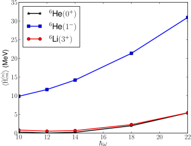
Figure 1: (Color online) Expectation value of the center-of-mass Hamiltonian (71) at the frequency $\hbar\tilde{\omega}=\hbar\omega$. Three different states are shown – the $J^{\pi}=0^{+}$ ground state of ⁶He, the $J^{\pi}=1^{-}$ excited state of ⁶He and the $J^{\pi}=3^{+}$ excited state of ⁶Li. All states are assumed to be the lowest eigenstates of the center-of-mass Hamiltonian in Eq. (71) with $n=0$.

Figure 1 shows the expectation value of the center-of-mass Hamiltonian (71) at the frequency $\hbar\tilde{\omega}=\hbar\omega$ for the three states in question. It is assumed that all states are degenerate with the ground state with $n=0$. The $J^{\pi}=0^{+}$ state of ⁶He and the $J^{\pi}=3^{+}$ state of ⁶Li shows the expected behavior as observed in Hagen et al. (2009a, 2010a). The expectation value vanishes for $\hbar\omega\approx 12$ MeV, but not in general. The expectation value with respect to the $J^{\pi}=1^{-}$ state however, does not vanish for any frequency. It is clearly wrong to assume that it is the ground state of the center-of-mass Hamiltonian (71).

Instead, let us assume that it is the first excited state of the center-of-mass Hamiltonian (71) with $n=1$ . This would make it a $p$ state with negative parity which gives a $J^{\pi}=1^{-}$ state when coupled to a $J^{\pi}=0^{+}$ intrinsic state. If this is the case, it will be a spurious center-of-mass excitation where the intrinsic wave function is degenerate with the intrinsic ground state.

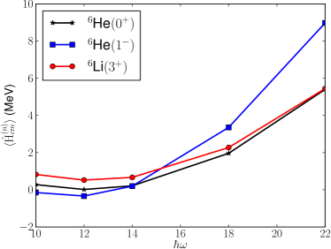
Figure 2: (Color online) Expectation value of the center-of-mass Hamiltonian (71) at the frequency $\hbar\tilde{\omega}=\hbar\omega$. Three different states are shown – the $J^{\pi}=0^{+}$ ground state of ⁶He, the $J^{\pi}=1^{-}$ excited state in ⁶He and the $J^{\pi}=3^{+}$ excited state in ⁶Li. The positive parity states are assumed to be the lowest eigenstates of the center-of-mass Hamiltonian (71) with $n=0$, while the negative parity state is assumed to be the first excited state of the center-of-mass Hamiltonian (71) with $n=1$.

Figure 2 shows the same information as Fig. 1, only now the $J^{\pi}=1^{-}$ state in ⁶He is assumed to be the first excited state of the center-of-mass Hamiltonian (71) with $n=1$. The expectation value now vanishes for all three states at $\hbar\omega\approx 12$ MeV.

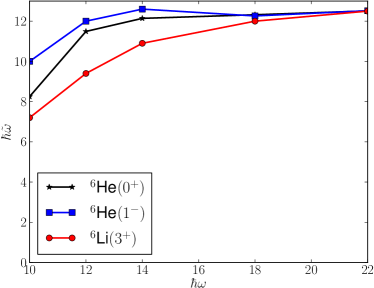
Figure 3: (Color online) Center-of-mass frequency as calculated by the description in Hagen et al. (2009a, 2010a) as a function of the oscillator parameter $\hbar\omega$. Three different states are shown – the $J^{\pi}=0+$ ground state of ⁶He, the $J^{\pi}=1^{-}$ excited state in ⁶He and the $J^{\pi}=3^{+}$ excited state in ⁶Li. The positive parity states are assumed to be the lowest eigenstates of the center-of-mass Hamiltonian (71) with $n=0$, while the negative parity state is assumed to be the first excited state of the center-of-mass Hamiltonian with $n=1$.

Under these assumptions, the appropriate $\hbar\tilde{\omega}$ is calculated using Eq. (72). As seen in Fig. 3, where $\hbar\tilde{\omega}$ is plotted as a function of $\hbar\omega$, the frequency of the center-of-mass Hamiltonian is approximately independent of the frequency of the underlying harmonic oscillator basis for all three states.

Finally, the expectation values are calculated using Eq. (71). The results are shown in Fig. 4.

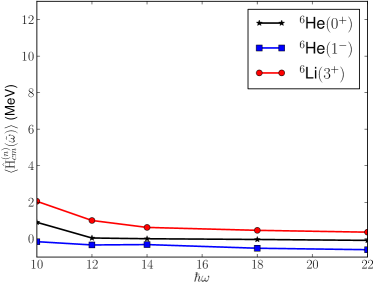
Figure 4: (Color online) The expectation value of the center-of-mass Hamiltonian (71) is calculated at the center-of-mass frequency $\hbar\tilde{\omega}$ for the $J^{\pi}=0+$ ground state of ⁶He, the $J^{\pi}=1^{-}$ excited state in ⁶He and the $J^{\pi}=3^{+}$ excited state in ⁶Li. The positive parity states are assumed to be the lowest eigenstates of the center-of-mass Hamiltonian (71) with $n=0$, while the negative parity state is assumed to be the first excited state of the center-of-mass Hamiltonian with $n=1$.

From these results, we can draw a couple of conclusions. First, since the expectation values are approximately zero, this shows that our assumptions were valid. All states are approximate eigenstates of the center-of-mass Hamiltonian (71). This means that the total wave function separates into an intrinsic part and a center-of-mass part for all three states. Second, the wave functions for the ground state of ⁶He and the first excited $J^{\pi}=3^{+}$ state of ⁶Li, factorizes into intrinsic states and the ground state of the center-of-mass Hamiltonian. Last, the $J^{\pi}=1^{-}$ state in ⁶He factorizes into the intrinsic ground state and the first excited state of the center-of-mass Hamiltonian. It is identified as a spurious center-of-mass excitation and should be removed from the spectrum.

Ideally, one should go through the entire procedure outlined above to make sure that the calculated state is not a spurious center-of-mass excitation. In practice, it is only necessary to verify that the center-of-mass energy $E^{(0)}_{cm}(\hbar\omega)$ vanishes for some value of $\hbar\omega$.

There are several reasons why the results in this section are only approximate. First, the method used to calculate expectation values is not exact. Second, the single-particle space employed in the calculations is cut off at some maximum energy. Although it is verified that the total energy is converged with respect to this cutoff, properties of the wave function might require higher cutoffs. Third, the results obtained by the coupled-cluster machinery are truncated both in the coupled-cluster expansion and in the operator used to define the diagonalization space. Finally, the interaction used in these calculations has been evolved using SRG transformations. The three- and many-body forces induced by this transformation have not been included in these calculations. If one assumes that the first two items yield small deviations from zero, then it might be possible to use this to evaluate how good the coupled-cluster truncations are and say something about the current level of approximation. However, one will need to incorporate $4$p-$2$h corrections to analyze this further.

The purpose of this section has been to show that it is possible to identify and exclude spurious center-of-mass excitations for both ground and excited states calculated with EOM-CC theory. The wave function factorizes, to a very good approximation, into an intrinsic part and a harmonic oscillator eigenfunction for the center-of-mass coordinate. To deternine why this is the case will require additional research and is beyond the scope of this article.

IV.3 Applications to ⁶Li and ⁶He

For any given reference nucleus, there are only three nuclei accessible to the 2PA-EOM-CC method. Using ⁴He as the reference, one can add two protons to calculate properties of ⁶Be, two neutrons for ⁶He and finally a proton and a neutron to calculate properties of ⁶Li. Of these, only ⁶Li and ⁶He are stable with respect to nucleon emission and will be the focus of this section. The structures of ⁶Li and ⁶He differ markedly. This is important, because the quality of the current level of approximation will inevitably depend on the structure of the nucleus under investigation.

⁶Li is well bound and has four bound states below the nucleon emission threshold at $4.433$ MeV Tilley et al. (2002). The ground state has spin parity assignment $J^{\pi}=1^{+}$, while the first excited states have $J^{\pi}=3^{+}$, $2^{+}$ and $0^{+}$. The $J^{\pi}=0^{+}$ ground state in ⁶He has a two neutron halo structure, bound by only $800$ keV Tilley et al. (2002) compared to ⁴He. There are no bound excited states, only a narrow resonance at $1.710$ MeV Tilley et al. (2002), and recently also resonances at $2.6$ and $5.3$ MeV Mougeot et al. (2012)have been documented.

First, let us look at convergence with respect to the size of the model space. Coupled-cluster theory is based on a finite basis expansion, where $N_{\textrm{max}}$ effectively determines the numerical cutoff. The cutoff is increased until the corrections are so small that the uncertainties in the method dominate the error budget. Typically the corrections are down to a tenth of a percentage of the total binding energy. Extrapolations to infinite model spaces Furnstahl et al. (2012); More et al. (2013) have not been performed here but will be included in future work.

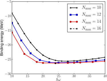
Figure 5: (Color online) Ground state energy of ⁶Li as a function of the oscillator parameter $\hbar\omega$ and the size of the model space $N_{\textrm{max}}$ (see text for details).

Figure 5 shows the calculated total binding energy of ⁶Li as a function of the oscillator frequency $\hbar\omega$. Different lines correspond to different model spaces. At $N_{\textrm{max}}=16$, there is a shallow minimum around $\hbar\omega=24$ MeV and, in a $10$-MeV range including this minimum, the binding energy varies by approximately $100$ keV. This is less than half a percentage of the total energy. At low frequencies, the energy deviates substantially from the minimum, due to the lack of resolution in the single-particle space.

Note that the gain in binding energy when going from $N_{\textrm{max}}=14$ to $N_{\textrm{max}}=16$ is also very small, about $40$ keV. The binding energy of ⁶Li is converged with respect to the size of the model space ($N_{\textrm{max}}$) and the energy at $\hbar\omega=24$ MeV will be tabulated.

The picture is largely identical for the binding energy of ⁶He, only the minimum in energy occurs at $\hbar\omega=20$ MeV. Here the difference in energy between the two largest model space is about $140$ keV.

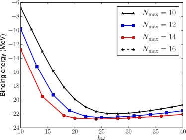
Figure 6: (Color online) The total energy of the first excited $J^{\pi}=3^{+}$ state of ⁶Li as a function of the oscillator parameter $\hbar\omega$ and the size of the model space $N_{\textrm{max}}$ (see text for details).

Figure 6 shows that the excited states follow the same pattern of convergence as the ground states. Here the total energy of the $J^{\pi}=3^{+}$ state in ⁶Li is plotted as a typical example. As before, the energy is plotted as a function of $\hbar\omega$ and different lines correspond to different values of $N_{\textrm{max}}$. In this section, the excitation energy will be defined as

$$E_{\rm x}(\hbar\omega)=E_{J^{\pi}}(\hbar\omega)-E_{\rm gs}(\hbar\omega),$$ (73)

where $E_{J^{\pi}}(\hbar\omega)$ is the total energy of the excited state with spin-parity assignment $J^{\pi}$, calculated at the oscillator frequency $\hbar\omega$. Moreover, $E_{\rm gs}(\hbar\omega)$ is the ground-state energy calculated at the same frequency.

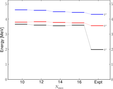
Figure 7: (Color online) Excitation energy for selected states of ⁶Li, as a function of the size of the model space defined by $N_{\textrm{max}}$. The rightmost column shows the experimental values from Tilley et al. (2002).

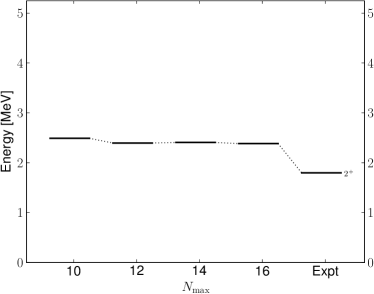
Figure 8: Excitation energy for the first excited $J^{\pi}=2^{+}$ state of of ⁶He, as a function of the size of the model space defined by $N_{\textrm{max}}$. The rightmost column shows the experimental value from Tilley et al. (2002).

In Fig. 7, the convergence pattern of the excitation energies for selected states in the spectrum of ⁶Li is shown. The horizontal axis denotes the size of the model space, where the values in the rightmost column are the experimental values Tilley et al. (2002). All excitation energies have been calculated at $\hbar\omega=24$ MeV, which correspond to the minimum of the ground-state energy. There is very little model space dependence at $N_{\textrm{max}}=16$ and none of the states shown are classified as spurious center-of-mass excitations according to the prescription in Sec. IV.2. A second $J^{\pi}=1^{+}$ state was found higher in the spectrum, but this state was found to be a spurious state and was therefore excluded.

In Fig. 8, an equivalent plot for the first $J^{\pi}=2^{+}$ excited state in ⁶He is shown. This result is also converged with respect to the size of the model space. No significant center-of-mass contamination was found in either this state or the ground state. As already discussed a low-lying $J^{\pi}=1^{-}$ state was also found, but was identified as a spurious center-of-mass excitation. Note that all excitation energies for ⁶He were calculated at $\hbar\omega=20$ MeV.

Let us also look at some properties of the wave function. Although it is not an observable, other expectation values might be more sensitive to changes in the wave function than the energy.

First, the partial norms are defined by

$$n(2p0h) =\frac{1}{2}\sum_{ab}(2J+1)\left(r^{ab}(J)\right)^{2}$$ (74)

$$n(3p1h) =\frac{1}{6}\sum_{\begin{subarray}{c}abci\\ J_{ab}J_{abc}\end{subarray}}\left(2J_{abc}+1\right)\left(r_{i}^{abc}(J_{ab},J_{abc},J)\right)^{2},$$ (75)

where $n(2p0h)+n(3p1h)=1$. The amplitudes $r^{ab}(J)$ and $r_{i}^{abc}(J_{ab},J_{abc},J)$ are the spherical amplitudes defined in Eqs. (103) and (105), respectively, while $J_{x}$ are angular momentum labels. Note that the angular momentum factors are included so the partial norms are consistent between the coupled and uncoupled schemes. These norms quantify the part of the wave function in $2$p-$0$h and $3$p-$1$h configurations, respectively. Note also that they differ in how they are defined from those used in Hagen et al. (2012b), where the $\frac{1}{2}$ and $\frac{1}{6}$ prefactors were not used. This gave a larger $3$p-$1$h norm than those in this work, due to a significant overcounting of the $3$p-$1$h amplitudes.

Second, the total weights are defined by

$$w^{ab}_{pw} =\frac{2J+1}{2}\sum_{a,b}\left[\left(r_{pw}^{ab}(J)\right)^{2}+\left(r_{pw}^{ba}(J)\right)^{2}\right],$$ (76)

where the label $pw$ identifies the partial wave content of the weight. The sum is over all configurations with this partial wave content, because the weights of individual configurations are not stable. In addition, spin-orbit partners are not distinguished.

State	$n(2p0h)$	Dominant configuration(s)	Weight(s)
6Li($1^{+}$)	$0.91$	$(p)^{2}$, $(d)^{2}$	$0.83$, $0.02$
6Li($3^{+}$)	$0.90$	$(p)^{2}$,$(pf)$	$0.81$, $0.04$
6Li($0^{+}$)	$0.88$	$(p)^{2}$	$0.87$
6Li($2^{+}$)	$0.91$	$(p)^{2}$, $(pf)$, $(d)^{2}$	$0.77$, $0.07$, $0.02$
6He($0^{+}$)	$0.88$	$(p)^{2}$	$0.87$
6He($2^{+}$)	$0.90$	$(p)^{2}$, $(pf)$	$0.87$, $0.02$
6He($1^{-}$)	$0.84$	$(ps)$, $(pd)$	$0.49$, $0.34$

Table 4: This table shows the $2$p-$0$h partial norms (74), as well as the dominant configurations for calculated states in both ⁶Li and ⁶He. The weights are calculated according to Eq. (76) where all nodes for a given partial wave contribute to the sum and spin-orbit partners are not distinguished.

In Table 4 partial norms and dominant weights of selected states in ⁶Li and ⁶He are listed. A few comments are in order. First, all physical states are consistent with the shell-model picture, where the dominant contributions to the wave function come from two valence nucleons in the $p$ shell. Only the $J^{\pi}=1^{-}$ state in ⁶He contains contributions from the $sd$ shell, but this is natural as no pure $p$ shell configuration will give a negative-parity state. It is also a spurious center-of-mass excitation and is excluded from the spectrum. Second, the $2$p-$0$h norm for all physical states are around $0.9$. Only the spurious state has a significantly lower norm at $0.84$. The remaining $0.1$ in the $3$p-$1$h norms are needed to relax the reference wave function as it changes due to the presence of the extra nucleons. Finally, the wave function of the ground state of ⁶He and the first excited $J^{\pi}=0^{+}$ state in ⁶Li are very similar. This is not surprising, since they can be viewed as two parts of a degenerate isospin triplet.

6Li	Expt.	N3LO	NCSMNavrátil and Caurier (2004)
		($\Lambda=500\mathrm{MeV}$)
$\mathrm{E_{gs}}(1^{+})$	$-31.993$	$-28.44(5)$	$-28.5(5)$
$\mathrm{E_{gs}}(1^{+})$	$0.0$	$0.0$	$0.0$
$\mathrm{E_{x}}(3_{1}^{+})$	$+2.186$	$+3.60(4)$	$+2.91(3)$
$\mathrm{E_{x}}(0_{1}^{+})$	$+3.562$	$+3.76(3)$	$+3.30(10)$
$\mathrm{E_{x}}(2_{1}^{+})$	$+4.312$	$+4.44(4)$	$+4.10(15)$
6He
$\mathrm{E_{gs}}(0^{+})$	$-29.270$	$-25.51(14)$	$-26.2(5)$
$\mathrm{E_{gs}}(0^{+})$	$0.0$	$0.0$	$0.0$
$\mathrm{E_{x}}(2^{+})$	$1.797$	$2.35(4)$

Table 5: Binding energies and excitation energies for selected states of ⁶Li and ⁶He with estimated numerical uncertainties. The uncertainties in our results are the differences between the values for the two largest model spaces. The data is compared to NCSM results Navrátil and Caurier (2004) in the rightmost column, where the parenthesis list extrapolation errors and experimental data in the leftmost column. All experimental data are from Tilley et al. (2002).

Table 5 shows results with estimated numerical uncertainties for the ground and selected excited states of both ⁶He and ⁶Li. For comparison, both experimental values and results from a no-core shell-model (NCSM) calculation Navrátil and Caurier (2004) are tabulated where data are available. Note that the results from the NCSM calculation are based on the same interaction as the results from this work, but the interaction is renormalized using the procedure defined in Suzuki and Lee (1980) before the diagonalization was performed. In addition, the final results were extrapolated to an infinite model space.

Let us discuss the uncertainties indicated by the parenthesis in the table. For the results from this work, listed in the second column, the numbers in parenthesis give the difference in energy between the two largest model spaces. The results from Navrátil and Caurier (2004) give the extrapolation errors in the last column, while the experimental energies Tilley et al. (2002) in the first column are listed without uncertainties.

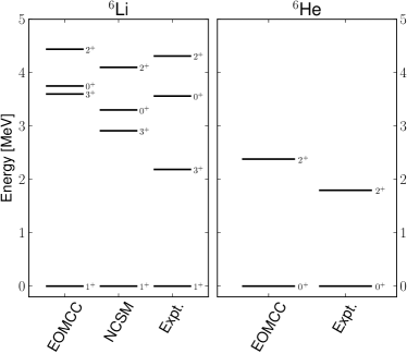
Figure 9: Excitation levels of selected states in ⁶Li and ⁶He, calculated using 2PA-EOM-CC(this work) and NCSM Navrátil and Caurier (2004), compared to experimental Tilley et al. (2002) values.

Figure 9 shows a graphical representation of the data in Table 5. Compared to the results from the NCSM calculation, our results are quite promising. First, the ground-state energy of ⁶Li is well within the uncertainties of the “exact” result, while the ground-state energy of ⁶He is just outside. The difference between the two nuclei can be explained by the extended spatial distribution of ⁶He. Additional correlations are necessary to account for this structure. Although the $\alpha$ core in ⁶He is expected to stay largely unchanged when adding two neutrons, the distribution of these extra neutrons are biased in one direction. This results in a skewed center of mass compared to the center of mass of the $\alpha$ core alone. Additional correlations are necessary to absorb the resulting oscillations of the $\alpha$ core with respect to the combined center of mass. The spatial distribution of ⁶Li is tighter, so this effect is not that prominent. Second, the ordering of excited states in ⁶Li is reproduced. Finally, the excitation energies are consistently overestimated. For the first $J^{\pi}=0^{+}$ and $2^{+}$ states the differences between the two calculations are small enough to be ascribed to differences in the interaction used. But the difference for the $J^{\pi}=3^{+}$ state, however, is too large for such a simple explanation. Neither the partial norms nor the total weights listed in Table 4 provide any hint of explanation for this discrepancy. About $90$ % of the wave function is in $2$p-$0$h configurations, which is comparable to the ground state. The wave function is dominated by configurations where both nucleons are in $p$ orbitals, which is consistent with the shell-model picture. Furthermore, the level of convergence for this state is no different from the other excited states. As noted in Sec. IV.2, with the SRG evolved interaction, the $J^{\pi}=3^{+}$ state had a slight center-of-mass contribution, which was not present in the other states. This was illustrated in Fig. 4, but a similar calculation using the bare interaction was too computationally intensive to extract any meaningful information. I include it because it might indicate that additional correlations are needed in the calculation, either in the reference or the EOM operator. This matter needs to be investigated further, but currently the implementation will not allow model spaces large enough for a converged description of the center-of-mass admixture in the final wave function.

Using the in-medium similarity renormalization group (IM-SRG), Tsukiyama et al. (2012) performed a similar study with a softer interaction. Here, the $J^{\pi}=3^{+}$ state in ⁶Li is reproduced on the same level of accuracy as for the other bound states.

Let us also look at some of the differences between the results in this work and the experimental data. First, all excitation energies are overestimated compared to data. Again, the $J^{\pi}=3^{+}$ states is exceptional, but this has been discussed in detail by Navrátil and Caurier (2004). The matter was resolved by the inclusion of three-nucleon forces Navrátil et al. (2007), which also brought the binding energy very close to data.

There is also an $\approx 500$-keV difference for the $J^{\pi}=2^{+}$ resonance in ⁶He, but here the effects of three-body forces might be less important. This state was also investigated using a chiral interaction with a different cutoff of $600$ MeV. With this interaction, the excitation energy of this state was unchanged. That was not the case for the excited states in ⁶Li, where especially the $J^{\pi}=3^{+}$ state turned out to be very cutoff dependent. Since the $J^{\pi}=2^{+}$ state in ⁶He is a resonance, the continuum is expected to have a larger impact. The current single-particle basis cannot handle the description of both bound, resonance and continuum states that are necessary in this case. These effects have not been included in this calculation, as the focus has been on properties of the method rather than the interaction. The method has been extended to include a Gamow basis as in Michel et al. (2004) and Hagen et al. (2007b). It has already been applied to ²⁶F Lepailleur et al. (2013), but a comprehensive discussion is beyond the scope of this article.

Summing up this section, I would like to point out that for well-bound states, with simple structure, the current approximation will yield total energies comparable to exact diagonalization. The calculations can be done in sufficiently large model spaces for the results to be converged for six nucleons, but for certain states, the effects of $4$p-$2$h configurations need to be investigated. To compare to experimental data, however, both three-nucleon forces and continuum degrees of freedom are necessary.

IV.4 Applications to ¹⁸O and ¹⁸F

When ¹⁶O is used as a reference state, the three isobars ¹⁸O, ¹⁸F, and ¹⁸Ne are reachable by the 2PA-EOM-CCSD method. All have well-bound ground states and a rich spectra of bound excited states below their respective nucleon emission thresholds. The spectrum of ¹⁸F is especially rich, as the exclusion principle does not affect the placement of nucleons in the $sd$ shell. The proton-neutron interaction is responsible for the compressed spectrum in the fluorine isotope, while strong pairing effects in ¹⁸O result in a lower ground-state energy. In both ¹⁸O and ¹⁸Ne the spectra are opened up and the first excited states are higher in energy. Our current focus is on convergence and the viability of this method. Thus, ¹⁸Ne is not explicitly discussed, as results are similar to those of ¹⁸O.

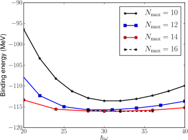
Figure 10: (Color online) The ground-state energy of ¹⁸O as a function of the oscillator parameter, $\hbar\omega$. Different lines correspond to different model spaces, parametrized by the variable $N_{\textrm{max}}$ (69).

Let us first look at the convergence of the binding energy of ¹⁸O. Figure 10 shows the ground-state energy of ¹⁸O as a function of the oscillator parameter $\hbar\omega$. The different lines correspond to different model spaces, parametrized by the variable $N_{\textrm{max}}$ (69). A shallow minimum develops around $\hbar\omega=32$ MeV, where the energy is converged with respect to the size of the model space. The difference in energy is about $20$ keV when the size of the model space is increased from $N_{\textrm{max}}=14$ to $N_{\textrm{max}}=16$. For a wide range of values around the minimum, the ground state energy shows very little dependence on the $\hbar\omega$ parameter. Thus, the result is converged with respect to the size of the model space.

A similar result is obtained for the ground-state energy of ¹⁸F, where the difference in energy is around $160$ keV between the two largest model spaces. This is almost an order of magnitude larger than for the ground state of ¹⁸O but is still well within $1\%$ of the total energy.

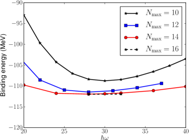
Figure 11: (Color online) The total energy of the $J^{\pi}=3+$ state in ¹⁸O as a function of the oscillator parameter, $\hbar\omega$. Different lines correspond to different model spaces, parametrized by the variable $N_{\textrm{max}}$ (69).

Figure 11 shows the total energy of the first excited $J^{\pi}=3^{+}$ state in ¹⁸O for different model spaces. Here, a shallow minimum develops at $\hbar\omega=28$ MeV. Moreover, this state is very well converged, with a difference in energy of only about $25$ keV between calculations in the two largest model spaces. It is clear that the rate of convergence differs for different values of $\hbar\omega$. When excitation energies are wanted, different choices of $\hbar\omega$ lead to different results. Let us discuss two options to evaluate the excitation energy. First, the total energies can be treated as variational results, where the lowest energy for the ground state and the lowest energy for the $J^{\pi}=3^{+}$ excited state, are chosen. Thus, at $N_{\textrm{max}}=16$ the excitation energy can be calculated as

$$E_{x}(3^{+})=E_{3^{+}}(28\mathrm{MeV})-E_{0_{1}^{+}}(32\mathrm{MeV}),$$ (77)

where $E_{3^{+}}(28\mathrm{MeV})$ is the total energy of the $J^{\pi}=3^{+}$ excited state, calculated at $\hbar\omega=28$ MeV, while $E_{0_{1}^{+}}(32\mathrm{MeV})$ is the ground-state energy calculated at $\hbar\omega=32$ MeV.

Second, the same value of $\hbar\omega$ can be used for both energies, typically where the ground state has a minimum. Thus, for the current case the excitation energy is calculated as

$$E_{x}(3^{+})=E_{3^{+}}(32\mathrm{MeV})-E_{0_{1}^{+}}(32\mathrm{MeV}).$$ (78)

The difference in energy between these two options is minimal if sufficiently large model spaces are used, but it will have a significant impact on the rate of convergence.

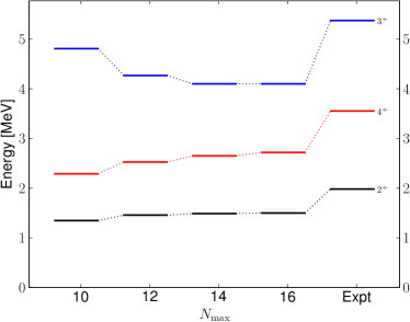
Figure 12: (Color online) The excitation energies of the first $J^{\pi}=2^{+}$, $3^{+}$, and $4^{+}$ excited states in ¹⁸O where the best values for $\hbar\omega$ has been chosen for each state. The different columns represent different model spaces parametrized by the variable $N_{\textrm{max}}$ (69). The rightmost column contains experimental values from Tilley et al. (1995).

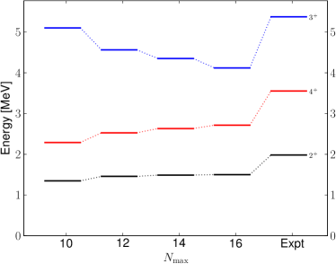
Figure 13: (Color online) The excitation energies of the first $J^{\pi}=2^{+}$, $3^{+}$, and $4^{+}$ excited states in ¹⁸O for $\hbar\omega=32$ MeV. The different columns represent different model spaces parametrized by the variable $N_{\textrm{max}}$ (69). The rightmost column contains experimental values from Tilley et al. (1995).

The effect is best viewed in Figs. 12 and 13, where the excitation energies of the first $J^{\pi}=2^{+}$, $3^{+}$, and $4^{+}$ excited states in ¹⁸O as functions of the size of the model space, are plotted. In Fig. 12, the excitation energies are calculated according to Eq. (77), while they are calculated according to Eq. (78) in Fig. 13. For ¹⁸O, this choice will affect only the $J^{\pi}=3^{+}$ state, as the other states all have minimum values at $\hbar\omega=32$ MeV. The effect is significant, but the first approach of Fig. 12 correctly depicts the level of convergence of the excited states and will be used in the following.

As in the previous section, let us look at some properties of the wave functions.

State	$n(2p0h)$	Dominant configuration(s)	Weight(s)
18O($0^{+}_{1}$)	0.87	$(d)^{2}$, $(s)^{2}$	0.75,0.12
18O($0^{+}_{2}$)	0.87	$(s)^{2}$, $(d)^{2}$	0.80, 0.07
18O($0^{+}_{3}$)	0.87	$(d)^{2}$, $(f)^{2}$	0.85, 0.02
18O($2^{+}_{1}$)	0.88	$(d)^{2}$, $(sd)$	0.55, 0.32
18O($2^{+}_{2}$)	0.88	$(sd)$, $(d)^{2}$	0.61, 0.27
18O($2^{+}_{3}$)	0.88	$(d)^{2}$, $(sd)$	0.76, 0.11
18O($3^{+}_{1}$)	0.88	$(sd)$	0.88
18O($4^{+}_{1}$)	0.88	$(d)^{2}$	0.88
18O($1^{-}_{1}$)	0.83	$(dp)$,$(sp)$, $(df)$	0.34, 0.26, 0.23
18O($2^{-}_{1}$)	0.84	$(dp)$,$(df)$,$(sp)$	0.50, 0.32, 0.02
18O($3^{-}_{1}$)	0.82	$(dp)$,$(df)$,$(sf)$	0.42, 0.20, 0.19
18F($0^{+}_{1}$)	0.87	$(d)^{2}$, $(s)^{2}$	0.70, 0.16
18F($1^{+}_{1}$)	0.89	$(d)^{2}$, $(s)^{2}$,$(f)^{2}$,$(sd)$	0.61, 0.20, 0.02, 0.01
18F($2^{+}_{1}$)	0.88	$(sd)$, $(d)^{2}$,$(dg)$,$(f)^{2}$	0.59, 0.24, 0.02, 0.01
18F($3^{+}_{1}$)	0.88	$(sd)$, $(d)^{2}$,$(dg)$	0.58, 0.26, 0.02
18F($4^{+}_{1}$)	0.88	$(d)^{2}$	0.88
18F($5^{+}_{1}$)	0.88	$(d)^{2}$, $(sg)$, $(dg)$	0.86, 0.01, 0.01

Table 6: This table shows the $2$p-$0$h partial norms(74), as well as the dominant configurations for calculated states in both ¹⁸O and ¹⁸F. The weights are calculated according to Eq. (76) where all nodes for a given partial wave contribute to the sum and spin-orbit partners are not distinguished.

First, the partial norms defined in Eq. (74) and the total weights (76) of the different configurations are calculated. The results are tabulated in Table 6. All positive-parity states have two nucleons in the $sd$ shell and are consistent with the standard shell model picture. As in the previous section, all $2$p-$0$h norms are close to $0.90$, except for the negative-parity states which are closer to $0.80$. The negative-parity states are dominated by cross-shell configurations as these are the only $2$p-$0$h configurations that can give a negative parity. $3$p-$1$h excitations from the $p$ shell give a substantial contribution to the $3$p-$1$h norm.

Second, the center-of-mass contamination of each wave function was analyzed according to the prescription in Sec. IV.2. Of the states tabulated in Table 6, four states had a significant center-of-mass contamination. Let us, first, focus on the three negative-parity states in ¹⁸O.

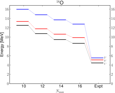
Figure 14: (cClor online) The excitation energies of the first $J^{\pi}=1^{-}$, $2^{-}$, and $3^{-}$ excited states in ¹⁸O for $\hbar\omega=32$ MeV. The different columns represent different model spaces parametrized by the variable $N_{\textrm{max}}$ (69). The rightmost column contains experimental values from Tilley et al. (1995).

Figure 14 shows the excitation energies of the negative-parity states in ¹⁸O and they are not yet converged at $N_{\textrm{max}}=16$. Although they had a large center-of-mass component, it was not possible to establish what kind of center-of-mass excitations these states corresponded to. Calculations in larger model spaces needs to be performed to correctly describe these states. However, it is also necessary to include $4$p-$2$h correlations to get these states right. This can be understood by examining how negative-parity states can occur in ¹⁸O. First, they can be produced by placing one neutron in the $sd$ shell, while the other is placed in the $pf$ shell. If this was the dominant configuration, the current truncation would have been enough. Second, they can also be produced by placing two neutrons in the $sd$ shell and excite a nucleon from the $p$ shell up to the $sd$ shell. If these kind of excited configurations are comparable in energy to the first kind, $3$p-$1$h configurations start to dominate and $4$p-$2$h configurations are necessary for the proper relaxation of the wave function. One can ask whether the center-of-mass contamination would change if these configurations were included and whether it is a result of a poorly converged wave function, but this will be a topic for future work.

In the spectrum of ¹⁸O, there are three bound $J^{\pi}=0^{+}$ and $2^{+}$ states. The second $J^{\pi}=0^{+}$ state is especially interesting for this method, as it is a $4$p-$2$h state Ellis and Engeland (1970). In the shell-model language, it is an intruder state, because configurations outside the $sd$ shell are important to get this state right. As the current implementation includes only the $3$p-$1$h configurations, this state can provide clues as to what type of behavior can be expected from states that are not converged with respect to the level of approximation.

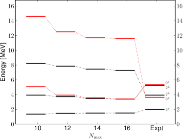
Figure 15: (Color online) The excitation energies of the first few $J^{\pi}=0+$ and $2+$ states in ¹⁸O for $\hbar\omega=32$ MeV. The different columns represents different model spaces parametrized by the variable $N_{\textrm{max}}$ (69). The rightmost column contains experimental values from Tilley et al. (1995).

Table 6 lists three $J^{\pi}=0^{+}$ states in ¹⁸O and none of them stands out. They all have similar partial norms of around $88$ % and are dominated by two neutrons in $d_{5/2}$, $s_{1/2}$, and $d_{3/2}$, respectively. In Fig. 15 the convergence patterns for these states are plotted, along with those of the three $J^{\pi}=2^{+}$ states. All states show similar level of convergence and it is not possible to single out one of the states. However, if we look at the center-of-mass contamination of these states, the third $J^{\pi}=0^{+}$ shows a large contamination, while the other states show almost none. Assuming that missing many-body correlations will manifest as larger center-of-mass contaminations in the final wave functions, this state is associated with the experimental second $J^{\pi}=0^{+}$ state. The calculated second $J^{\pi}=0^{+}$ is closer in energy, but including effects of three-nucleon forces pushes this state higher in energy and very close to the experimentally observed $J^{\pi}=0^{+}$ state at $5.34$ MeV. Hagen et al. (2012a). A similar effect occurs among the $J^{\pi}=2^{+}$ excited states, but it is less prominent. Here, the center-of-mass contamination were negligible for all but the third $J^{\pi}=2^{+}$ state, but even here, the contamination was small compared to the third $J^{\pi}=0^{+}$ state.

Let us summarize the discussion of missing many-body correlations. Three different markers have been identified to indicate missing physics. Unfortunately, none of them can be used quantitatively and all must be evaluated simultaneously to form a general picture. First, the partial norms can be used to differentiate among different states. From these calculations it seems that a $2$p-$0$h norm of around $90$ % is the standard. A lower partial norm, might indicate the need for $4$p-$2$h or higher correlations.

Second, we look at the convergence patterns and if energies converge slowly, this probably means that something is missing from the calculation. In weakly bound states, for example, continuum effects result in the need for additional resolution in the single-particle basis. Finally, we look at the level of center-of-mass contamination present in the wave function. Either the state can be identified as a spurious center-of-mass excitation or a small non-zero center-of-mass component might indicate missing correlations. None of these arguments can be analyzed in detail before $4$p-$2$h configurations are included. This is a work in progress, but, computationally, it will only be possible to include these configurations in a small single-particle space. If the $3$p-$1$h and $4$p-$2$h configurations are defined only in a so-called active space around the Fermi level, the computational cost might be manageable. This has been done successfully in Gour et al. (2005) and should prove to be a valuable approximation also in this method. The formation of a correlated $\alpha$ cluster around the Fermi level is important in this mass region and can hopefully be accounted for using a minimal set of $4$p-$2$h configurations.

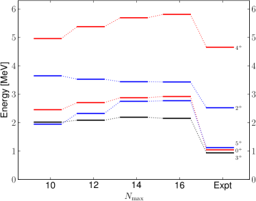
Figure 16: (Color online) The excitation energies of the first $J^{\pi}=0^{+}$, $2^{+}$, $3^{+}$, $4^{+}$, and $5^{+}$ states in ¹⁸F, calculated at $\hbar\omega=30$ MeV. The different columns represents different model spaces parametrized by the variable $N_{\textrm{max}}$ (69). The rightmost column contains experimental values from Tilley et al. (1995).

Let us also look at the convergence of selected states in ¹⁸F. Figure 16 shows the excitation energy of the first few states in ¹⁸F for different model spaces. Here all states are relatively well converged, with only the $J^{\pi}=4^{+}$ state showing some model space dependence at $N_{\textrm{max}}=16$. None of these states have significant center-of-mass contamination and all partial norms are on the same level as can be seen in Table 6. This table also shows there is a slight contribution to the wave function from outside the $sd$ shell.

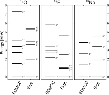
Figure 17: Excitation energies for selected states in ¹⁸O, ¹⁸F, and ¹⁸Ne compared to experimental values from Tilley et al. (1995).

Figure 17 shows the excitation spectra of ¹⁸O, ¹⁸F, and ¹⁸Ne. Only states that are considered good are plotted and compared to data.

18O	Expt.	N3LO
		($\Lambda=500\mathrm{MeV}$)
$\mathrm{E_{gs}}(0^{+})$	$-139.807$	$-130.00(2)$
$\mathrm{E_{gs}}(0^{+}_{1})$	$0.0$	$0.0$
$\mathrm{E_{x}}(2^{+}_{1})$	$+1.982$	$+1.50(1)$
$\mathrm{E_{x}}(4^{+}_{1})$	$+3.554$	$+2.72(7)$
$\mathrm{E_{x}}(0^{+}_{2})$	$+3.633$	NA
$\mathrm{E_{x}}(2^{+}_{2})$	$+3.92$	$+3.38(2)$
$\mathrm{E_{x}}(2^{+}_{3})$	$+5.255$	$+7.27(18)$
$\mathrm{E_{x}}(0^{+}_{3})$	$+5.336$	$+3.40(15)$
$\mathrm{E_{x}}(3^{+}_{1})$	$+5.3778$	$+4.12(1)$
18F
$\mathrm{E_{gs}}(1^{+})$	$-137.370$	$-129.75(16)$
$\mathrm{E_{gs}}(1^{+})$	$0.0$	$0.0$
$\mathrm{E_{x}}(3^{+})$	$+0.937$	$+2.15(4)$
$\mathrm{E_{x}}(0^{+})$	$+1.041$	$+2.92(4)$
$\mathrm{E_{x}}(5^{+})$	$+1.121$	$+2.77(2)$
$\mathrm{E_{x}}(2^{+})$	$+2.523$	$+3.43(1)$
$\mathrm{E_{x}}(4^{+})$	$+4.652$	$+5.81(12)$
18Ne
$\mathrm{E_{gs}}(0^{+})$	$-132.143$	$-122.56(15)$
$\mathrm{E_{gs}}(0^{+})$	$0.0$	$0.0$
$\mathrm{E_{x}}(2^{+})$	$+1.887$	$+1.43(3)$
$\mathrm{E_{x}}(4^{+})$	$+3.376$	$+2.59(6)$
$\mathrm{E_{x}}(3^{+})$	$+4.561$	$+3.83(4)$

Table 7: Ground- and excited-state energies for the $A=18$ system, compared to experimental data. The experimental energies are from Tilley et al. (1995). The number in parenthesis indicates the level of convergence and is the difference in energy between calculations in the two largest model spaces.

For future comparison, Table 7 lists the numerical values used in Fig. 17, together with the ground-state energies. The uncertainty is calculated as the difference in energy between calculations in the two largest model spaces. The experimental values are from Tilley et al. (1995).

The total binding energy of ¹⁸O is comparable to what was found in Hergert et al. (2013a), where the in-medium similarity renormalization group (IM-SRG) Tsukiyama et al. (2011) method was used to compute the ground-state energies of even oxygen isotopes. Although they used an SRG evolved interaction based on chiral interaction at fourth order by Entem and Machleidt (2003), induced three-nucleon forces were also included in the final calculation to make the results comparable to those in Table 7.

Compared to data, the level ordering in ¹⁸F is reproduced, but the excitation energies are systematically overestimated. Disregarding the missing states in ¹⁸O, the level ordering is also reproduced, but here the excitation energies are systematically underestimated. This is consistent with shell-model calculations Holt et al. (2005); Dong et al. (2011) of these nuclei using different model-space interactions. For results based on the chiral interactions used in this work, the inclusion of three-nucleon forces Hagen et al. (2012a); Holt et al. (2013) gives results that better match experimental data. Recently, Ekström et al. (2013) showed that the effects of three-nucleon forces depends on the low-energy constants used in the parametrization of the chiral potential. To accurately evaluate the quality of these forces will require not only three-nucleon forces and continuum degrees of freedom but also additional correlations in the many-body wave function Volya and Zelevinsky (2005); Hagen et al. (2009b); Otsuka et al. (2010); Hagen et al. (2012a); Hergert et al. (2013b, a).

V Conclusions and outlook

The spherical version of the 2PA-EOM-CCSD method has been presented. This is appropriate for the calculation of energy eigenstates in nuclei that can be described as two particles attached to a closed (sub-)shell reference. The method has been evaluated in both $A=6$ and $A=18$ nuclei, where the results were converged with respect to the single-particle basis.

It was also shown that the wave function from a 2PA-EOM-CCSD calculation separates into an intrinsic part and a Gaussian for the center-of-mass coordinate, not necessarily the ground state of the harmonic oscillator Hamiltonian. Wave functions with significant center-of-mass contamination were either identified as a spurious center-of-mass excitation or were not converged with respect to the current approximation level.

In comparison with a full diagonalization, both ground-state and excited-state energies were in general very accurate. However, one excited state in ⁶Li deviated significantly from the “exact” result, showing the need to include additional correlations like $4$p-$2$h configurations for the accurate treatment of complex states. For simple states, where a $2$p structure is dominant, the current level of truncation is adequate.

Both three-nucleon forces and a correct treatment of the scattering continuum are needed to refine the results.

Appendix A Reduced matrix elements

The reduced matrix elements of a spherical tensor operator $\mathrm{\hat{T}}_{M}^{J}$ of rank $J$ and projection $M$, are defined according to the Wigner-Eckart theorem,

$$\langle\alpha;J_{\alpha}M_{\alpha}|\mathrm{\hat{T}}^{J}_{M}|\beta;J_{\beta}M_{\beta}\rangle=C^{JJ_{\beta}J_{\alpha}}_{MM_{\beta}M_{\alpha}}\langle\alpha;J_{\alpha}||\mathrm{\hat{T}}^{J}||\beta;J_{\beta}\rangle.$$ (79)

Here $\alpha$ and $\beta$ are general labels representing all quantum numbers except angular momentum and its projection, while $J_{\alpha}(M_{\alpha})$ and $J_{\beta}(M_{\beta})$ are the total angular momentum(projection) of the bra and ket states, respectively. The double bars denote reduced matrix elements and does not depend on any of the angular-momentum projections and $C^{JJ_{\beta}J_{\alpha}}_{MM_{\beta}M_{\alpha}}$ is a Clebsch-Gordon coefficient.

In coupled cluster, the unknown amplitudes are the matrix elements of the cluster operator $\mathrm{\hat{T}}^{0}_{0}$,

$$t_{i}^{a} =\langle a;j_{a}m_{a}|\mathrm{\hat{T}}^{0}_{0}|i;j_{i}m_{i}\rangle$$ (80)

$$t_{ij}^{ab} =\langle ab;j_{a}m_{a}j_{b}m_{b}|\mathrm{\hat{T}}^{0}_{0}|ij;j_{i}m_{i}j_{j}m_{j}\rangle$$ (81)

$$\vdots =\vdots,$$ (82)

where the operator sub- and superscriptsidentify the cluster operator as a scalar under rotation. Also, the labels $abij\ldots$, denote single-particle states and we have singled out the angular momentum(projection) in the labels $j_{a}(m_{a})$, and so on.

Now the reduced matrix elements of the cluster operator are defined according to Eq. (79). For example,

$$\langle ab;j_{a}m_{a}j_{b}m_{b}|\mathrm{\hat{T}}^{0}_{0}|ij;j_{i}m_{i}j_{j}m_{j}\rangle=\\ \sum_{\begin{subarray}{c}J_{ab}M_{ab}\\ J_{ij}M_{ij}\end{subarray}}C_{m_{a}m_{b}M_{ab}}^{j_{a}j_{b}J_{ab}}C_{m_{i}m_{j}M_{ij}}^{j_{i}j_{j}J_{ij}}C_{0M_{ij}M_{ab}}^{0J_{ij}J_{ab}}\\ \times\langle ab;j_{a}j_{b};J_{ab}||\mathrm{\hat{T}}^{0}||ij;j_{i}j_{j};J_{ij}\rangle,$$ (83)

where the sum and the first two Clebsch-Gordon coefficients come from the coupling of $j_{a}$ and $j_{b}$ to $J_{ab}$ and of $j_{i}$ and $j_{j}$ to $J_{ij}$, in that specific order This expression is simplified by the explicit evaluation of the third Clebsch-Gordon coefficient

$$C_{0M_{ij}M_{ab}}^{0J_{ij}J_{ab}}=\delta_{J_{ab},J_{ij}=J}\delta_{M_{ab},M_{ij}=M},$$ (84)

where $\delta_{\alpha,\beta}$ is the Kronecker $\delta$. We get

$$\langle ab;j_{a}m_{a}j_{b}m_{b}|\mathrm{\hat{T}}^{0}_{0}|ij;j_{i}m_{i}j_{j}m_{j}\rangle=\\ \sum_{JM}C_{m_{a}m_{b}M}^{j_{a}j_{b}J}C_{m_{i}m_{j}M}^{j_{i}j_{j}J}\langle ab;j_{a}j_{b};J||\mathrm{\hat{T}}^{0}||ij;j_{i}j_{j};J\rangle.$$ (85)

When this specific coupling order is used (left to right) and no confusion will arise, we will use a shorthand notation for the reduced matrix elements, defined by

$$t_{i}^{a}(J) =\langle a;J||\mathrm{\hat{T}}^{0}||i;J\rangle$$ (86)

$$t_{ij}^{ab}(J) =\langle ab;j_{a}j_{b};J||\mathrm{\hat{T}}^{0}||ij;j_{i}j_{j};J\rangle.$$ (87)

The transformations between the reduced amplitudes and the original amplitudes of the cluster operator are defined as

$$t_{i}^{a}(J) =\delta_{j_{a},j_{i}=J}t_{i}^{a}$$ (88)

$$t_{i}^{a} =\delta_{j_{a},j_{i}=J}t_{i}^{a}(J)$$ (89)

$$t_{ij}^{ab}(J) =\frac{1}{\hat{J}^{2}}\sum_{\begin{subarray}{c}m_{a}m_{b}\\ m_{i}m_{j}M\end{subarray}}C_{m_{a}m_{b}M}^{j_{a}j_{b}J}C_{m_{i}m_{j}M}^{j_{i}j_{j}J}t_{ij}^{ab}$$ (90)

$$t_{ij}^{ab} =\sum_{JM}C_{m_{a}m_{b}M}^{j_{a}j_{b}J}C_{m_{i}m_{j}M}^{j_{i}j_{j}J}t_{ij}^{ab}(J),$$ (91)

where we use the convention $\hat{J}=\sqrt{2J+1}$.

As the similarity-transformed Hamiltonian($\mathrm{\bar{H}}$) is a scalar under rotation as well, the shorthand form of its reduced matrix elements are defined analogously,

$$\mathrm{\bar{H}}_{q}^{p}(J) =\langle p;J||\mathrm{\bar{H}}^{0}||q;J\rangle$$ (92)

$$\mathrm{\bar{H}}_{rs}^{pq}(J) =\langle pq;j_{p}j_{q};J||\mathrm{\bar{H}}^{0}||rs;j_{r}j_{s};J\rangle.$$ (93)

The transformations between the original and reduced matrix elements are given by

$$\mathrm{\bar{H}}_{q}^{p}(J) =\delta_{j_{p},j_{q}=J}\mathrm{\bar{H}}_{q}^{p}$$ (94)

$$\mathrm{\bar{H}}_{q}^{p} =\delta_{j_{p},j_{q}=J}\mathrm{\bar{H}}_{q}^{p}(J)$$ (95)

$$\mathrm{\bar{H}}_{rs}^{pq}(J) =\frac{1}{\hat{J}^{2}}\sum_{\begin{subarray}{c}m_{p}m_{q}\\ m_{r}m_{s}M\end{subarray}}C_{m_{p}m_{q}M}^{s_{p}s_{q}J}C_{m_{r}m_{s}M}^{s_{r}s_{s}J}\mathrm{\bar{H}}_{rs}^{pq}$$ (96)

$$\mathrm{\bar{H}}_{rs}^{pq} =\sum_{JM}C_{m_{p}m_{q}M}^{s_{p}s_{q}J}C_{m_{r}m_{s}M}^{s_{r}s_{s}J}\mathrm{\bar{H}}_{rs}^{pq}(J).$$ (97)

The original matrix elements of the similarity-transformed Hamiltonian are defined in Jansen et al. (2011).

The $r$ amplitudes are the matrix elements of the excitation operator in Eq. (51),

$$r^{ab} =\langle ab;j_{a}m_{a}j_{b}m_{b}|\mathrm{\hat{R}}_{M}^{J}|0\rangle$$ (98)

$$r^{abc}_{i} =\langle abc;j_{a}m_{a}j_{b}m_{b}j_{c}m_{c}|\mathrm{\hat{R}}_{M}^{J}|i;j_{i}m_{i}\rangle,$$ (99)

where the operator is now a general tensor operator of rank $J$ and projection $M$. The bra side contains up to three indices and we have to couple three angular momentum vectors to be able to define the reduced amplitudes. Using $r^{abc}_{i}$ as an example, we couple from left to right and get

$$\langle abc;j_{a}m_{a}j_{b}m_{b}j_{c}m_{c}|\mathrm{\hat{R}}_{M}^{J}|i;j_{i}m_{i}\rangle=\\ \sum_{\begin{subarray}{c}J_{ab}M_{ab}\\ J_{abc}M_{abc}\end{subarray}}C_{m_{a}m_{b}M_{ab}}^{j_{a}j_{b}J_{ab}}C_{M_{ab}m_{c}M_{abc}}^{J_{ab}j_{c}J_{abc}}C_{Mm_{i}M_{abc}}^{Jj_{i}J_{abc}}\\ \langle abc;j_{a}j_{b};J_{ab}j_{c};J_{abc}||\mathrm{\hat{R}}^{J}||i;j_{i}\rangle,$$ (100)

where the last Clebsch-Gordon coefficient is due to the Wigner-Eckart theorem. We let the order of the angular-momentum labels on the bra side specify the coupling order, where $j_{a}$ and $j_{b}$ couples to $J_{ab}$. In turn, $J_{ab}$ and $j_{c}$ couples to $J_{abc}$. When this coupling order has been used and no confusion will arise, we will use the shorthand notation for the reduced elements, defined by

$$r^{ab}(J) =\langle ab;j_{a}j_{b};J||\mathrm{\hat{R}}^{J}||o\rangle$$ (101)

$$r^{abc}_{i}\left(J,J_{abc},J_{ab}\right) =\langle abc;j_{a}j_{b};J_{ab}j_{c};J_{abc}||\mathrm{\hat{R}}^{J}||i;j_{i}\rangle.$$ (102)

In the shorthand notation, the transformations between the reduced and the original amplitudes is

$$r^{ab}(J) =\frac{1}{\hat{J}^{2}}\sum_{Mm_{a}m_{b}}r^{ab}C^{j_{a}j_{b}J}_{m_{a}m_{b}M}$$ (103)

$$r^{ab} =C^{j_{a}j_{b}J}_{m_{a}m_{b}M}r^{ab}(J)$$ (104)

$$\begin{split}r^{abc}_{i}(J,J_{abc},J_{ab})&=\frac{1}{\hat{J}^{2}_{abc}}\sum_{\begin{subarray}{c}MM_{abc}M_{ab}\\ m_{a}m_{b}m_{c}m_{i}\end{subarray}}r^{abc}_{i}C^{j_{a}j_{b}J_{ab}}_{m_{a}m_{b}M_{ab}}\\ &\quad\times C^{J_{ab}j_{c}J_{abc}}_{M_{ab}m_{c}M_{abc}}C^{Jj_{i}J_{abc}}_{Mm_{i}M_{abc}}.\end{split}$$ (105)

$$\begin{split}r^{abc}_{i}&=\sum_{\begin{subarray}{c}J_{abc}M_{abc}\\ J_{ab}M_{ab}\end{subarray}}r^{abc}_{i}(J,J_{abc},J_{ab})\\ &\quad\times C^{j_{a}j_{b}M_{ab}}_{m_{a}m_{b}M_{ab}}C^{J_{ab}j_{c}J_{abc}}_{M_{ab}m_{c}M_{abc}}C^{Jj_{i}J_{abc}}_{Mm_{i}M_{abc}}.\end{split}$$ (106)

Appendix B Permutation operators

The diagrams in Table 1 contain permutation operators that guarantees an antisymmetric final wave function. In the uncoupled formalism, these were simple and defined by

$$\mathrm{\hat{P}}(ab) =\mathrm{\hat{1}}-\mathrm{\hat{P}}_{a,b}$$ (107)

$$\mathrm{\hat{P}}(ab,c) =\mathrm{\hat{1}}-\mathrm{\hat{P}}_{a,c}-\mathrm{\hat{P}}_{b,c},$$ (108)

where $\mathrm{\hat{P}}_{a,b}$ permutes indices $a$ and $b$ and $\mathrm{\hat{1}}$ is the identity operator. In the spherical formalism, this simple form is not adequate, as a specific coupling order is used in all reduced amplitudes. To see why, let us apply $\mathrm{\hat{P}}_{a,b}$ to a reduced amplitude $r^{ab}(J)$

$$\mathrm{\hat{P}}_{a,b}\langle ab;j_{a}j_{b};J||\mathrm{\hat{R}}^{J}||0\rangle=\langle ba;j_{a}j_{b};J||\mathrm{\hat{R}}^{J}||0\rangle$$ (109)

While this coupling order is the correct order when calculating the contribution to $\left(\mathrm{\bar{H}}\mathrm{\hat{R}}\right)^{ab}$, the reduced amplitudes are defined in a different coupling order. To compensate, we change the coupling order and introduce a phase (see Edmunds (1960) for details),

$$|ba;j_{a}j_{b};J\rangle=(-1)^{j_{a}+j_{b}-J}|ba;j_{b}j_{a};J\rangle.$$ (110)

Thus, we define

$$\mathrm{\hat{P}}(ab) =\mathrm{\hat{1}}-(-1)^{j_{a}+j_{b}-J}\mathrm{\hat{P}}_{a,b},$$ (111)

and applied to the reduced amplitude $r^{ab}(J)$ this has the correct form

$$\mathrm{\hat{P}}(ab)r^{ab}(J)=r^{ab}(J)-(-1)^{j_{a}+j_{b}-J}r^{ba}(J).$$ (112)

The permutation operators $\mathrm{\hat{P}}_{a,c}$ and $\mathrm{\hat{P}}_{b,c}$ in Eq. (108) are a bit more complicated, as they involve three particle states. We use standard expressions for coupling three angular momenta

$$|cba;j_{a}j_{b};J_{ab}j_{c};J_{abc}M_{abc}\rangle =-\sum_{J_{cb}}\hat{J}_{cb}\hat{J}_{ab}\begin{Bmatrix}j_{c}&j_{b}&J_{cb}\\ j_{a}&J_{abc}&J_{ab}\end{Bmatrix}$$

$$\quad\times|cba;j_{c}j_{b};J_{cb}j_{a};J_{abc}M_{abc}\rangle$$ (113)

$$|acb;j_{a}j_{b};J_{ab}j_{c};J_{abc}M_{abc}\rangle =\sum_{J_{ac}}(-1)^{j_{b}+j_{c}-J_{ab}+J_{ac}}\hat{J}_{ab}\hat{J}_{ac}$$

$$\quad\times\begin{Bmatrix}j_{c}&j_{a}&J_{ac}\\ j_{b}&J_{abc}&J_{ab}\end{Bmatrix}$$

$$\quad\times|acb;j_{a}j_{c};J_{ac}j_{b};J_{abc}M_{abc}\rangle$$ (114)

Thus, we define

$$\mathrm{\hat{P}}(ab,c)=\mathrm{\hat{1}}+\sum_{J_{cb}}\hat{J}_{cb}\hat{J}_{ab}\begin{Bmatrix}j_{c}&j_{b}&J_{cb}\\ j_{a}&J_{abc}&J_{ab}\end{Bmatrix}\mathrm{\hat{P}}_{a,c}-\\ \sum_{J_{ac}}(-1)^{j_{b}+j_{c}-J_{ab}+J_{ac}}\hat{J}_{ab}\hat{J}_{ac}\times\begin{Bmatrix}j_{c}&j_{a}&J_{ac}\\ j_{b}&J_{abc}&J_{ab}\end{Bmatrix}\mathrm{\hat{P}}_{b,c},$$ (115)

Since this anti symmetrization contributes a significant part of the overall calculation, all diagrams containing this operator are applied only once to the sum of all diagrams containing this operator.

Appendix C Three-body parts of $\mathrm{\bar{H}}$

There are two three-body matrix elements of $\mathrm{\bar{H}}$ that contribute to the $3$p-$1$h amplitudes. But since the original Hamiltonian does not contain three-body elements, these deserve special attention. These elements can be factorized in just the same way as the coupled-cluster amplitude equations, to reduce the computational cost of these diagrams. The two three-body contributions to the $3$p-$1$h amplitudes are

$$(\mathrm{\bar{H}}\mathrm{\hat{R}})^{abc}_{i} \leftarrow\frac{1}{2}\mathrm{\bar{H}}_{efi}^{abc}r^{ef}+\frac{1}{2}P(a,bc)\mathrm{\bar{H}}_{efi}^{bmc}r^{aef}_{m}$$

$$=-\frac{1}{2}P(a,bc)\mathrm{\bar{H}}_{ef}^{am}r^{ef}t_{mi}^{bc}+\frac{1}{2}P(a,bc)\mathrm{\bar{H}}_{ef}^{mn}r^{ef}t_{ni}^{bc}t_{m}^{a}$$

$$\qquad+\frac{1}{2}P(a,bc)\mathrm{\bar{H}}_{ef}^{mn}t_{ni}^{bc}r_{m}^{aef}.$$ (116)

These terms are factorized to get

$$(\mathrm{\bar{H}}\mathrm{\hat{R}})^{abc}_{i}\leftarrow\frac{1}{2}P(a,bc)t_{im}^{ab}\chi_{m}^{c}$$ (117)

where we have defined the intermediate

$$\chi_{m}^{c}=\mathrm{\bar{H}}_{ef}^{cm}r^{ef}+\mathrm{\bar{H}}_{ef}^{mn}t_{n}^{c}+r_{n}^{efc}.$$ (118)

Note that we have swapped the indices to facilitate the angular-momentum coupling. Now the angular-momentum coupling in the coupled-cluster amplitudes match the coupling in the $3$p-$1$h amplitudes, so we do not need to break these couplings when rewriting the diagram in a spherical basis.

In the spherical formulation, it is clear that $\chi_{m}^{c}$ are the reduced matrix elements of the tensor operator $\mathrm{\hat{\chi}}^{J}$, which has the same rank as $\mathrm{\hat{R}}^{J}$. This is a consequence of the scalar character of $\mathrm{\bar{H}}$. By coupling the matrix elements in Eq. (118) to form reduced matrix elements, we get the following expression for the reduced matrix elements of $\mathrm{\hat{\chi}}^{J}$:

$$\chi_{m}^{c}(J)=-r^{ef}(J)\mathrm{\bar{H}}_{ef}^{mc}(J)+r^{ef}(J)\mathrm{\bar{H}}_{ef}^{mn}(J)t_{n}^{c}\\ +\sum_{J_{ef},J_{efc}}(-1)^{j_{c}+j_{m}+J_{ef}-J}\frac{\hat{J}\hat{J}_{ef}}{\hat{J}^{2}_{efc}}\begin{Bmatrix}j_{c}&j_{m}&J\\ j_{m}&J_{efc}&J_{ef}\end{Bmatrix}\\ \times r_{n}^{efc}(J_{ef},J_{efc},J)\mathrm{\bar{H}}_{ef}^{mn}(J_{ef}).$$ (119)