A Nonlinear Dynamics Characterization of The
Scrape-off Layer Plasma Fluctuations

Abstract

A stochastic differential equation for the plasma density dynamics is derived, consistent with the experimentally measured distribution and the theoretical quadratic nonlinearity. The plasma density is driven by a multiplicative Wiener process and evolves on the turbulence correlation time scale, while the linear growth is quadratically damped by the fluctuation level. The sensitivity of intermittency to the nonlinear dynamics is investigated by analyzing the Langevin representation of two intermittent distributions, showing the agreement between the quadratic nonlinearity and the gamma distribution.

The scrape-off layer (SOL) plasma of magnetic confinement fusion devices exhibits a universal intermittent behavior characterized by a strongly non-Gaussian statistics and spatiotemporal correlations Carreras (2005). The intermittent character of fluctuations is closely related to a bursty convective transport of over-density coherent structures (blobs) and edge localized mode filaments (ELMs) D’Ippolito et al. (2011). Basically the deviation from normality is caused by the quadratically nonlinear turbulence , coupling the plasma density to the electric potential, i.e. $\partial_{t}\psi+\dots\propto\psi\psi$ Krommes (2002). For instance an assumed Gaussian initial condition $\psi_{0}$ evolve to a Chi-square random variable (r.v.) ($\psi_{0}^{2}$) and so on.
The closure procedure reducing the coupled deterministic turbulence equations to a nonlinear Langevin equation is still a challenging problem Krommes (2008), although a substantial theoretical effort has been devoted to the statistical characterization of intermittency in a turbulent media. In climatology science Lenschow et al. (1994) as well as in fusion plasma research Sandberg et al. (2009), an attempt to the dynamics interpretation of intermittency and its statistical signature have been addressed by describing the intermittent quantity $\psi$ as a quadratic polynomial of a Gaussian variable $g$, i.e.

$$\psi(t)=g(t)+\omega g^{2}(t),$$ (1)

where $\omega$ is the non-normality parameter which measures the deviation from the Gaussian statistics and the strength of the nonlinear coupling. It is not surprising that the process Eq. (1) satisfies the universal parabolic relation between the Kurtosis and the Skewness, i.e. $K=aS^{2}+b$, observed in several turbulent media Krommes (2008), because the variable $\psi+1/4\omega$ is distributed as $\omega\left(g+1/2\omega\right)^{2}$, which is the non-central Chi-square distribution by construction, and is a particular case of the gamma distribution measured in the edge of fusion devices and satisfying $K=1.5S^{2}+3$ Graves et al. (2005); Labit et al. (2007). Unfortunately the underlying physical mechanism of Eq. (1) is still not clear and the Gaussianity assumption of the dynamical variable $g$ is too strong.
Based on a physical intuitions, several other existing stochastic models are able to explain the emergence of the gamma statistics from a turbulent media. In their investigation of scattered radiation from a fluctuating background, Jakeman et al. Jakeman and Pusey (1978) showed that the gamma probability distribution function (PDF) appears as a limit distribution of a finite sum of independent and identically distributed random perturbations $x_{i}$,

$$X(t)=\sum_{i=1}^{N}x_{i},$$ (2)

where their number $N$ obeys a birth-death-immigration process with a respective rates $b$, $d$ and $m$ Jakeman and Pusey (1978). Without any condition on the perturbers distribution $P(x_{i})$, and when the death rate is close to the birth rate ($b\simeq d$), then $X$ is gamma distributed with $\mu=\left<x\right>$ scale factor and $\nu=m/b$ shape factor,

$$P(X)=\dfrac{X^{\nu-1}}{\mu^{\nu}\Gamma(\nu)}\exp\left(-X/\mu\right)$$ (3)

On the other hand, in Ref. Garcia (2012) the gamma distribution is derived by applying the Campbell’s theorem Rice (1944) to the plasma density signals, assumed to be a linear superposition of $K$ bursts, i.e.,

$$\psi(t)=\sum_{i=1}^{K}x_{i}F(t-t_{i})$$ (4)

with exponentially distributed intensity $P(x)=1/\mu\exp(-x/\mu)$, waiting time between bursts arrivals $P(t)=\exp(-t/\tau_{w})$ and burst life time $F(t)=\exp(-t/\tau_{d})$.
It is noteworthy that both stochastic processes given by Eq. (2) and Eq. (4) lead exactly to the same PDF Eq. (3), when the waiting time and the duration time are given by $\tau_{w}=m^{-1}$ and $\tau_{d}=b^{-1}\simeq d^{-1}$.
The equivalence between both derivations of the gamma statistics has a deep physical meaning, since we could make correspondence between the immigration process and the waiting time, and between the birth process and the duration time. The similarities between these two gamma processes is extended beyond the univariate distribution by investigating their temporal correlation. The covariance function of the process Eq. (4) is calculated using a random noise properties Rice (1944), and assuming an exponential burst life time distribution,

$$C(t)=\tau_{w}/\tau_{d}\mu^{2}\exp(-t/\tau_{d}),$$ (5)

showing that the correlations are introduced only through a single burst duration, since a given burst is independent of each others as in the Kubo-Anderson process Brissaud and Frisch (1974). The correlation structure of the shot noise process Eq. (4) is consistent with that of Eq. (2), which is also exponential with the inverse death rate as a correlation time $C(t)\propto\exp(-bt)$ Jakeman (1980).
The two models provide a simple physical picture of edge plasma intermittency, where blobs are born close to the last closed flux surface (LCFS), immigrate across the SOL convected by the cross-field velocity, before disappearing through dissipation and parallel transport. Although the model Eq. (4) is consistent with the experimental measurements, it obeys a linear stochastic differential equation Gardiner (2009), what is surprising because the intermittent statistics in turbulent plasma is often associated to a nonlinear turbulence models like the Hasegawa-Wakatani system equations Krommes (2002). Indeed the stochastic models Eq. (2) and Eq. (4) could explain the observed gamma statistics from the response function of the instrumental devices point of view e.g., Langmuir probe, but their dynamical content is still far from the theoretical predictions.
In this Letter, our purpose is to provide an insight of the bridge between the nonlinear dynamics and the intermittent statistics in the edge plasma of magnetic fusion devices. Here the nonlinear dynamics is investigated starting from the experimentally measured distribution. Namely, we assume the gamma statistics together with a quadratic nonlinearity as a theoretical constraint to derive a two parameters plasma turbulence equation for a given correlation time and fluctuation amplitude

$$R=\left(\left<\left(\psi-\left<\psi\right>\right)^{2}\right>\right)^{1/2}/\left<\psi\right>=\sqrt{1/\nu},$$ (6)

where $<...>$ references to the time average. Indeed the gamma distribution Eq. (3) obeys the Pearson equation, given in its general form by $\partial_{\psi}P(\psi)=F(\psi)P(\psi)/H(\psi)$. The associated stochastic process is specified by the following Fokker-Planck equation for $P(\psi,t)$ Ozaki (1992),

$$\dfrac{\partial P}{\partial t}=-\dfrac{\partial}{\partial\psi}\left[\left(F+\dfrac{\partial H}{\partial\psi}\right)P\right]+\dfrac{1}{2}\dfrac{\partial^{2}}{\partial\psi^{2}}\left(2HP\right).$$ (7)

One get the following Pearson representation of the gamma distribution Eq. (3),

$$\dfrac{\partial P(\psi)}{\partial\psi}=\dfrac{(1-1/\nu)\left<\psi\right>-\psi}{\left<\psi\right>\psi/\nu}P(\psi),$$ (8)

where $\left<\psi\right>=\nu\mu$ being the average value of the plasma density field. Using Eq. (7), we derive the corresponding Fokker-Planck equation

$$\dfrac{\partial P}{\partial t}=-\dfrac{\partial}{\partial\psi}\left[\dfrac{1}{\tau}\left(\left<\psi\right>-\psi\right)P\right]+\dfrac{1}{2}\dfrac{\partial^{2}}{\partial\psi^{2}}\left[2\left<\psi\right>\psi P/\nu\tau\right],$$ (9)

where we have introduced a characteristic time scale $\tau$ which is specified farther. Then $\psi$ follows the Cox-Ingersoll-Ross process Cox et al. (1985),

$$d\psi(t)=\left(\left<\psi\right>-\psi(t)\right)\dfrac{dt}{\tau}+\sqrt{2\left<\psi\right>\psi(t)/\nu\tau}\;dw(t),$$ (10)

where $w$ is the Wiener process. The stochastic model Eq. (10) follows a root square nonlinearity because of the term $\propto\sqrt{\psi}$ and is broadly used in financial forecasting Lamberton and Lapeyre (2000). The physical mechanism leading to a such dynamics is not trivial, since the typical turbulence models are quadratically nonlinear Krommes (2002). Hence the irreducible representation of the gamma distribution Eq. (8) gives rise to some nonlinearity, but it is still not sufficient to capture the quadratically nonlinear dynamics expected by the plasma turbulence equations. However, Eq. (8) is degenerate and permits one to derive a higher order nonlinear stochastic differential equation with the gamma PDF as a marginal.

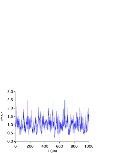
Figure 1: a quiet time series of the fluctuating plasma density normalized to its local mean value, with $R=30\%$ and $\tau_{c}=3$ $\mu$s, as for a typical plasma conditions near the LCFS.

By multiplying the denominator and the numerator in the right hand side of Eq. (8) by $\psi$, we obtain the new Pearson representation of the gamma process,

$$\dfrac{\partial P(\psi)}{\partial\psi}=\dfrac{(1-1/\nu)\psi-\psi^{2}/\left<\psi\right>}{\psi^{2}/\nu}P(\psi),$$ (11)

then the corresponding stochastic differential equation follows from Eq. (7),

$$\dfrac{\partial\psi}{\partial t}=\gamma\psi(t)-\dfrac{\psi^{2}(t)}{\left<\psi\right>\tau}+R\sqrt{2/\tau}\psi(t)w(t),$$ (12)

with $\gamma=(1+R^{2})/\tau$. In order to clarify the role of the time scale $\tau$, the dynamics of the correlation function $\rho(t)$ is required. It is straightforwardly derived from Eq. (12),

$$\dfrac{\partial\rho(t)}{\partial t}-\gamma\rho(t)=\dfrac{\gamma}{R^{2}}-\dfrac{1}{\tau R^{2}\left<\psi\right>^{3}}\left<\psi^{2}(t)\psi(0)\right>,$$ (13)

the term between brackets is a two-time correlation and can be approximated by,

$$\left<\psi^{2}(t)\psi(0)\right>=\eta\rho(t)+\kappa,$$ (14)

where the constant coefficients are fixed using the two particular cases $\tau_{c}=0$, $\rho(t)=0$ and $\tau_{c}=\infty$, $\rho(t)=1$. We get $\kappa=\left<\psi\right>\left<\psi^{2}\right>$ and $\eta=\left<\psi^{3}\right>-\left<\psi\right>\left<\psi^{2}\right>$. Then Eq. (13) reduces to,

$$\dfrac{\partial\rho(t)}{\partial t}+\gamma\rho(t)=0,$$ (15)

the correlation function is exponential $\rho(t)=\exp(-\gamma t)$, with $\tau_{c}=1/\gamma$ as a correlation time. Then $\tau=(1+R^{2})\tau_{c}$ is nothing but the correlation time increased by a factor $1+R^{2}$. It is worth noticing that the approximation Eq. (14) becomes exact in our case where $\psi$ is gamma distributed. This point is not developed here and can be demonstrated by writing $\psi$ as a square of Gaussian r.v. and using the Wick factorization theorem.
Equation (12) is the main result of this Letter. It is quadratically nonlinear and evolves on a turbulence correlation time scale. The process Eq. (12) has a consistent physical meaning, since the linear growth is driven by the fluctuations amplitude. As a response to this growth, a nonlinear damping takes place and is proportional to the fluctuation level $\psi(t)/\left<\psi\right>$. The dynamics is driven by a multiplicative white noise with variance $R^{2}$. This stochastic drift disappears and the dynamics evolves deterministically when the fluctuations amplitude vanishes ($R=0$). Unlike Eq. (1) which is based on the Gaussian assumption of the dynamical variable, and the process Eq. (4) obeying a linear stochastic differential equation, our stochastic model Eq. (12), shows how the gamma distribution and the associated universal $K$-$S$ scaling rise self-consistently from the quadratically nonlinear dynamics of the intermittent variable. Equation (12) behaves like the stochastic generalization of the L-H transient paradigm equation Bian (2010), with the difference that the latter is quadratic for the energy $E=((\psi-\left<\psi\right>)/\left<\psi\right>)^{2}$, leading to the Nakagami distribution for the plasma density.

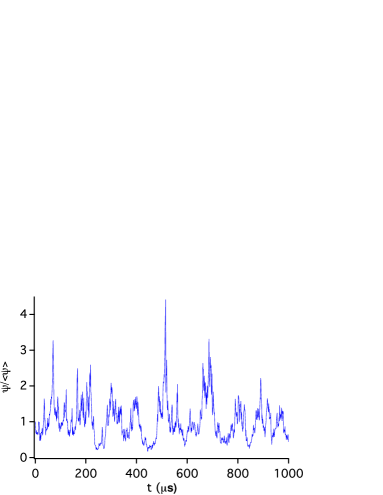
Figure 2: a weakly intermittent time series of the fluctuating plasma density normalized to its local mean value, with $R=50\%$ and $\tau_{c}=16$ $\mu$s, as for a typical plasma conditions of the near SOL.

Figure 3: a strongly intermittent time series of the fluctuating plasma density normalized to its local mean value, with $R=90\%$ and $\tau_{c}=55$ $\mu$s, as for a typical far SOL plasma conditions.

The stationary solution of Eq. (12) is the gamma distribution with stationary but not necessarily homogeneous parameters. Hence it can be used to analyze the nonlinear time series of the plasma density at different radial SOL positions $x$, using the local average field $\left<\psi\right>(x)$, correlation time $\tau_{c}(x)$ as well as $R(x)$. In order to simulate a plasma density time series in different conditions, we have used the Ito’s representation of Eq. (12) for the fluctuation level $\xi=\psi(t)/\left<\psi\right>$,

$$d\xi=\dfrac{\xi}{\tau_{c}}dt-\dfrac{\xi^{2}}{\tau_{c}(1+R^{2})}dt+R\sqrt{\dfrac{2}{\tau_{c}(1+R^{2})}}\xi dw(t).$$ (16)

In Fig. 1 is plotted a quiet time series of $\xi(t)$ with time step $dt=1$ $\mu$s, the fluctuations amplitude is of $R=30\%$ and the correlation time of $\tau_{c}=3$ $\mu$s, as in the typical edge plasma conditions close to the LCFS Graves et al. (2005). Fig. 2 gives another time series representative of an intermediate situation corresponding to the near SOL with moderate fluctuations amplitude $R=50\%$ and $\tau_{c}=16$ $\mu$s, tree bursts exceeding the average value by a factor of $3$ rise in the range of $1$ ms. A strongly intermittent time series is plotted in Fig. 3 with $R=90\%$ and $\tau_{c}=55$ $\mu$s, tree bursts exceeding $4\left<\psi\right>$ and a super burst with the amplitude of $10\left<\psi\right>$ are observed in the time range of $1$ ms, as is typically the case in the far SOL Sandberg et al. (2009).
In order to investigate the role of the nonlinear dynamics in the statistical characterization of intermittent fluctuations, we compare the gamma process to the existing stochastic models. The beta distribution has been used to fit the plasma density data in the edge of TORPEX, according to its capability to have negative skewness and its finite support Labit et al. (2007). Let consider here the standardized beta distribution,

$$P(\psi)\propto\psi^{\alpha-1}\left(1-\psi\right)^{\beta-1},\;0<\psi<1,\;\alpha,\;\beta>0,$$ (17)

where $\alpha=1/R^{2}-\left<\psi\right>(1+1/R^{2})$ and $\beta=\alpha(1/\left<\psi\right>-1)$. The beta distribution obeys the Pearson equation, then using Eq. (7), we derive the following stochastic differential equation,

$$\dfrac{\partial\psi}{\partial t}=\dfrac{\alpha+1}{\tau}\psi+\dfrac{\beta-\alpha-3}{\tau}\psi^{2}+\psi\sqrt{2\dfrac{1-\psi}{\tau}}w(t),$$ (18)

showing that the quadratically nonlinear dynamics of the beta process is systematically accompanied with a root square nonlinearity. Thus unlike the beta process, the gamma process and its stochastic representation Eq. (12) is in good agreement with the theoretical quadratic nonlinearity prediction and the experimental measurements. Indeed it has been pointed out that it is sufficient to fit the plasma density signals using a limiting beta distribution which coincides with the gamma PDF for positive skewness and using a shifted gamma r.v., $2\left<\psi\right>-\psi$, for negative skewness Labit et al. (2007). The comparison between the gamma and the beta processes shows the importance of the PDF functional form used to fit experimental data. With identical two first moments, different distributions (gamma, beta and log-normal) could provide a reasonable fit of experimental measurements, although the nonlinearity degrees of their dynamics is different. Therefore, and in order to improve the connection between the theory of nonlinear dynamics and the experimental time series, the analysis of plasma’s fluctuations using strong criteria Kagan et al. (1973); Lukacs (1955); McKenzie (1982) are suitable to clarify how long the statistics follows a given distribution. This procedure is preferable to the data fitting and a statistical signature based on the $K$-$S$ scaling, since no unicity exists between this scaling and the underlying distributions.
As a summary, we have derived a quadratically nonlinear stochastic differential equation for the intermittent plasma density in the SOL of fusion devices. The plasma density dynamics evolves on a turbulence correlation time scale ($\tau_{c}=1-100$ $\mu$s), and is characterized by the local fluctuations amplitude $R=10-90\%$. This equation is consistent with the experimental measurements and a theoretical prediction, since it behaves a gamma marginal and a quadratic nonlinearity. Its simple representation is suitable for edge plasma modeling, since a finite plasma density correlation time, together with high fluctuations amplitude affect considerably the plasma-wall interaction and the associated transport of sputtered impurities and released molecules Pigarov et al. (2011); Mekkaoui et al. (2012). The sensitivity of the nonlinearity degrees to the intermittent distribution has been investigated by comparing two potentially used distributions. Our result shows that the gamma distribution agrees with the quadratic nonlinearity, in comparison with the beta distribution leading to a root square nonlinearity.

References

- Carreras (2005) B. A. Carreras, J. Nucl. Mater. 337, 315 (2005).
- D’Ippolito et al. (2011) D. A. D’Ippolito, J. R. Myra, and S. J. Zweben, Phys. Plasmas 18, 060501 (2011).
- Krommes (2002) J. A. Krommes, Phys. Report 360, 1 (2002).
- Krommes (2008) J. A. Krommes, Phys. Plasmas 15, 030703 (2008).
- Lenschow et al. (1994) D. H. Lenschow, J. Mann, and L. Kristensen, J. Atmos. Ocean. Technol 11, 661 (1994).
- Sandberg et al. (2009) I. Sandberg, S. Benkadda, X. Garbet, G. Ropokis, K. Hizanidis, and del-Castillo-Negrete, Phys. Rev. Lett. 103, 165001 (2009).
- Graves et al. (2005) J. P. Graves, J. Horacek, R. A. Pitts, and K. I. Hopcraft, Plasma Phys. Controlled Fusion 47, L1 (2005).
- Labit et al. (2007) B. Labit, I. Furno, A. Fasoli, A. Diallo, S. H. Müller, G. Plyushchev, M. Podestà, and F. M. Poli, Phys. Rev. Lett. 98, 255002 (2007).
- Jakeman and Pusey (1978) E. Jakeman and P. N. Pusey, Phys. Rev. Lett. 40, 546 (1978).
- Garcia (2012) O. E. Garcia, Phys. Rev. Lett. 108, 265001 (2012).
- Rice (1944) S. O. Rice, Bell Syst. Tech. J. 23, 282 (1944).
- Brissaud and Frisch (1974) A. Brissaud and U. Frisch, J. Math. Phys. 15, 524 (1974).
- Jakeman (1980) E. Jakeman, J. Phys. A: Math. Gen. 13, 31 (1980).
- Gardiner (2009) C. Gardiner, Stochastic methods (Springer, 2009).
- Ozaki (1992) T. Ozaki, Statistica Sinica 2, 113 (1992).
- Cox et al. (1985) J. C. Cox, J. E. Ingersoll, and J. S. A. Ross, Econometrica 53, 385 (1985).
- Lamberton and Lapeyre (2000) D. Lamberton and B. Lapeyre, Stochastic Calculus Applied to Finance (Chapman & Hall/CRC, 2000).
- Bian (2010) N. H. Bian, Phys. Plasmas 17, 044501 (2010).
- Kagan et al. (1973) A. M. Kagan, Y. V. Linnik, and C. R. Rao, Characterization Problems in Mathematical Statistics (John Wiley & Sons, New York, 1973).
- Lukacs (1955) E. Lukacs, Ann. Math. Stat. 26, 319 (1955).
- McKenzie (1982) E. McKenzie, J. Appl. Prob. 19, 463 (1982).
- Pigarov et al. (2011) A. Y. Pigarov, S. I. Krasheninnikov, and T. D. Rognlien, Phys. Plasmas 18, 092503 (2011).
- Mekkaoui et al. (2012) A. Mekkaoui, Y. Marandet, D. Reiter, P. Boerner, P. Genesio, J. Rosato, R. Stamm, H. Capes, M. Koubiti, and L. Godbert-Mouret, Phys. Plasmas 19, 060701 (2012).