Hydrodynamic capabilities of an SPH code incorporating an artificial conductivity term with a gravity-based signal velocity

This paper investigates the hydrodynamic performances of an SPH code incorporating an artificial heat conductivity term in which the adopted signal velocity is applicable when gravity is present. To this end, we analyze results from simulations produced using a suite of standard hydrodynamical test problems. In accordance with previous findings it is shown that the performances of SPH to describe the development of Kelvin-Helmholtz instabilities depend strongly on the consistency of the initial condition set-up and on the leading error in the momentum equation due to incomplete kernel sampling. On the contrary, the presence of artificial conductivity does not significantly affect the results.

An error and stability analysis shows that the quartic $B-$spline kernel ($M_{5}$) possesses very good stability properties and we propose its use with a large neighbor number, between $\sim 50$ (2D) to $\sim 100$ (3D), to improve convergence in simulation results without being affected by the so-called clumping instability. Moreover, the results of the Sod shock tube test demonstrate that in order to obtain simulation profiles in accord with the analytic solution, for simulations employing kernels with a non-zero first derivative at the origin it is necessary the use of a much larger number of neighbors than in the case of the $M_{5}$ runs.

SPH simulations of the blob test show that in order to achieve blob disruption it is necessary the presence of an artificial conductivity term. However, it is found that in the regime of strong supersonic flows an appropriate limiting condition, which depends on the Prandtl number, must be imposed on the artificial conductivity SPH coefficients in order to avoid an unphysical amount of heat diffusion.

Results from hydrodynamic simulations that include self-gravity show profiles of hydrodynamic variables that are in much better agreement with those produced using mesh-based codes. In particular, the final levels of core entropies in cosmological simulations of galaxy clusters are consistent with those found using AMR codes. This demonstrate that the proposed diffusion scheme is capable of mimicking the process of entropy mixing which is produced during structure formation because of diffusion due to turbulence.

Finally, results of the Rayleigh-Taylor instability test demonstrate that in the regime of very subsonic flows the code has still several difficulties in the treatment of hydrodynamic instabilities. These problems being intrinsically due to the way in which in standard SPH gradients are calculated and not to the implementation of the artificial conductivity term. To overcome these difficulties several numerical schemes have been proposed which, if coupled with the SPH implementation presented in this paper, could solve the issues which recently have been addressed in investigating SPH performances to model subsonic turbulence.

1 INTRODUCTION

Smoothed particle hydrodynamics (SPH) is a Lagrangian, mesh-free, particle method which is used to model fluid hydrodynamics in numerical simulations. The technique was originally developed in an astrophysical context (Lucy 1977; Gingold & Monaghan 1977), but since then it has been widely applied in many other areas (Monaghan 2005) of computational fluid dynamics.

The method has several properties which make its use particularly advantageous in astrophysical problems (Hernquist & Katz 1989; Rosswog 2009; Springel 2010). Because of its Lagrangian nature the development of large matter concentrations in collapse problems is followed naturally, moreover the method is free of advection errors and is Galilean invariant, Finally, the method naturally incorporates self-gravity and possess very good conservation properties, its fluid equations being derived from variational principles.

The other computational fluid dynamical method commonly employed in numerical astrophysics is the standard Eulerian grid based approach in which the fluid is evolved on a discretized mesh (Stone & Norman 1992; Ryu et al. 1993; Norman & Bryan 1999b; Fryxell et al. 2000; Teyssier 2002). The spatial resolution of an Eulerian scheme based on a fixed Cartesian grid is often insufficient however to adequately resolve the large dynamic range frequently encountered in many astrophysical problems, such as galaxy formation. This has motivated the development of adaptative mesh refinement (AMR) methods, in which the spatial resolution of the grid is locally refined according to some selection criterion (Berger & Colella 1989; Kravtsov, Klypin & Khokhlov 1997; Norman 2005). Additionally, the order of the numerical scheme has been improved by adopting the parabolic piecewise method (PPM) of Colella & Woodward (1984), such as in the AMR Eulerian codes ENZO (Norman & Bryan 1999b) and FLASH (Fryxell et al. 2000).

Application of these different types of hydrodynamical codes to the same test problem with identical initial conditions should in principle lead to similar results. However, there has been growing evidence over recent years that in a variety of hydrodynamical test cases there are significant differences between the results produced the two types of methods (O’Shea et al. 2005a; Agertz et al. 2007; Wadsley, Veeravalli & Couchman 2008; Tasker et al. 2008; Mitchell et al. 2009; Read, Hayfield & Agertz 2010; Valcke et al. 2010; Junk et al. 2010).

For instance, Agertz et al. (2007) showed that in the standard SPH formulations the growth of Kelvin-Helmholtz (KH) instabilities in shear flows is artificially suppressed when steep density gradients are present at the contact discontinuities. Moreover, the level of central entropy produced in binary merger non-radiative simulations of galaxy clusters is significantly higher by a factor $\sim 2$ in Eulerian simulations than in those made using SPH codes (Mitchell et al. 2009). The origin of these discrepancies has been recognized (Agertz et al. 2007; Read, Hayfield & Agertz 2010) as partly due to the intrinsic difficulty for SPH to properly model density gradients across fluid interfaces, which in turn implies the presence of a surface tension effect which inhibits the growth of KH instabilities. A second problem is due to the Lagrangian nature of SPH codes, which prevents mixing of fluid elements at the particle level and leads to entropy generation (Wadsley, Veeravalli & Couchman 2008; Mitchell et al. 2009). In particular, Mitchell et al. (2009) argue that the main explanation for the different levels of central entropy found in cluster simulations is due to the different degree of entropy mixing present in the two codes. Unlike SPH, in Eulerian codes fluid mixing occurs by definition at the cell level and a certain degree of overmixing is certainly present in those simulations made using mesh-based codes (Springel 2010b).

Given the advantages of SPH codes highlighted previously, it appears worth pursuing any improvement in the SPH method capable of overcoming its present limitations. Along this line of investigation many efforts have been made by a number of authors (Abell 2011; Price 2008; Wadsley, Veeravalli & Couchman 2008; Valcke et al. 2010; Read, Hayfield & Agertz 2010; Heß & Springel 2010; Cha, Inutsuka & Nayakshin 2010; Murante et al. 2011).

Price (2008) introduces an artificial heat conduction term in the SPH equations with the purpose of smoothing thermal energy at fluid interfaces. This artificial conductivity (AC) term in turn gives a smooth entropy transition at contact discontinuities with the effect of enforcing pressure continuity and removing the artificial surface tension effect which inhibits the growth of KH instabilities at fluid interfaces. Similarly, Wadsley, Veeravalli & Couchman (2008) suggest that in SPH the lack of mixing at the particle level can be alleviated by adding a heat diffusion term to the equations so as to mimic the effects of subgrid turbulence, thereby improving the amount of mixing.

Read, Hayfield & Agertz (2010) present an SPH implementation in which a modified density estimate is adopted (Ritchie & Thomas 1991), together with the use of a peaked kernel and a much larger number of neighbors. The authors showed that the new scheme is capable of following the development of fluid instabilities in a better way than in standard SPH. Abell (2011) presents an alternative derivation of the SPH force equation which avoids the problem encountered by standard SPH in handling fluid instabilities, although the approach is not inherently energy or momentum conserving and is prone to large integration errors when the simulation resolution is low.

The method proposed by Inutsuka (2002) reformulates the SPH equations by introducing a kernel convolution so as to consistently calculate density and hydrodynamic forces. The latter are determined using a Riemann solver (Godunov SPH). The method has recently been revisited by Cha, Inutsuka & Nayakshin (2010) and Murante et al. (2011), who showed that the code correctly follows the development of fluid instabilities in a variety of hydrodynamic tests.

A deeper modification than those presented here so far has been introduced by Heß & Springel (2010), who replaced the traditional SPH kernel approach with an new density estimate based on Voronoi tesselation. The authors showed that the method is free of surface tension effects and therefore the growth rate of fluid instabilities is not adversely affected as in standard SPH.

Finally, a radically new numerical scheme has been introduced by Springel (2010b), with the purpose of retaining the advantages of both SPH and mesh-based codes. In the new code the hydrodynamic equations are solved on a moving unstructured mesh using a Godunov method with an exact Riemann solver. The mesh is defined by the Voronoi tesselation of a set of discrete points and is allowed to move freely with the fluid. The method is therefore adaptative in nature and thus Galilean invariant but, at the same time, the accuracy with which shocks and contact discontinuities are described is that of an Eulerian code. In a recent paper Bauer & Springel (2012) argue that the standard formulation of SPH fails to accurately resolve the development of turbulence in the subsonic regime (but see Price (2012b) for a different viewpoint). The authors draw their conclusions by analyzing results from simulations of driven subsonic turbulence made using the new moving-mesh code, named AREPO, and a standard SPH code.

Similar conclusions were reached in a set of companion papers (Sijacki et al. 2011; Vogelsberger et al. 2011), in which the new code was used in galaxy formation studies to demonstrate its superiority over standard SPH. However, the code is characterized by considerable complexity which makes the use the SPH scheme still appealing and, more generally, it is desirable that simulation results produced with a specific code should be reproduced with a completely independent numerical scheme when complex non-linear phenomena are involved. It appears worthwhile, therefore, to investigate, along the line of previous authors, the possibility of constructing a numerical scheme based on the traditional SPH formulation which is capable of correctly describing the development of fluid instabilities and at the same time incorporates the effects of self-gravity when present.

This is the aim of the present study, in which the SPH scheme is modified by incorporating into the equations an AC diffusion term as described by Price (2008). However, in Price (2008) the strength of the AC is governed by a signal velocity which is based on pressure discontinuities. For simulations where gravity is present this approach is not applicable because hydrostatic equilibrium requires pressure gradients. An appropriate signal velocity for conductivity when gravity is present is then used to construct an AC-SPH code with the purpose of treating the growth of fluid instabilities self-consistently. The viability of the approach is tested using a suite of test problems in which results obtained using the new code are contrasted with the corresponding ones produced in previous work using different schemes. The code is very similar in form to that presented by Wadsley, Veeravalli & Couchman (2008), but here the energy diffusion equation is implemented in a different manner.

The paper is organized as follows. Sect. 2 presents the hydrodynamical method and introduces the AC approach. In Sect. 3 we investigate the effectiveness of the method by presenting results from a suite of purely hydrodynamical test problems. These are: the two-dimensional Kelvin-Helmholtz instability, the Sod shock tube, the point explosion or Sedov blast wave test and the blob test. In Sect. 4 we then discuss results from hydrodynamic tests that include self-gravity. Specifically, we consider the cold gas sphere or Evrard collapse test, the Rayleigh-Taylor instability and the cosmological integration of galaxy clusters. Finally, the main results are summarized in Sect. 5

2 The Hydrodynamic method

Here we present the basic features of the method, for recent reviews see Rosswog (2009), Springel (2010) and Price (2012).

2.1 Basic SPH equations

In the SPH method the fluid is described by a set of $N$ particles with mass $m_{i}$, velocity $\@vec{v}_{i}$, density $\rho_{i}$, and a thermodynamic variable such as the specific thermal energy $u_{i}$ or the entropic function $A_{i}$. The particle pressure is then defined as $P_{i}=(\gamma-1)\rho_{i}u_{i}=A_{i}\rho_{i}^{\gamma}$, where $\gamma=5/3$ for a monoatomic gas. The density estimate $\rho(\@vec{r})$ at the particle position $\@vec{r}_{i}$ is given by

$$\rho_{i}=\sum_{j}m_{j}W(|\@vec{r}_{ij}|,h_{i})\leavevmode\nobreak\ ,$$ (1)

where $\@vec{r}_{ij}\equiv\@vec{r}_{i}-\@vec{r}_{j}$, $W(|\@vec{r}_{ij}|,h_{i})$ is the interpolating kernel that has compact support and is zero for $|\@vec{r}_{ij}|\geq\zeta h_{i}$ (Price 2012). The kernel is normalized to the condition $\int Wd^{D}r=1$. The sum in Eq. (1) is over a finite number of particles and the smoothing length $h_{i}$ is a variable that is implicitly defined by the equation

$$f_{D}(\zeta h_{i})^{D}\rho_{i}=N_{sph}m_{i}\leavevmode\nobreak\ ,$$ (2)

where $D$ is the number of spatial dimensions, $f_{D}=\pi,4\pi/3$ for $D=2,3$ and $N_{sph}$ is the number of neighboring particles within a radius $\zeta h_{i}$ . This equation can be rewritten by defining $h_{i}$ in units of the mean interparticle separation

$$h_{i}=\eta(m_{i}/\rho_{i})^{1/D}\leavevmode\nobreak\ ,$$ (3)

so that $N^{2D}_{sph}={\pi(\zeta\eta)^{2}}$ and $N^{3D}_{sph}={4\pi(\zeta\eta)^{3}}/{3}$. The smoothing length $h_{i}$ is determined by solving the non-linear equation (2); note that $N_{sph}$ does not necessarily need to be an integer but can take arbitrary values if $\eta$ is used as the fundamental parameter determining $h_{i}$ (Price 2012). A kernel commonly employed is the $M_{4}$, or cubic spline, which is zero for $\zeta\geq 2$. In three dimensions typical choices for $N_{sph}$ lie in the range $N_{sph}\sim 33-64$, which for the $M_{4}$ kernel corresponds to $\eta\simeq 1.-1.25$. The equation of motion for the SPH particles can be derived from the Lagrangian of the system (Springel 2010; Price 2012) and is given by

$$\frac{d\@vec{v}_{i}}{dt}=-\sum_{j}m_{j}\left[\frac{P_{i}}{\Omega_{i}\rho_{i}^{2}}\@vec{\nabla}_{i}W_{ij}(h_{i})+\frac{P_{j}}{\Omega_{j}\rho_{j}^{2}}\@vec{\nabla}_{i}W_{ij}(h_{j})\right]\leavevmode\nobreak\ ,$$ (4)

where the coefficients $\Omega_{i}$ are defined as

$$\Omega_{i}=\left[1-\frac{\partial h_{i}}{\partial\rho_{i}}\sum_{k}m_{k}\frac{\partial W_{ik}(h_{i})}{\partial h_{i}}\right].$$ (5)

These terms are present in the momentum equation (4) because the smoothing length $h_{i}$ itself is implicitly a function of the particle coordinates through Eq. (2).

2.2 Artificial viscosity

In SPH, the momentum equation must be generalized by adding an appropriate viscous force, which is aimed at correctly treating the effects of shocks. An artificial viscosity (AV) term is then introduced with the purpose of dissipating local velocities and preventing particle interpenetration at the shock locations. The new term is given by

$$\left(\frac{d\@vec{v}_{i}}{dt}\right)_{AV}=-\sum_{i}m_{j}\Pi_{ij}\@vec{\nabla}_{i}\bar{W}_{ij}\leavevmode\nobreak\ ,$$ (6)

where the term $\bar{W}_{ij}=\frac{1}{2}(W(r_{ij},h_{i})+W(r_{ij},h_{j}))$ is the symmetrized kernel and $\Pi_{ij}$ is the AV tensor. In the SPH entropy formulation (Springel & Hernquist 2002), it is the entropy function per particle $A_{i}$ which is integrated and its time derivative is calculated as follows

$$\frac{dA_{i}}{dt}=\frac{1}{2}\frac{\gamma-1}{\rho_{i}^{\gamma-1}}\sum_{j}m_{j}\Pi_{ij}\@vec{v}_{ij}\cdot\nabla_{i}\bar{W}_{ij}\equiv\frac{\gamma-1}{\rho_{i}^{\gamma-1}}\left(\frac{du_{i}}{dt}\right)_{AV}\leavevmode\nobreak\ ,$$ (7)

where $\@vec{v}_{ij}=\@vec{v}_{i}-\@vec{v}_{j}$. For the AV tensor we adopt here the form proposed by (Monaghan 1997) in analogy with Riemann solvers:

$$\Pi_{ij}=-\frac{\alpha_{ij}}{2}\frac{v^{AV}_{ij}\mu_{ij}}{\rho_{ij}}f_{ij}\leavevmode\nobreak\ ,$$ (8)

where

$$v^{AV}_{ij}=c_{i}+c_{j}-3\mu_{ij}$$ (9)

is the signal velocity and $\mu_{ij}=\@vec{v}_{ij}\cdot\@vec{r}_{ij}/|r_{ij}|$ if $\@vec{v}_{ij}\cdot\@vec{r}_{ij}<0$ but zero otherwise, so that $\Pi_{ij}$ is non-zero only for approaching particles. Here scalar quantities with the subscripts $i$ and $j$ denote arithmetic averages, $c_{i}$ is the sound speed of particle $i$, the parameter $\alpha_{i}$ regulates the amount of AV, and $f_{i}$ is a controlling factor that reduces the strength of AV in the presence of shear flows. The latter is given by (Balsara 1995)

$$f_{i}=\frac{|\@vec{\nabla}\cdot\@vec{v}|_{i}}{|\@vec{\nabla}\cdot\@vec{v}|_{i}+|\@vec{\nabla}\times\@vec{v}|_{i}}\leavevmode\nobreak\ ,$$ (10)

where $(\@vec{\nabla}\cdot\@vec{v})_{i}$ and $(\@vec{\nabla}\times\@vec{v})_{i}$ are the standard SPH estimates for divergence and curl (Monaghan 2005). For pure shear flows $|\@vec{\nabla}\times\@vec{v}|_{i}>>|\@vec{\nabla}\cdot\@vec{v}|_{i}$ so that the AV is strongly damped.

Using the signal velocity (9), the Courant condition on the timestep of particle $i$ reads

$$\Delta t^{C}_{i}\simeq 0.3\frac{h_{i}}{max_{j}|v^{AV}_{ij}|}.$$ (11)

In the standard SPH formulation the viscosity parameter $\alpha_{i}$ which controls the strength of the AV is given by $\alpha_{i}=\mathrm{const}\equiv\alpha_{0}$, with $\alpha_{0}=1$ being a common choice (Monaghan 2005). This scheme has the disadvantage that it generates viscous dissipation in regions of the flow that are not undergoing shocks. In order to reduce spurious viscosity effects Morris & Monaghan (1997) proposed making the viscous coefficient $\alpha_{i}$ time dependent so that it can evolve in time under certain local conditions. The authors proposed an equation of the form

$$\frac{d\alpha_{i}}{dt}=-\frac{\alpha_{i}-\alpha_{min}}{\tau_{i}}+{S}_{i}\leavevmode\nobreak\ ,$$ (12)

where ${S}_{i}$ is a source term and $\tau_{i}$ regulates the decay of $\alpha_{i}$ to the floor value $\alpha_{min}$ away from shocks. For the source term the following expression is adopted

$${S}_{i}=S_{0}f_{i}(-(\@vec{\nabla}\cdot\@vec{v})_{i},0)(\alpha_{max}-\alpha_{i})\leavevmode\nobreak\ ,$$ (13)

which is constructed in such a way that it increases in the presence of shocks. The prefactor $S_{0}$ is unity for $\gamma=5/3$ and the damping factor $f_{i}$ is inserted to account for the presence of vorticity. The original form proposed by Morris & Monaghan (1997) has been refined by the factor $(\alpha_{max}-\alpha_{i})$ (Rosswog et al. 2000), which has the advantage of being more sensitive to shocks than the original formulation and of preventing $\alpha_{i}$ from becoming higher than a prescribed value $\alpha_{max}$. Recently, Cullen & Dehnen (2011) presented an improved version of the Morris & Monaghan (1997) AV scheme, employing as shock indicator a switch based on the time derivative of the velocity divergence.

The decay parameter $\tau_{i}$ is of the form

$$\tau_{i}=\frac{h_{i}}{c_{i}\leavevmode\nobreak\ l_{d}}\leavevmode\nobreak\ ,$$ (14)

where $l_{d}$ is a dimensionless parameter which controls the decay time scale. In a number of test simulations, (Rosswog et al. 2000) found that appropriate values for the parameters $\alpha_{max},\alpha_{min}$, and $l_{d}$ are $1.5,0.05$, and $0.2$, respectively. In principle, the effects of numerical viscosity in regions away from shocks can be reduced by setting $l_{d}$ to higher values than $l_{d}=0.2$. In practice, the minimum time necessary to propagate through the resolution length $h_{i}$ sets the upper limit $l_{d}=1$. However, the time evolution of the viscosity parameter can be affected if very short damping timescales are imposed. Neglecting variations in the coefficients, the solution to Eq. (12) at times $t>t_{in}$ can be written as

$$\alpha_{i}(t)=q_{i}+(\alpha_{i}(t_{in})-q_{i})\exp^{-(t-t_{in})/\tau^{\prime}_{i}}\leavevmode\nobreak\ ,$$ (15)

where

$$\tau^{\prime}_{i}=\frac{\tau_{i}}{1+S_{i}\tau_{i}}\leavevmode\nobreak\ ,$$ (16)

and $q_{i}$ is a modified source term

$$q_{i}=\frac{\alpha_{min}+S_{i}\tau_{i}\alpha_{max}}{1+S_{i}\tau_{i}}.$$ (17)

From Eq. (15) it can be seen that $\alpha_{i}(t)\simeq\alpha_{max}$ in the strong shock regime $S_{i}\tau_{i}\gg 1$ but this condition is not satisfied if $S_{i}\tau_{i}\lower 2.15277pt\hbox{$\;\buildrel<\over{\sim}\;$}1$. Therefore for mild shocks this implies that, if very short decay time scales are imposed, the peak value of $\alpha_{i}(t)$ at the shock front might be below the AV strength necessary to properly treat shocks.

To overcome this difficulty a modification to (13) has been adopted (Valdarnini 2011, herefater V11) which, when $l_{d}=1$, compensates the smaller values of $S_{i}\tau_{i}$ with respect to the small $l_{d}$ regimes. This is equivalent to considering a higher value for $\alpha_{max}$, so that in Eq. (13) $\alpha_{max}$ is substituted by $\alpha_{max}\rightarrow\xi\alpha_{max}$.

Table 1: KH parameters for the simulations. From top to bottom: simulation label, Mach number $M$ and $x-$velocity $v_{1}$ of the high-density layer, KH time scale $\tau_{KH}$

label run	1	2	3	4	5
M	0.2	0.4	0.6	0.8	1.0
$|v_{x}|$	0.26	0.52	0.77	1.0	1.3
$\tau_{KH}$	1.23	0.56	0.37	0.28	0.22

The correction factor $\xi$ has been calibrated using the shock tube problem as reference and requiring a peak value of $\sim 0.6-0.7$ for the viscosity parameter at the shock front, as in the $l_{d}=0.2$ case. The results indicate that a normalization of the form $\xi=(l_{d}/0.2)^{0.8}$ for $l_{d}\geq 0.2$ satisfies these constraints. This normalization has been validated in a number of other test problems showing that it is able to produce a peak value of the viscosity parameter at the shock location which is independent of the chosen value of the decay parameter $l_{d}$.

The time-dependent AV formulation of SPH has been shown to be effective in reducing the damping of turbulence due to the effects of numerical viscosity in simulations of galaxy clusters (Dolag et al. 2005, V11) Moreover, it has been used in a recent paper (Price 2012b) to argue that the conclusion of Bauer & Springel (2012) about the difficulty for SPH codes in properly modeling the development of subsonic turbulence is based just on using a SPH code in its standard AV formulation. In the following, unless otherwise stated, simulations will be performed using a time-dependent AV; this will be fully specified by the set of parameters $\{\alpha_{min},\alpha_{max},l_{d}\}$.

2.3 Artificial conductivity

As already outlined in the Introduction, different formulations have been proposed for overcoming the problems encountered by standard SPH in the treatment of fluid discontinuities. Here we follow the approach suggested by Price (2008), who proposed adding a dissipative term to the thermal energy equation for smoothing the energy across contact discontinuities. The presence of these dissipative terms introduces a smoothing of entropy at fluid interfaces with the effect of removing pressure discontinuities.

The motivations lying at the basis of this approach were discussed by Monaghan (1997), who showed how the momentum and energy equations in SPH must contain a dissipative term related to jumps in the variables across characteristics, in analogy with the corresponding Riemann solutions.

The artificial conductivity (AC) term for the dissipation of energy takes the form

$$\left(\frac{du_{i}}{dt}\right)_{AC}=\sum_{j}\frac{m_{j}v^{AC}_{ij}}{\rho_{ij}}\left[\alpha^{C}_{ij}(u_{i}-u_{j})\right]\@vec{e_{ij}}\cdot\@vec{\nabla_{i}}\bar{W}_{ij}\leavevmode\nobreak\ ,$$ (18)

where $v^{AC}_{ij}$ is the signal velocity, which does not need to be the same as that used in the momentum equation, $\@vec{e}_{ij}\equiv\@vec{r}_{ij}/r_{ij}$ and $\alpha^{C}_{i}$ is the AC parameter which is of order unity . Eq. (18) represents the SPH analogue of a diffusion equation of the form

$$\left(\frac{du_{i}}{dt}\right)_{AC}\simeq D^{AC}_{i}\nabla^{2}u_{i}\leavevmode\nobreak\ ,$$ (19)

where

$$\nabla^{2}u_{i}=2\sum_{j}m_{j}\frac{u_{i}-u_{j}}{\rho_{j}}\frac{\@vec{e}_{ij}\cdot\@vec{\nabla}W_{ij}}{r_{ij}}$$ (20)

is the SPH expression for the Laplacian (Brookshaw 1985) and, in analogy with the analysis of Lodato & Price (2010) for defining an equivalent physical viscosity coefficient for the SPH numerical viscosity, we can define $D^{AC}_{i}$ as a numerical heat diffusion coefficient given by

$$D^{AC}_{i}\simeq\frac{1}{2}\alpha^{C}_{i}v^{AC}_{ij}r_{ij}\leavevmode\nobreak\ .$$ (21)

Table 2: Main simulation parameters of the KH tests. From top to bottom: simulation label, kernel function, neighbor number, signal velocity used in Eq. (18), setup of initial HCP lattice: U=unsmoothed, S=smoothed. For all of the runs the AV parameters are $\{\alpha_{min},\alpha_{max},l_{d}\}=\{0.1,1.5,1\}$.

Simulations	SPH	RHO	LIQ	LP	CRT	M5
Kernel	CS	CS	LIQ	LIQ	CRT	M5
$N_{s}$	32	32	32	32	32	50
$v^{sig}$	grav	grav	grav	pres	grav	grav
$\rho$	U	S	S	S	S	S

An important issue concerns the choice of the AC parameter $\alpha^{C}_{i}$ which must be constructed so that diffusion of thermal energy is kept under control and is damped away from discontinuities. This can be achieved by introducing a switch similar to that devised for AV. The dissipation parameter is then evolved according to

$$\frac{d\alpha^{C}_{i}}{dt}=-\frac{\alpha^{C}_{i}-\alpha^{C}_{min}}{\tau^{C}_{i}}+{S^{C}}_{i}\leavevmode\nobreak\ ,$$ (22)

the meaning of the terms being similar to that of Eq. (12). In particular, for the decay timescale $\tau^{C}_{i}={h_{i}}/{\mathcal{C}c_{i}}$ we set here $\mathcal{C}=0.2$ and set to zero the floor value $\alpha^{C}_{min}$. For the source term $S^{C}_{i}$ the following expression is used

$${S^{C}}_{i}=f_{C}h_{i}\frac{|\nabla^{2}u_{i}|}{\sqrt{u_{i}+\varepsilon}}(\alpha^{C}_{max}-\alpha^{C}_{i})\leavevmode\nobreak\ ,$$ (23)

where $f_{C}$ is a dimensionless parameter of order unity and the parameter $\varepsilon$ avoids divergences as $u_{i}\rightarrow 0$. This equation differs from the corresponding source term proposed by Price & Monaghan (2005), Price (2008) by the factor $\alpha^{C}_{max}-\alpha^{C}_{i}$ which has been inserted here in analogy with Eq. (13) for introducing a stronger response of the switch in the presence of discontinuities. The choice of values for the parameters $f_{C}$ and $\alpha^{C}_{max}$ depends on the problem under consideration, for example Price & Monaghan (2005) proposed $f_{C}=0.1$. Here a number of numerical experiments has shown that the best results in terms of response of the AC parameter $\alpha^{C}_{i}$ to the presence of discontinuities are obtained by setting $f_{C}=1$ and $\alpha^{C}_{max}=1.5$, which we assume henceforth as reference values. Moreover it is found that significant benefits in terms of sharpness of the AC parameter profile across the discontinuity are obtained by inserting the $\alpha^{C}_{max}-\alpha^{C}_{i}$ term. In principle, the choice of the derivative term used to detect discontinuities is arbitrary, but in practice a second derivative (Price & Monaghan 2005) term ensures better sensitivity to sharp discontinuities in thermal energy than a first derivative (Price 2005a).

An example of a signal velocity specifically designed to remove pressure gradients at contact discontinuities is that originally introduced by Price (2008) for pure hydrodynamical simulations

$$v^{AC}_{ij}(P)=\sqrt{\frac{|P_{i}-P_{j}|}{\rho_{ij}}}\leavevmode\nobreak\ ,$$ (24)

and further refined by Valcke et al. (2010). The ability of the new AC formulation of SPH to follow the development of KH instabilities using this expression for the signal velocity has been verified in a number of tests (Price 2008; Valcke et al. 2010; Merlin et al. 2010). However, the disadvantage of the signal speed (24) is that it cannot be applied when self-gravity is considered because in that case a pressure gradient is present at hydrostatic equilibrium. Imagine, for example, a self-gravitating gas sphere in hydrostatic equilibrium in which there is a negative radial temperature gradient, with the gas temperature decreasing when moving outward from the center of the sphere. An application of the SPH equations, with the AC term of Eq. (22) now using the signal velocity (24), will lead to a heat flux from the inner to the outer regions and, in the long term, to the development of an unphysical isothermal temperature profile. A signal velocity which avoids this difficulty is given by

$$v^{AC}_{ij}(grav)=|(\@vec{v}_{i}-\@vec{v}_{j})\cdot\@vec{r}_{ij}|/r_{ij}\leavevmode\nobreak\ ,$$ (25)

which corresponds to the formulation proposed by Wadsley, Veeravalli & Couchman (2008) in which a dissipative term is added to the evolution of the thermal equation with the purpose of modeling heat diffusion due to turbulence. The new term is constructed in analogy with the subgrid-scale model of Smagorinsky (1963) and is given by

$$\left(\frac{du_{i}}{dt}\right)_{AC}=C\sum_{j}\frac{m_{j}|\@vec{v}_{i}-\@vec{v}_{j}|(h_{i}+h_{j})}{\rho_{ij}}(u_{i}-u_{j})\@vec{e}_{ij}\cdot\@vec{\nabla_{i}}\bar{W}_{ij}\leavevmode\nobreak\ ,$$ (26)

where $C$ is a coefficient of order unity, whose precise value depends on the problem under consideration. For the rising hot bubble problem considered by Wadsley, Veeravalli & Couchman (2008), the best agreement with the corresponding PPM results taken as reference is obtained setting $C=0.1$, higher values being too much diffusive. Throughout this paper the SPH simulations of the hydrodynamic tests are performed by adopting the expression (18) for the thermal energy dissipative term. With respect to the formulation of Wadsley, Veeravalli & Couchman (2008) this approach presents the advantage of using a diffusion parameter which is not constant but evolves in time according to a source term, so that the amount of diffusion away from discontinuities is minimized. For the AC signal velocity, we then use expression (25), whose performances in the AC formulation (18) has not been fully tested before in SPH simulations of hydrodynamic test problems.

Note that, using the signal velocity (25), the Von Neumann stability criterion becomes unimportant with respect the Courant condition (11). The Von Neumann constraint requires $\Delta t\leq 0.5\Delta x^{2}/D$, which in SPH reads

$$\Delta t_{i}^{AC}\lower 2.15277pt\hbox{$\;\buildrel<\over{\sim}\;$}\frac{1}{2}\frac{h^{2}_{i}}{D_{i}^{AC}}\leavevmode\nobreak\ .$$ (27)

Since $\alpha^{C}\simeq O(1)$, this condition implies $\Delta t_{i}^{AC}\lower 2.15277pt\hbox{$\;\buildrel>\over{\sim}\;$}\Delta t_{i}^{C}$ in both the supersonic and subsonic regimes.

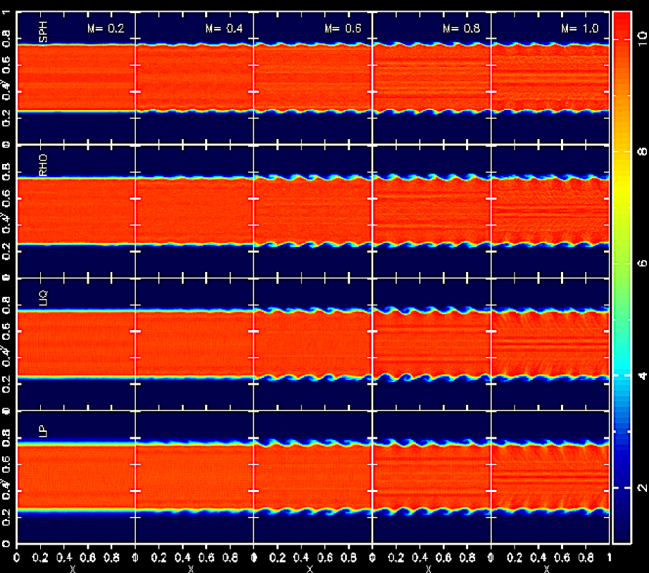
Figure 1: Density maps for some of the 2D KH instability tests described in Sect. 3.1. From left to right, each column shows the panels for runs having initial conditions with the same Mach number at the corresponding time $t=\tau_{KH}$, as listed in Table 1. From top to bottom, different rows refer to the following simulations : SPH, RHO, LIQ and LP. The latter use the linear quartic kernel but with the signal velocity (24), whereas the first three use the expression (25) (see Table 2). The plots can be compared directly with Fig. 10 of Valcke et al. (2010).

3 Hydrodynamic tests

In the following, simulation results obtained by applying the new AC-SPH code to a number of hydrodynamic test problems are discussed with the objective of validating the code and assessing its performance. To this end, the simulation results of the tests will be compared with the corresponding ones obtained by previous authors using different codes and/or numerical methods. The problems considered are usually presented in the literature in dimensional or complexity order, but here we follow a different approach. Since the KH instability is the hydrodynamic test which initially (Agertz et al. 2007) originated the discussion about the difficulties of standard SPH in properly handling the development of instabilities, and it is also the most widely considered in this context (Abell 2011; Price 2008; Cha, Inutsuka & Nayakshin 2010; Heß & Springel 2010; Read, Hayfield & Agertz 2010; Valcke et al. 2010; Murante et al. 2011), we here discuss first in detail the two-dimensional version of the test. The setup of the other runs will then be considered in the light of the results obtained from the 2D KH test.

3.1 2D Kelvin-Helmholtz instability

The KH instability arises in the presence of shear flow between two fluid layers when a small velocity perturbation is imposed in the direction perpendicular to the interface between the two fluids. The development of the instability is characterized by an initial phase, where the fluids interpenetrate each other, and then the forming of vortices, which become progressively more pronounced and turn into KH rolls at the onset of non-linearity. In the case of incompressible fluids for a sinusoidal perturbation of wavelength $\lambda$, this phase is reached with a time-scale (Chandrasekhar 1961)

$$\tau_{KH}=\frac{\lambda(\rho_{1}+\rho_{2})}{\left(\rho_{1}\rho_{2}\right)^{1/2}v}\leavevmode\nobreak\ ,$$ (28)

where $\rho_{1}$ and $\rho_{2}$ are the fluid densities and $v=v_{1}-v_{2}$ is the relative shear velocity. A proper modeling of instabilities in numerical hydrodynamics is essential since the KH instability plays a crucial role in the development of turbulence which occurs in many hydrodynamical phenomena. In particular, the KH instability is relevant in many astrophysical processes, such as gas stripping from cold gas clouds occurring in galactic haloes and the production of entropy in the intracluster gas of galaxy clusters due to injection of turbulence.

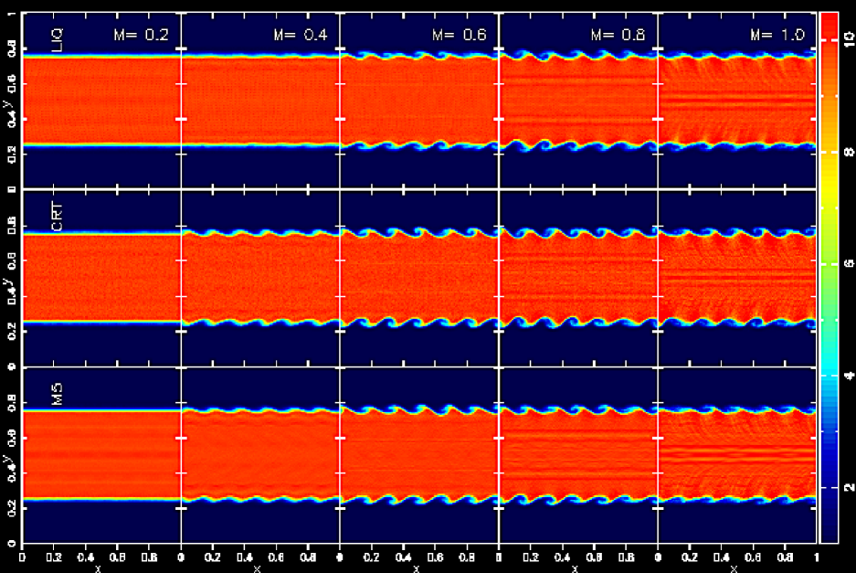
Figure 2: As in Fig. 1 but for the set of simulations LIQ, CRT and $M_{5}$.

The growth of the KH instability in hydrodynamic simulations has been addressed by various authors (Abell 2011; Price 2008; Wadsley, Veeravalli & Couchman 2008; Read, Hayfield & Agertz 2010; Valcke et al. 2010; Heß & Springel 2010; Cha, Inutsuka & Nayakshin 2010; Murante et al. 2011). These studies found that the development of the instability is artificially suppressed because of two distinct effects: the first problem is the so-called local mixing instability (LMI) which is due to entropy conservation and which inhibits mixing at the kernel scale thus introducing pressure discontinuities; the second problem arises because of errors in the momentum equation which cannot be reduced by increasing the number of neighbor particles without causing particle clumping.

Given the wide variety of numerical parameters and initial conditions with which the KH instability has been addressed, we choose here to perform the tests using as reference the simulations presented by Valcke et al. (2010). In particular, the authors implement in their SPH equations an AC term as that of Eq. (18), but with the AC parameter set to unity, and with a signal velocity given by Eq. (24). The authors performed a systematic analysis of the capabilities of SPH to capture the KH instability using different SPH formulations, kernels, numerical resolutions and KH time-scales. This choice allows to assess code capabilities by constructing a large suite of simulations whose numerical results can be contrasted against the corresponding ones discussed by Valcke et al. (2010).

3.1.1 Initial conditions set-up

The problem domain consists of a periodic box of unit length with cartesian coordinates $x\in\{0,1\}$, $y\in\{0,1\}$. Within the domain there is a fluid with adiabatic index $\gamma=5/3$ which satisfies the following conditions:

$$\rho,\leavevmode\nobreak\ T,v_{x}=\left\{\begin{array}[]{ l l }\rho_{1},T_{1},v_{1}&|y-0.5|\leq 0.25\\ \rho_{2},T_{2},v_{2}&|y-0.5|>0.25.\end{array}\right.$$ (29)

As in Valcke et al. (2010), we choose here $\rho_{1}=10$ and $\rho_{2}=1$, with the index $1$ referring to the high density layer. This choice is motivated by the finding that the difficulties of SPH in reproducing KH instabilities increase as the density contrast between the two fluid layers gets higher. The two layers are in pressure equilibrium with $P_{1}=P_{2}=10$ so that the sound velocities in the two layers are $c_{1}=\sqrt{{\gamma P_{1}}/{\rho_{1}}}=1.29$ and $c_{2}=\sqrt{{\gamma P_{2}}/{\rho_{2}}}=4.08$ , respectively. The layers slide against each other with opposite shearing velocities $v_{1}=-v_{2}$ and in order to seed the KH instability a small single-mode velocity perturbation is imposed along the $y-$direction

$$v_{y}=w_{0}\sin(2\pi x/\lambda)\leavevmode\nobreak\ ,$$ (30)

where $w_{0}=0.025$ and $\lambda=1/6$. In order to restrict the perturbation to spatial regions in the proximity of the interfaces, the perturbation (30) is applied only if $|y-\sigma|<0.025$, where $\sigma$ takes the values of $0.25$ and $0.75$, respectively. With this choice of parameters, the Mach number of the high-density layer is $M\simeq v_{1}/c_{1}\simeq v_{1}/1.29$ and the KH time-scale is $\tau_{KH}\simeq 0.29/v_{1}$. As in Valcke et al. (2010), we consider KH simulations with a range of five different Mach numbers; Table 1 reports the values of $M$ together with the respective values of $v_{1}$ and $\tau_{KH}$.

In order to implement the the density set-up (29), a two-dimensional lattice of equal mass particles is placed inside the simulation box. We adopt here an isotropic hexagonal-close-packed (HCP) configuration for the particles coordinates instead of the more commonly employed Cartesian grid. The advantage of this configuration is that, for a given number of neighbors, it gives a better density estimate due to its symmetry properties. To construct the initial density configuration (29), the lattice spacing of the particles is varied until the SPH density estimate (1) satisfies the required values within a certain tolerance criterion ($\lower 2.15277pt\hbox{$\;\buildrel<\over{\sim}\;$}1\%$) for the relative density error. The simulations were run using a total number of $N=512^{2}$ particles and the initial particle specific energies were assigned after the density calculation so as to satisfy pressure equilibrium. This particle number is larger than that used in the runs of Valcke et al. (2010) ($\simeq 200K$), but guarantees a density setup with the specified tolerance criterion.

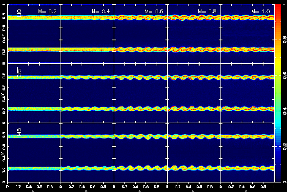
Figure 3: Rendered plots of the $\alpha^{C}$ parameters are shown for the same runs as in Fig. 2. The distribution of particle values $\alpha^{C}_{i}$ has been interpolated at the map grid points according to the SPH prescription.

As noticed by Valcke et al. (2010) and other authors, SPH is a numerical method which can only represent smoothed quantities, and so applying it to hydrodynamic problems where strong density gradients are present can lead to inconsistencies. This is, in fact, the situation encountered by standard SPH in the treatment of KH instabilities, where the lack of entropy mixing induces an artificial pressure discontinuity at fluid interfaces with a jump in density.

Motivated by these difficulties, we consider here a set of runs in which the density discontinuity at the interfaces is replaced by a smooth transition. To allow making a consistent comparison with the corresponding runs of Valcke et al. (2010), we adopt the same smoothing profile

$$\rho(y)=D\pm A\mathrm{atan}\left[B(y^{\prime}+C)\right]\leavevmode\nobreak\ ,$$ (31)

where the coefficients are given by

$$A=\frac{\rho_{1}-\rho_{2}}{2\mathrm{atan}(\beta)}\leavevmode\nobreak\ ,$$ (32)

$$B=2\frac{\beta}{\delta}\leavevmode\nobreak\ ,$$ (33)

$$C=-\frac{\delta}{2}\leavevmode\nobreak\ ,$$ (34)

$$D=\frac{\rho_{1}+\rho_{2}}{2}\leavevmode\nobreak\ ,$$ (35)

and $y^{\prime}=y-\sigma+\delta/2$. In Eq. (31) the sign in front of the coefficient $A$ refers to $\sigma=0.25,\leavevmode\nobreak\ 0.75$ respectively. The parameters $\beta$ and $\delta$ determine the thickness of the density transition and take the values $\beta=10$, $\delta=0.5/0.75$.

Figure 4: As in Figures 1 and 2 but here at the time $t=2$ for all of the panels. Note from Table 1 that this implies $t>>\tau_{KH}$ for runs with high Mach number.

The following procedure is adopted in order to construct a lattice configuration which satisfies the density profile given by Eq. (31). An HCP lattice of particle is first constructed in the domain $0\leq x<1$ and $0\leq y\leq 0.5$ with a spacing $a_{down}$ such that the SPH density is $\rho=\rho_{2}$. Proceeding upward from $y=0$, the lattice spacing is progressively reduced according to $a=a_{down}[\rho_{2}/\rho(y)]^{1/2}$ until $y=0.25$ and $N_{down}$ particles are left. The same procedure is applied to a high-density lattice which in the same domain satisfies the condition $\rho=\rho_{1}$: starting from $y=0.5$ and proceeding downward, the lattice spacing is increased so that $a=a_{up}[\rho_{1}/\rho(y)]^{1/2}$ until $y=0.25$ and $N_{up}$ particles remain of the original high-density lattice. The whole procedure is numerically iterated until the numbers $N_{down}$ and $N_{up}$ satisfy the conditions $N_{down}+N_{up}=N/2$ and $N_{up}/N_{down}=\rho_{1}/\rho_{2}$. The lattice is then replicated in the top half of the box ($y\rightarrow 1-y$) so that the initial conditions are fully symmetric around $y=0.5$. In the following, simulations with initial conditions for which the particle positions are arranged in a unsmoothed HCP lattice are denoted with the suffix SPH, whereas all of the others adopt the smoothed density profile constructed according to the procedure described here.

Another issue which is found to have a significant impact on the ability of standard SPH to properly capture KH instabilities is the choice of the kernel function. According to Read, Hayfield & Agertz (2010), the accuracy of the momentum equation for particle $i$ is governed by the leading error

$$\@vec{E_{i}}^{0}=\sum_{j}\frac{m_{j}}{\rho_{j}}\left[\frac{\rho_{i}}{\rho_{j}}+\frac{\rho_{j}}{\rho_{i}}\right]h_{i}\@vec{\nabla}_{i}\bar{W}_{ij}\leavevmode\nobreak\ ,$$ (36)

which vanishes in the continuum limit. However, this does not hold for a finite number of irregularly distributed particles or, more specifically, in the proximity of a contact discontinuity where a density step is present. A possible solution consists of increasing the number of neighbors so as to improve kernel sampling, although this approach presents some difficulties when the commonly employed $M_{4}$ or cubic spline (CS) SPH kernel is used. This occurs because for a large number of neighbors the CS kernel is subject to the so-called clumping instability, in which pairs of particles with interparticle distance $q=r/h<2/3$ remain close together because the CS kernel gradient tends to zero below this threshold distance. A stability analysis (Morris 1996; Børve, Omang & Trulsen 2004; Price 2005a; Read, Hayfield & Agertz 2010) shows that for the CS kernel, a Cartesian lattice of particles is unstable for $\eta\simeq 1.5$ or $N_{sph}\sim 28,110$ when $D=2$ and $D=3$, respectively. The clumping degrades the spatial resolution because it reduces the effective number of neighbors with which integrals are sampled, thus still having large $\@vec{E}_{0}$ errors even when the resolution is increased. To overcome this problem one can modify the kernel shape in order to have a non-zero kernel derivative at the origin. However, for a fixed number of neighbors, kernels of this kind have the drawback of giving a less accurate density estimate than that given by the CS kernel since near the origin the kernels have a steeper profile.

As an alternative to the CS kernel, we consider here the linear quartic (LIQ) kernel, introduced by Valcke et al. (2010), which is a quartic polynomial for $q_{s}\leq q\leq\zeta=2$ and is linear for $0\leq q<q_{s}$. The choice of the parameter $q_{s}$ determines the quality of density estimates. From a set of 2D Sod shock tube runs, Valcke et al. (2010) recommend $q_{s}=0.6$, which is the value adopted here. For the functional form and normalization of the kernel see Valcke et al. (2010).

Another kernel which has been introduced for the purpose of avoiding particle clumping is the core triangle (CRT) kernel (Read, Hayfield & Agertz 2010) which has constant first derivative for $0\leq q<\alpha$ and is similar to the CS kernel for $\alpha\leq q\leq\zeta=2$. This kernel is of the form

$$w(q)=\frac{\sigma}{h^{D}}\left\{\begin{array}[]{ll}\left(-3\alpha+\frac{9}{4}\alpha^{2}\right)q+1+\frac{3}{2}\alpha^{2}-\frac{3}{2}\alpha^{3}&0\leq q<\alpha;\\ 1-\frac{3}{2}q^{2}+\frac{3}{4}q^{3}&\alpha\leq q<1;\\ \frac{1}{4}\left(2-q\right)^{3},&1\leq q<2;\\ 0.&q\geq 2,\end{array}\right.$$ (37)

where $1/\sigma=2\pi{\left(\frac{7}{20}+\frac{\alpha^{4}}{8}-\frac{3}{20}\alpha^{5}\right)},\leavevmode\nobreak\ 4\pi\left(\frac{1}{4}+\frac{\alpha^{5}}{20}-\frac{\alpha^{6}}{16}\right)$ for $D=2$ and $D=3$ , respectively. The value of $\alpha$ is fixed by the condition of continuity for the second derivative, giving $\alpha=2/3$. For the grid of initial conditions previously described, the sample of KH simulations is then constructed by performing SPH runs with the same initial conditions but using different kernels. We consider the CS kernel, together with the LIQ and CRT kernels. For all of these runs the number of neighbors is $N_{sph}=32\leavevmode\nobreak\ (\eta\simeq 1.5)$.

However, another solution for reducing sampling errors consists of still keeping a $B-$spline kernel function but increasing its order (Price 2012, sect.5.4). This approach presents the advantage of retaining the bell shape of the kernel, a feature which provides good density estimates (Fulk & Quinn 1996). After the $M_{4}$ (CS) kernel, at the next order is the $M_{5}$ or quartic kernel

$$w(q)=\frac{\sigma}{h^{D}}\left\{\begin{array}[]{ll}\left(\frac{5}{2}-q\right)^{4}-5\left(\frac{3}{2}-q\right)^{4}+10\left(\frac{1}{2}-q\right)^{4},&0\leq q<\frac{1}{2};\\ \left(\frac{5}{2}-q\right)^{4}-5\left(\frac{3}{2}-q\right)^{4},&\frac{1}{2}\leq q<\frac{3}{2};\\ \left(\frac{5}{2}-q\right)^{4},&\frac{3}{2}\leq q<\frac{5}{2};\\ 0.&q\geq\frac{5}{2},\end{array}\right.$$ (38)

which is truncated to zero for $\zeta\geq 2.5$ and has $\sigma={96}/{1199\pi},{1}/{20\pi}$ for $D=2$ and $D=3$, respectively.

An additional set of SPH simulations was then performed using the $M_{5}$ spline as the kernel. For consistency with the other runs, we kept the same ratio of smoothing length to particle spacing ($\eta\sim 1.5$) so that for these runs the chosen number of neighbors is $N_{sph}=50$. A non trivial issue concerns the role of pairing instability for this class of kernels. Because the gradient of the $M_{5}$ kernel still goes to zero as $q\rightarrow 0$, one would expect the instability still to occur for $\eta\sim 1.5$. Nonetheless, it will be seen that KH simulations with the $M_{5}$ kernel do not exhibit particle clumping, in contrast with corresponding simulations performed with the CS kernel. This suggests that the stability properties of the $M_{5}$ kernel are better than those of the CS one; this topic will be discussed in a subsequent dedicated section (3.1.3).

Table 2 summarizes the main simulation parameters used in the KH tests. For comparison purposes, a set of mirror runs was carried out for the LIQ simulations in which Eq. (25), for the signal velocity, was replaced in Eq. (18) by Eq. (24) which is based on pressure discontinuities.

3.1.2 Results

Fig. 1 shows the density maps at $t=\tau_{KH}$ for some of the KH simulations listed in Table 2. The panels can be compared directly with the corresponding ones in Fig. 10 of Valcke et al. (2010). A visual inspection reveals that the expected features of the KH runs are correctly reproduced and of a general consistency between the results produced by the two codes. In particular, the LP simulations which use the pressure-based AC signal velocities (24) appear to produce results almost identical to the corresponding LIQ ones. Thus showing how, for the KH tests examined here, the use of the two signal velocities can be considered equivalent, within the spanned range of Mach numbers.

Note, however, the absence of KH rolls for the LP run with $M=0.4$, whereas for the same simulation in Valcke et al. (2010) the rolls have already been developed. Given the general agreement between the two codes it is hard to ascertain the origin of the discrepancy for this specific run. However, the panels of Fig. 1 show that the AC-SPH formulation, and this point will be discussed in detail later in sect. 4.2, is still unable to properly capture the development of KH instabilities for very subsonic shear flows. This suggests how small differences in the time integration procedure of the two codes can become manifest in the long-term evolution of cold flows.

In Fig. 2 the results for the same set of KH simulations of Table 1 are shown, but with the use of kernels LIQ, CRT and $M_{5}$. An important feature is now the appearance for the CRT and $M_{5}$ runs of KH rolls in the $M=0.4$ case. This improvement in the description of KH instabilities suggests that integration errors, that are present with the LIQ kernel, are now absent or reduced in the CRT and $M_{5}$ runs. However, in the $M=0.2$ case, the kernels are still unable to capture the development of the KH instability. For this test case, a high-resolution run ($N=1024^{2}$) using the $M_{5}$ kernel (not shown here) still reveals the absence of any KH roll at $t=\tau_{KH}$, thus showing that in SPH the problem of an accurate description of KH instabilities in the very subsonic regimes is not a resolution issue or due to the AC implementation. See also McNally, Lyra & Passy (2011) for a recent discussion on this topic.

To test the effectiveness of the switch (13) in ensuring a fast response of the $\alpha_{i}^{C}$ parameters to the presence of thermal energy discontinuities, Fig. 3 renders the plots of the AC parameters that are shown for the test runs of Fig. 2. The maps are color coded according to the range of values of $\alpha_{i}^{C}$. The highest values lie in the range $\sim 0.7-0.8$ and are confined in a narrow strip around the interface layers, with the floor value $\sim 0$ as the background value away from the discontinuities. Note that in general, and in particular for the $M=1$ test case, the maximum values of the $\alpha^{C}$ for the $M_{5}$ runs are below those of the other runs. A result due to a faster growth rate of the instability, ensured by an improved kernel accuracy in interpolating the variables.

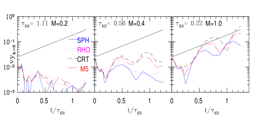
Figure 5: Time evolution of the velocity field amplitude in the $y$ direction, as measured by the $k\lambda=12\pi$ mode of the Fourier transform of $v_{y}$, for some of the KH instability tests described in Sect. 3.1. Each panel refers to KH simulations performed with the same Mach number, the initial conditions set-up being given in Table 1. Within each panel, the different curves are for AC-SPH runs with different simulation parameters, as specified in Table 2. The black solid line indicates the expected linear theory growth rate.

The long term evolution of the KH tests is shown at $t=2$ in Fig. 4. The overall features of the density plots for different runs are similar to their counterparts displayed in Fig. 11 of Valcke et al. (2010). Note the tendency for the $M_{5}$ runs to the appearance of small scale features at the layer contacts.

The aim of this section is to test the consistency of the present AC implementation by comparing results, extracted from a suite of AC-SPH simulations of the 2D KH instability problem, with those of similar runs (Valcke et al. 2010). The results of the KH tests indicate a code behavior which is in accord with what expected and with the simulations of Valcke et al. (2010).

However, Valcke et al. (2010) argue that it is not the absence of the AC term the main reason of the SPH failure to develop KH instabilities, although the presence of AC is necessary for the long-term evolution of the instabilities, but this difficulty of SPH is rather due to two distinct reasons. The first issue is a general problem of consistency of the initial condition set-up, as SPH by definition can only deal with smoothed quantities and therefore its application to problems where sharp discontinuities are present leads to inconsistencies. This is part of the more general problem (Robertson et al. 2010) of properly smoothing in numerical simulations of hydrodynamic test problems the discontinuities initially present at the interfaces, so to achieve convergence in the solution. This aspect of the KH test problem can be cured by properly stretching the initial particle lattice so as to introduce a smooth density transition at the interfaces. The results indicate a significant improvement in the capability of SPH to properly capture the correct growth rate of the KH instability.

The other issue which causes a poor performance of SPH when handling KH instabilities is the leading error in the momentum equation due to incomplete kernel sampling. This error can be reduced by removing particle clumping, which depends on the kernel stability properties. In fact, the kernels LIQ and CRT have been introduced (Read, Hayfield & Agertz 2010; Valcke et al. 2010) with the aim of removing the clumping instability. Since the results of the simulations suggest performances for the $M_{5}$ kernel that are quite similar to those achieved by these kernels, it is therefore interesting to better quantify the relative performances of these kernels.

Following Junk et al. (2010), we then measure the growth rate of the KH instability for some of the runs and compare it with the linear theory growth rate expectation $\propto e^{t/\tau_{KH}}$. This is achieved, using Fourier transforms, by measuring the time-evolution of the $\lambda=1/6$ growing mode of the $v_{y}$ velocity perturbation component. The details of the procedure are given in Junk et al. (2010) and will not be reported here. For the sake of clarity, the results of the LIQ runs are not displayed since they are quite similar to those of the CRT simulations. Moreover, we only display the growth rates for three different KH test cases, those with Mach number $M=0.2,0.4$ and $M=1$, the results of the others being intermediate between these.

There are a number of distinct features which are apparent from the panels of Fig. 5. The first is that simulations with smoothed IC ( RHO) perform systematically better than the unsmoothed ones (SPH). The second is that only for $M=1$ the simulations with kernels CRT and $M_{5}$ are able to correctly recover the expected growth rate. Finally, this capability degrades progressively as one considers lower Mach numbers. While this behavior is in accordance with the visual impression of the maps previously displayed, and confirms that the present SPH implementation still has problems in the description of instabilities in subsonic flows, it is interesting to note that the performances of the $M_{5}$ runs are similar to those obtained using the CRT kernel. This behavior is particularly interesting, since the simulations have been performed setting the ratio of the smoothing lengths to particle spacing to $\eta\simeq 1.5$ so that the pairing instability, that is present in the runs which use the CS kernel, should be present in the $M_{5}$ simulations as well.

How the clumping instability affects sampling errors can be assessed by computing the particle errors $\@vec{E}_{i}^{0}$, according to Eq. (36). The distribution, throughout the simulation domain of the $\@vec{E}_{i}^{0}$ errors versus $y$, is shown in the top panels of Fig. 6 for those $M=1$ simulations performed using different kernels. The solid lines represent the mean of the binned distributions. Similar plots have been produced by Valcke et al. (2010) and their Fig. 3 can be used for comparative purposes.

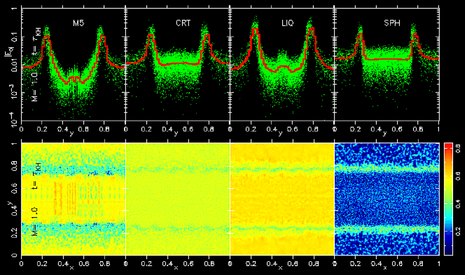
Figure 6: Top panels: distribution at time $t=\tau_{KH}$ of the errors $|\@vec{E_{i}}^{0}|$ plotted versus $y$, as defined by Eq. (36), for the KH runs with Mach number $M=1$ and different simulation parameters (See Table 2). The red histograms show the mean values of the binned distributions. Bottom panels: each panel shows the nearest neighbor map of the run in the corresponding top panel. This is defined as the distribution, interpolated at the map grid points of the normalized distances $q_{i}^{2}=\delta_{i}^{2}/h_{i}$, where $\delta_{i}^{k}$ is the distance $|\@vec{x}_{i}-\@vec{x}_{k}|$ of the $k-$th neighbor of the particle $i$ and the neighbors are sorted so that $\delta_{i}^{k}<\delta_{i}^{k+1}$ .

As expected, the largest $\@vec{E}^{0}$ errors are present in the SPH simulation, whereas better results are obtained by using the LIQ and CRT kernels, as indicated by the error distribution in their respective panels. This is a result of the absence of particle clumping for these simulations, owing to the specific stability properties of these kernels (Read, Hayfield & Agertz 2010; Valcke et al. 2010).

A striking feature is given vice versa by the $\@vec{E}^{0}$ error distribution of the simulation performed using the $M_{5}$ kernel, which, in fact, shows how the magnitude of the $\@vec{E}^{0}$ errors are even smaller than those of the two runs CRT and LIQ for this kernel. A result which is in accordance with what has been found previously by analyzing the growth rates, suggesting that, since all of the simulations were performed using the same $\eta$, the stability properties of the $M_{5}$ kernel are better than those of the CS one.

To further investigate this point, the bottom panels of Fig. 6 show the ‘nearest neighbor’ map of the corresponding top panels. This is defined by interpolating the quantity $q_{i}^{2}$ at the grid points, according to the SPH prescription, where for the $k-th$ neighbor $q_{i}^{k}=|\@vec{x}_{i}-\@vec{x}_{k}|/h_{i}$ and the neighbors have been sorted according to their distance from the particle $i$ itself.

The map of the $M_{5}$ kernel indicates a distribution of the second nearest neighbor distribution $q_{i}^{2}$ that is quite similar to that displayed by the CRT and LIQ kernels. The only difference being at the layer interfaces where the distribution of quantities $q_{i}^{2}$ for the $M_{5}$ kernel is slightly shifted towards smaller values than for the other kernels. Note, vice versa, how for the CS kernel because of the pairing instability, the distribution of the neighboring distances is flipped with respect that of the other kernels.

The results of Fig. 6, however, clearly show the absence of clumping instability for the $M_{5}$ kernel. In the next section, we investigate, in more detail, the stability properties of this kernel.

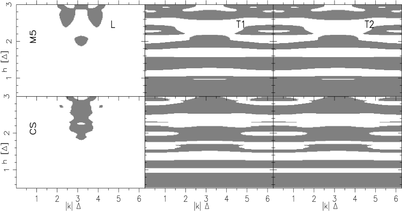
Figure 7: Contour plots of the dispersion relation (3.1.3) are shown as a function of wavenumber $k$ and smoothing length $h$ for a regular lattice of particles with spacing $\Delta$, we consider a wavevector with orientation $\@vec{k}=k(1,0,0)$. Gray areas indicate the instability regions for which $\omega^{2}<0$. From the left to right, the top panels show in the case of the $M_{5}$ kernel the instability regions of the longitudinal and the two transverse waves. The bottom panels refer to the CS ($M_{4}$) kernel.

3.1.3 Stability issues

The stability properties of SPH have been investigated by a number of authors (Swegle & Hicks 1995; Morris 1996; Monaghan 2000; Børve, Omang & Trulsen 2004; Read, Hayfield & Agertz 2010; Dehnen & Aly 2012). The instabilities are studied analytically by analyzing the dispersion relation for sound waves of small amplitude, propagating in a uniform medium. We now derive the dispersion relation for the SPH equation of motion in a manner similar to the analysis of previous authors. A uniform lattice of equal mass particles of mass $m$, density $\rho_{0}$, pressure $P_{0}$ and sound speed $c_{s}^{2}=\gamma P_{0}/\rho_{0}$ is perturbed by a small wave

$$\@vec{x_{i}}=\@vec{x_{i}}^{0}+\@vec{a}\exp[\@vec{k}\cdot\@vec{x_{i}}^{0}-\omega t]\leavevmode\nobreak\ ,$$ (39)

where $\@vec{a}$ is the perturbation, $\@vec{k}$ the wavevector and $\@vec{x_{i}}^{0}$ are the unperturbed particle positions. By linearizing the equation of motion for the perturbation one has the dispersion relation

$$\omega^{2}a_{\mu}=\left[\frac{2mP_{0}}{\rho^{2}_{0}}\sum_{j}H_{\mu\nu}(1-cos(\@vec{k}\cdot\@vec{x_{ij}}^{0})a_{\nu}+\right.$$

$$\mbox{}+\left.(\gamma-2)\frac{m^{2}P_{0}}{\rho_{0}^{3}}(\@vec{a}\cdot\@vec{q}^{i})q^{i}_{\mu}\right]\leavevmode\nobreak\ ,$$

where the summations are over the neighbors $j$ of particle $i$, the vector $\@vec{q}_{i}$ is defined as

$$\@vec{q_{i}}=\sum_{j}\sin\@vec{k}\cdot\@vec{x_{ij}}^{0}\@vec{\nabla}_{i}W_{ij}\leavevmode\nobreak\ ,$$ (40)

and ${\bf H}(W)$ is the Hessian of the kernel

$$H_{\mu\nu}=\frac{\partial^{2}W(r)}{\partial x_{\mu}\partial x_{\nu}}.$$ (41)

For a given smoothing length $h$ and wavevector $\@vec{k}$, the stable solutions of Eq. (3.1.3) are defined by the condition $\omega^{2}\geq 0$ . Solutions for which $\omega^{2}<0$ represent exponentially growing or decaying perturbations. Moreover, it is useful to define a numerical sound speed $C^{2}_{num}=\omega^{2}/k^{2}$ and a scaled numerical sound speed $c^{2}_{num}=C^{2}_{num}/c^{2}_{s}$. Clearly, the condition $c^{2}_{num}=1$ should be satisfied to correctly model the sound speed.

We now examine the stability properties of the CS and $M_{5}$ kernels. For simplicity, we consider a plane wave propagating along the $x-$axis, $\@vec{k}=k(1,0,0)$, and assume $\gamma=5/3$. The bottom panels of Fig 7 show, for the longitudinal and the two transverse waves of the perturbation, the instability regions of the CS kernel, these are denoted by the gray areas and represent the solutions to Eq. (3.1.3) , in the domain $(h,k)$, for which $\omega^{2}<0$. Similarly, the top panels are for the $M_{5}$ kernel.

The longitudinal wave perturbation is responsible for the clumping instability, whereas the traverse waves give rise to the so-called banding instability (Read, Hayfield & Agertz 2010). Unlike the clumping instability, the latter is relatively unimportant in causing sampling errors (Read, Hayfield & Agertz 2010) and will not be further considered here. A comparison of the two stability plots for the longitudinal wave solution clearly shows that the stability properties of the $M_{5}$ kernel are much better than those of the CS one.

This is part of a more general result which was already recognized by (Morris 1996): the stability properties of SPH are improved, as higher order spline kernels are used in place of the CS kernel. This occurs, basically, because the higher the order of the spline, the better it approximates a Gaussian kernel. In Eq. (3.1.3) one can see that the numerical sound speed $c^{2}_{num}$ depends on the first and second derivative of kernel $W$. Ideally, one should have $c^{2}_{num}\simeq 1$ to accurately describe the sound wave propagation and this condition is fulfilled as smoother kernels are used, so as to keep the numerical dependency of $c^{2}_{num}$ as weak as possible.

Note however that here, differently from the stability properties of the CRT kernel, the clumping instability is not entirely suppressed but rather it is present whenever $\eta\lower 2.15277pt\hbox{$\;\buildrel>\over{\sim}\;$}2.5$.

Finally, it must be stressed that the paring instability that occurs in the hydrodynamic tests described here, is unlikely to have a significant impact on many astrophysical problems of interest, where very cold flows are absent. Rasio & Lombardi (1999) estimate for instance, from SPH simulations of a stationary fluid, that lattice effects become important when velocity dispersions are below $\sim 3\%-4\%$ the sound speed.

The results of this section and of the previous one, therefore, suggest that in order to avoid the pairing instability, the $M_{5}$ kernel can be considered a viable alternative to the use of the otherwise steeper CRT and LIQ kernels, provided that the parameter $\eta$ is consistently rescaled. In the next section, we then discuss the related performances of these kernels in a test simulation.

3.2 Sod’s shock tube

A classic test used to investigate the hydrodynamic capabilities of SPH codes is the Sod shock tube problem (Hernquist & Katz 1989; Wadsley, Stadel & Quinn 2004; Springel 2005; Price 2008; Tasker et al. 2008; Rosswog 2009). This test consists in a fluid, initially at rest, in which a membrane located at $x=0$ separates the fluid on the right, with high density and pressure, from the fluid on the left, with lower density and pressure. The membrane is removed at $t=0$ and a shock wave develops propagating toward the left, followed by a contact discontinuity and a rarefaction wave propagating to the right.

A well known problem of standard SPH codes in reproducing the analytic solution of the shock tube problem is the presence of a pressure discontinuity that arises across the propagating contact discontinuity. Simulations incorporating an artificial thermal conductivity term in the SPH equations (Price 2008; Rosswog 2009; Price 2012) show shock profiles in which density and thermal energy are resolved across the discontinuity, hence giving a continuous pressure profile. However, in these runs the AC formulation adopts the AC signal velocity (24) where jumps in thermal energy are smoothed in accordance with the presence of pressure discontinuities. This is in contrast with the AC signal velocity (25) employed here, for which in absence of shear flows, contact discontinuities are unaffected and therefore cannot be used to remove the blip seen at the contact discontinuity in the pressure profile of the shock tube SPH runs.

However, the application of the AC-SPH code to this test is nonetheless of interest because it can still be used to validate code performances. In particular, we consider a 3D setup of the shock tube test and with these initial conditions we construct a set of AC-SPH simulations performed with different kernels and neighbor numbers. Shock tube profiles extracted from these simulations are compared with the aim of assessing the goodness of different kernels in reproducing, for a given test problem, profiles of known analytic solutions.

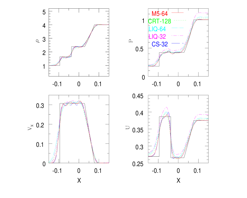
Figure 8: Results at $t=0.12$ of the 3D shock tube test. The profiles of: density, pressure, thermal energy and velocity are plotted clockwise from top left. The solid black line represents the analytical solution, while lines with different styles and colors are the profiles of the AC-SPH runs with different kernels and neighbor numbers, as illustrated in the pressure panel.

The initial condition setup consists of an ideal fluid with $\gamma=5/3$, initially at rest at $t=0$. An interface set at the origin separates the fluid on the right with density and pressure $(\rho_{1},P_{1})=(4,1)$ from the fluid on the left with $(\rho_{2},P_{2})=(1,0.1795)$. To construct these initial conditions, a cubic box of side-length unity was filled with $10^{6}$ equal mass particles, so that $800,000$ were placed in the right-half of the cube and $200,000$ in the left-half. The particles were extracted from two independent uniform glass-like distributions contained in a unit box consisting of $1.6\cdot 10^{6}$ and $4\cdot 10^{5}$ particles, respectively. This initial condition setup is the same previously implemented in Sect. 5.1 of V11, to test the time-dependent AV scheme described in Sect. 2.2.

For the same initial setup, to investigate the performances of different kernels in reproducing the analytic profiles of the shock tube problem, we perform runs with different kernels and neighbor numbers. The kernels considered are : CS, LIQ, CRT and $M5$. The number of neighbors varies in power of two between $32$ and $128$. The SPH runs were realized by imposing periodic boundary conditions along the $y$ and $z$ axes and the results were examined at $t=0.12$. We show results obtained using the standard AV formulation, the results of the other runs being unimportant from the viewpoint of kernel performances.

Some of the simulation profiles extracted from the 3D SPH runs of the shock tube test are shown in Fig. 8. A striking feature is the wide scatter between the pressure profiles of the runs performed using different kernels or neighbor numbers. The same behavior is present for the thermal energy profiles, whilst very similar density profiles are exhibited by the same runs.

There are several conclusions that can be drawn from the results of Fig. 8. The performances of the $M_{5}$-64 run are quite similar to those of CS-32, although for the former simulation a closer inspection reveals a slightly better treatment of the thermal energy spike at the contact discontinuity, the spike being due to the initial condition set-up.

The worst results are obtained by the LIQ simulations when using $N_{sph}=32$ or $N_{sph}=64$ neighbors. The profiles of the LIQ-128 run are not shown here to avoid overcrowding in the plots, and are quite similar to those of simulation CRT-128. This clearly demonstrates the need for this class of kernels to use a large ( say $\lower 2.15277pt\hbox{$\;\buildrel>\over{\sim}\;$}128$ ) number of neighbors, so as to compensate for the density underestimate due to the steeper profiles introduced to avoid the pairing instability.

To better quantify this density bias, Table  3 reports, for different kernels and neighbor number, the mean SPH density estimated from a glass-like configuration of $N=10^{6}$ particles, in a unit periodic box of total mass one. The results illustrate how the density estimate of the $M_{5}$ kernel with 64 neighbors is comparable to the CS one obtained using 32 neighbors, the value of $\eta$ being the same ($\eta\simeq 1$). Vice versa, for the LIQ and CRT kernels, only when $N_{sph}=128$ does the mean density approach the $M_{5}$-64 estimate.

The density values given in Table  3 also help to explain the rather poor performances of the LIQ kernel when using 32 neighbors. From Fig. 8 it can be seen that for the corresponding run the relative pressure error is $\varepsilon_{P}\simeq 10\%$ in the unperturbed right zone of the cube. This error is already present in the pressure profile at $t=0$ and it is originated from the density error due to the adopted kernel and neighbor number, together with the use of an entropy-conserving code to perform the simulations. Initially, particle entropies are assigned according to the initial conditions so that, for particles satisfying $x_{i}>0$, $A_{i}\equiv A_{1}=P_{1}/\rho_{1}^{\gamma}\simeq 0.1$. During the integration particle pressures are calculated according to $P_{i}=A_{i}\rho_{i}^{\gamma}$, and for $x>0$ a relative pressure error $\varepsilon_{P}\simeq\gamma\varepsilon_{\rho}\simeq 10\%$ is present when $\varepsilon_{\rho}\simeq 6\%$.

Taken at face value, the results of Table  3 demonstrate that in 3D simulations a conservative lower limit for the kernels with a modified shape, should be to assume at least $N_{sph}\lower 2.15277pt\hbox{$\;\buildrel>\over{\sim}\;$}200$ neighbors. In fact, in a recent paper Read & Hayfield (2012) presented a new formulation of SPH where they adopted, as reference, the so-called high-order core triangle (HOCT, Price (2005a)). The profile of this kernel is a generalization of that of the CRT kernel and the authors assume $N_{sph}=442$ as the reference value for their scheme.

However, the results of the previous sections suggest that the stability properties of the $M_{5}$ kernel can be profitably used, with an appropriate choice of the $\eta$ parameter, to avoid the pairing instability when dealing with tests of hydrodynamic instabilities in which cold flows are present.

Finally, the density estimates of Table  3 suggest that great care should be used when deciding on the goodness of a particular kernel on the basis of its relative performances in terms of density estimates. The results of the 3D Sod shock tube clearly indicate how there could be a large difference between the simulation and the expected solution profile of some hydrodynamic variable, such as pressure or thermal energy, while having, at the same time, a much smaller difference in the corresponding density profile.

3.3 Sedov blast wave

The Sedov blast wave test is used to validate, in three dimensions, the code capability in the strong shock regime. The test consists of a certain amount of energy $E$ which is injected at $t=0$ into a very small volume of an ambient medium of uniform density $\rho$. The spherically symmetric shock propagates outward from the initial volume and at the time $t$ the shock front is located at the radius (Sedov 1959)

$$R(t)\simeq\beta(Et^{2}/\rho)^{1/5}\leavevmode\nobreak\ ,$$ (42)

where $\beta\sim 1.15$ for $\gamma=5/3$.

Previous investigations (Rosswog & Price 2007; Merlin et al. 2010) showed that, owing to the large discontinuities initially present in the thermal energy, incorporating an artificial conduction term in the energy equation greatly improves the description of the shock front in the simulations. Without the presence of this term, the initially large discontinuity in the thermal energy will soon give rise to a disordered particle distribution thus degrading the shock profile (Rosswog & Price 2007).

The initial setting of the test is realized as follows. A HCP lattice of $N=2\cdot 64^{3}$ equal mass particles is arranged in a cubic box of side length unity. The particle masses are chosen so as to give $\rho=1$ and periodic boundary conditions are imposed. The nearest particle to the position $\{0.5,0.5,0.5\}$ is chosen as the center particle. In order to consistently represent a point-like explosion with the given numerical resolution, the particles $j$ comprised within the kernel radius $\zeta h_{i}$ of the center particle $i$ are given an initial thermal energy such that the total injected energy is $E=1$. This blast wave energy is distributed among the neighboring particles not uniformly but with a weight proportional to $W_{ij}$.

Table 3: Average densities and sample standard deviations estimated from the SPH densities of a configuration of one million particles. These are arranged in a glass-like configuration inside a cubic periodic box of side length unity and total mass one. The SPH particle densities have been calculated for a variety of kernels and neighbor numbers $N_{sph}$ (see text).

	$N_{sph}$
Kernel	$32$	$64$	$128$
CS	1.005 $\pm$ 0.035	1.002 $\pm$ 0.019	1.0018 $\pm$ 0.012
LIQ	1.06 $\pm$ 0.028	1.024 $\pm$ 0.016	1.01 $\pm$ 0.011
CRT	1.079 $\pm$ 0.039	1.035 $\pm$ 0.020	1.016 $\pm$ 0.012
M5	1.022 $\pm$ 0.052	1.003 $\pm$ 0.024	1.0008 $\pm$ 0.015

Using this initial condition set-up, we ran three test simulations, which differ in the choice of the adopted kernel and neighbor number. For the CS kernel, we use $N_{sph}=64$ neighbors. We also run two other test cases, now using the CRT and $M_{5}$ kernel and $N_{sph}=128$ neighbors. All of the simulations were performed using the implemented AC scheme and the time-dependent AV formulation with parameters given by $\{\alpha_{min},\alpha_{max},l_{d}\}=\{0.1,1.5,0.2\}$ .

Fig. 9 shows the radial density profiles at $t=0.06$ for the different test runs. The solid black line represents the expected analytic solution, with the shock front being located at $r\simeq 0.37$. Radial simulation profiles were obtained by averaging, for each radial bin $r_{k}$, SPH densities calculated from the particle distributions over a set of $(\theta,\phi)=(20,20)$ grid points uniformly spaced in angular coordinates: these are located at the surface of a sphere with radius $r_{k}$. The radial spacing is not uniform but is chosen so as to guarantee an accurate sampling of density in the proximity of the shock front, with about $\sim 40$ radial bins between $r\sim 0.34$ and $r\sim 0.42$.

All of the simulations are in fair agreement with the analytical solution and the differences between the simulation profiles are negligible. At the shock front, the profiles exhibit a density jump of about $\sim 2$, whereas the analytical solution gives a compression factor of $\gamma+1/\gamma-1=4$. These results are in accordance with previous findings (Rosswog & Price 2007; Springel 2010b; Heß & Springel 2010) and indicate that for 3D SPH simulations of the Sedov-Taylor point explosion problem the simulation profiles converge to the analytical solution as the resolution is increased, with approximately $\sim 345^{3}$ particles (Rosswog & Price 2007) being required to fully resolve the shock front.

Fig. 9 can also be used to verify the behavior of the individual time-step algorithm. For problems involving very strong shocks, as demonstrated by Saitoh & Makino (2009), individual particle time-steps must be properly restricted so to avoid that in the proximity of the shock front they do not satisfy the local Courant condition, thus leading to inaccuracies in the integration. In fact, SPH simulations using individual time-steps, but without an appropriate limiter, will fail to predict the expected solution profile (see Fig. 3 of Saitoh & Makino (2009)). The profiles of Fig. 9 demonstrate the correctness of the algorithm used to update the time-steps, although different from that devised by Saitoh & Makino (2009).

The present scheme adopts individual particle time-steps $\Delta t_{i}$ that can vary in power-of-two subdivisions of the largest allowed time-step $\Delta t_{0}\geq\Delta t_{i}$ (Hernquist & Katz 1989). At each step, particles whose time bin is synchronized with the current time are defined as ‘active’ and their hydrodynamic quantities, as well as their smoothing lengths and densities are consistently updated. However, non-active particles $j$, that are neighbors of an active particle $i$ are defined as ‘low-order active’ particles and their hydrodynamic variables, as well as their time-step constraints but not their forces, are recalculated. This criterion is applied regardless of the local shock conditions and no particular conditions are imposed on $\Delta t_{j}$ which depend on $\Delta t_{i}$.

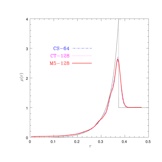
Figure 9: Radial density profiles of the 3D Sedov blast wave test at $t=0.06$. The solid black line indicates the analytic solution, while the simulation profiles are obtained by averaging for each radial bin SPH densities calculated from the particle distributions over a set of grid points located at the surface of a spherical shell and uniformly spaced in angular coordinates. All of the runs were performed using $N=524,288$ particles.

3.4 The blob test

The blob test is another hydrodynamic test where results of standard SPH differ significantly from those produced by grid based simulations (Agertz et al. 2007; Read, Hayfield & Agertz 2010; Cha, Inutsuka & Nayakshin 2010; Heß & Springel 2010; Murante et al. 2011). The test consists of a gas cloud of radius $R_{cl}$ placed in an external medium ten times hotter and less dense than the cloud, so as to satisfy the pressure equilibrium. A large enough wind velocity $v_{W}$ is given to the hot low-density medium so that a strong shock wave strikes the cloud. The interaction of the cloud with the supersonic medium produces a number of effects that are of interest in an astrophysical context, such as gas stripping and fragmentation.

Initially, the blob is perturbed by the development of Richtmyer-Meshkov and Rayleigh-Taylor instabilities (Agertz et al. 2007). After wards, large-scale ($\sim R_{cl}$) KH instabilities are created at the cloud surface because of the shear flows due to the supersonic wind. This non-linear phase is supposed to develop over a time-scale $\tau_{cr}\sim 2R_{cl}\sqrt{\chi}/v_{W}$ (Agertz et al. 2007), where $\chi$ is the density contrast, after which cloud disruption will take place.

In order to investigate the capability of the AC-SPH code to properly follow the hydrodynamic of the blob test, we compare results extracted from a set of SPH simulations realized with the same initial conditions but with different numerical parameters. The numerical setup of the test is the same as in Read, Hayfield & Agertz (2010), to which we refer for more details. A spherical cloud of radius $R_{cl}=197kpc$ is placed in a periodic, rectangular box of size $\{L_{x},L_{y},L_{z}\}=\{2,2,8\}Mpc$. The cloud has density $\rho_{cl}=4.74\times 10^{-33}grcm^{-3}=\chi\rho_{ext}$ and temperature $T_{cl}=10^{6}K=T_{ext}/\chi$. The ambient medium has density and temperature so that $\chi=10$. The cloud is initially located at $\{1,1,1\}Mpc$ and the ambient medium is given a wind velocity $v_{W}=1,000kms^{-1}$, so that for an adiabatic index $\gamma=5/3$ its Mach number is $M=2.7$. An HCP lattice of equal mass particle is constructed in order to satisfy the above density requirements so as to use for this version of the test, a total number of $N\sim 1.1\times 10^{6}$ particles, as in Heß & Springel (2010). Finally, a velocity perturbation is imposed at the cloud surface in order to trigger the development of an instability; amplitude and modes are given in appendix B of Read, Hayfield & Agertz (2010).

We compare results from SPH simulations where three different spline kernels have been used : CS, CRT and $M_{5}$. We use $128$ neighbors for the simulations with the CS and CRT kernels and $220$ for the run with the $M_{5}$ kernel, so that the ratio $\eta$ is the same for all the runs ($\eta\sim 1.5$). For the CS kernel, we run a simulation where the AC term (18) is absent in the equation of thermal energy evolution (CS-128 NOAC), and three other simulations (CS-128, CRT-128, M5-220) in which the AC term (18) is incorporated in the energy evolution equation. In the following, the simulation AV parameters are set as follows: $\{\alpha_{min},\alpha_{max},l_{d}\}=\{0.1,1.5,0.2\}$

For several runs Fig. 10 shows the gas density maps at three different times: $t=1,2,3$; the time being in units of $\tau_{KH}\sim 1.6\tau_{cr}$ (Agertz et al. 2007). The maps have been evaluated according to the SPH prescription on a 2D grid of $(200x800)$ points in the central $yz$ plane located at $x=L_{x}/2$. The top panels of Fig. 10 are for the standard NOAC run CS-128. It can be seen that in this case, unlike what was found in mesh-based simulations (Agertz et al. 2007), the cloud survives the impact of the supersonic wind striking its surface and there is no disruption. This is due to the absence of fluid instabilities developing at the cloud surface. If they were present they would in turn lead to the stripping of material and to the cloud break-up. This code behavior is similar to what was found in previous findings (Agertz et al. 2007; Read, Hayfield & Agertz 2010; Heß & Springel 2010).

On the contrary, incorporating the AC diffusion term in the SPH equations leads to a significant improvement in the code capability to properly model the cloud evolution. This can be seen from the middle and bottom row panels of Fig. 10, in which the density maps are displayed for the CS-128 and M5-220 runs. The simulation performed using the CRT kernel is not shown since its performances are quite similar to those obtained using the CS kernel.

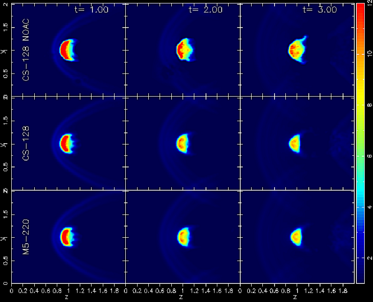
Figure 10: Density maps of the blob test in the central plane $x=L_{x}/2$ at $t=1,2,3$ for SPH runs with (CS, M5) and without (CS NOAC) the AC term. Time is in units of $\tau_{KH}\sim 1.6\tau_{cr}$ and the number accompanying the kernel label indicates the number of neighbors of the run. Axis units are in $Mpc$.

This behavior is consistent with the expectation that introducing AC removes the numerical effects which in SPH prevent the treatment of contact discontinuities when large density jumps are present, and thus the inconsistencies that suppress the growth of the instabilities. The AC-SPH formulation presented here can therefore, at least qualitatively, correctly follow the time evolution of the cloud as in the other SPH schemes which have been recently proposed (Read, Hayfield & Agertz 2010; Heß & Springel 2010; Murante et al. 2011; Saitoh & Makino 2012).

To quantify the code performances in a more quantitative way , Fig. 11 (left panel) shows the mass loss of the cloud as a function of time for the different runs. We follow previous definitions (Agertz et al. 2007) and a gas particle is defined to be still member of the cloud if at the considered epoch its gas and temperature fulfill the conditions $\rho>0.64\rho_{cl}$ and $T<0.9T_{ext}$. The standard SPH results show a cloud that is not disrupted and its mass, after an initial transient, stays constant at about half of the original value. A striking result is instead given by the runs employing the AC term. For these simulations there is now a large mass loss rate occurring at early times, followed by complete cloud disruption at $t\lower 2.15277pt\hbox{$\;\buildrel>\over{\sim}\;$}3\tau_{KH}$.

Note that the mass loss rate of the the AC-SPH runs does not depend in a significant way on the choice of the kernel. This suggests that the cloud disruption is driven by large-scale instabilities and is relatively insensitive to small-scale perturbations. Given the similarities displayed in Fig. 11, left panel, by the mass loss rates of the AC-SPH simulations employing different kernels, when referring to the left panel we will adopt the term mass loss rate to generically indicate the behavior of these curves.

Clearly, in the test considered here the new AC scheme is now capable of properly removing the surface effects, which are present across the contact discontinuity in the standard SPH version, that artificially suppresses the growth of hydrodynamic instabilities. However, a comparison of the mass loss rate with the corresponding one produced using the new moving-mesh code AREPO in simulations of equivalent resolution (Springel 2011, Fig.10), shows that for the AC runs presented here the mass depletion of the cloud occurs much faster. This discrepancy suggests that the processes of heat diffusion which in the adopted numerical scheme are mediated via the AC parameter $\alpha^{C}$, should be somehow constrained by a physically motivated mechanism which has not been previously considered in the discussion of Sect. 2.3. This mechanism should be introduced with the purpose of avoiding a heat transfer mechanism, as governed in the code by Eq. (18), that is overly diffusive.

In order to evaluate the relative effectiveness of heat and momentum transport, in the theory of heat transfer the Prandtl number $Pr$ is defined as the ratio between the kinematic viscosity $\nu$ and the thermal diffusion coefficient $D$: $Pr={\nu}/{D}$ (Blundell & Blundell 2006). For gases, the transport coefficients for the transport of heat and momentum are nearly equal and the Prandtl number is of order unity, with $Pr=\frac{2}{3}$ when $\gamma=5/3$ (Blundell & Blundell 2006). This suggests that a constraint on the particle AC parameter $\alpha^{C}_{i}$ can be obtained by setting

$$Pr\simeq\frac{\nu_{AV}}{D_{AC}}\sim\frac{1}{5}\frac{\alpha^{AV}_{i}v^{AV}_{ij}}{\alpha^{AC}_{i}v^{AC}_{ij}}\lower 2.15277pt\hbox{$\;\buildrel>\over{\sim}\;$}\frac{2}{3}\leavevmode\nobreak\ ,$$ (43)

where the equivalent kinematic viscosity coefficient $\nu_{AV}$ due to AV is given approximately by $\nu^{AV}_{i}\sim\frac{1}{10}{\alpha^{AV}_{i}v^{AV}_{ij}r_{ij}}$ (Lodato & Price 2010), and the numerical heat diffusion coefficient $D^{AC}_{i}$ has been estimated according to Eq. (21). Note that the reverse of Eq. (43) is relatively unimportant, since the source term ${S^{C}}_{i}$ is driven by a second order derivative, whilst for AV is a first order derivative which determines ${S}_{i}$.

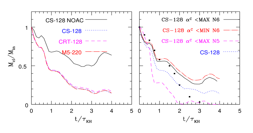
Figure 11: Mass loss of the cloud versus time for the blob test simulations. Particles are defined as cloud member if their temperatures and densities fulfill the conditions $T_{i}<0.9T_{ext}$ and $\rho_{i}>0.64\rho_{cl}$. Left panel: simulations have been performed incorporating the AC term into the SPH equations and using the kernels CS, CRT and $M_{5}$. For the CS kernel a simulation is also shown as reference without AC (NOAC, solid black line). Right panel: for the CS kernel simulations with additional constraints on the particle AC parameters $\alpha^{C}_{i}$ have been performed using $N=10^{6}$ (N6) and $N=10^{5}$ (N5) particles, see text for more details. Black squares have been extracted from Fig. 10 of Springel (2011) and indicate the behavior of the cloud mass versus time in a similar test performed using the moving-mesh code AREPO and with a number of $(64\times 64\times 128)$ resolution elements.

It can be seen that from Eq. (43), for the AC signal velocity adopted here, the constraint on the numerical heat diffusion becomes important in presence of supersonic flows. Moreover, the condition $Pr\sim O(1)$ is valid only for gases, where the transport of momentum and energy occurs simultaneously. For liquids, according to the dominant mechanism of heat conduction, the value of the Prandtl number can vary by several orders of magnitude among different substances (Dimotakis 2005). The condition (43) should, therefore, be considered problem dependent.

A rigorous procedure to derive the upper limits on the set of parameters $\left\{\alpha^{C}_{i}\right\}$ at any given timestep would require to first define for the particle $i$ the numerical kinematic viscosity and heat diffusion coefficients

$$\left\{\begin{array}[]{ l l l }<\nu^{AV}_{i}>&=&|\left(\frac{d\@vec{v}_{i}}{dt}\right)_{AV}|\,\big{/}\,|\nabla^{2}\@vec{v}_{i}+2\@vec{\nabla}\;(\@vec{\nabla}\cdot\@vec{v}_{i})|\\ <D^{AC}_{i}>&=&\left(\frac{du_{i}}{dt}\right)_{AC}\big{/}\nabla^{2}u_{i}\leavevmode\nobreak\ ,\end{array}\right.$$ (44)

where the bulk viscosity $\zeta$ is $5/3$ of the shear viscosity $\eta\equiv\nu\rho$ (Lodato & Price 2010) and it is understood that the SPH expressions should be used for the operators at the denominators.

The upper limits on the parameters $\left\{\alpha^{C}_{i}\right\}$ are then given by the conditions

$$<D^{AC}_{i}>\,\leq\frac{3}{2}<\nu^{AV}_{i}>\leavevmode\nobreak\ ,$$ (45)

which must be simultaneously satisfied by all the parameters. In place of the procedure just described, we adopt here a simpler approach and using Eq. (43) we estimate the upper limits on $\left\{\alpha^{C}_{i}\right\}$ as

$$\alpha^{AC}_{i}\lower 2.15277pt\hbox{$\;\buildrel<\over{\sim}\;$}\frac{3}{10}\alpha^{AV}_{i}MAX_{j<}\left\{|v^{AV}_{ij}|/|v^{AC}_{ij}|\right\}\leavevmode\nobreak\ ,$$ (46)

where the notation $j<$ means that the maximum is taken form all the neighbors $j$ that satisfy the condition $\@vec{v}_{ij}\cdot\@vec{r}_{ij}<0$. This is to be consistent with the definition of AV, for which $\Pi_{ij}$ is non-zero only for approaching particles. Clearly, this definition does not guarantee an accurate estimate of the constraint on the $\alpha^{C}_{i}$ parameter, nonetheless the use of the maximum among all the approaching pairs should provide a floor value for the effective constraint.

For the CS kernel, we then performed a simulation identical to the one previously discussed, but now imposing the additional constraint (46) on the $\alpha^{C}$ parameters. This simulation is labeled as MAX N6 and the corresponding mass loss curve is displayed in the right-hand panel of Fig. 11. In order to assess resolution effects, we ran a mirror simulation now using $N=10^{5}$ particles (MIN N5). Moreover, the uncertainties associated with the use of Eq. (46) can be estimated by looking at the mass loss rate of a simulation (MIN N6) where instead of Eq. (46) the same equation was used but the constraint is derived using the $MIN$ operator instead of the $MAX$ one.

For comparative purposes, in the right-hand panel of Fig. 11 the mass loss of the cloud (black squares), as found in a similar blob test performed by Springel (2011) using the new moving-mesh code AREPO, was also inserted. The number of resolution elements is $64\times 64\times 128$, so that the resolution is approximately equivalent to that of the tests displayed here.

A striking result seen from the behavior of the mass loss rates is that, introducing the constraint (46) on the numerical heat transfer in the simulations, the mass depletion of the cloud is now in better agreement with previous results and in particular with the cloud mass evolution produced in the blob test by the Voronoi-based code AREPO.

Uncertainties associated with the procedure adopted to estimate the constraint on the $\alpha^{C}$ parameters are of limited impact, as can be assessed by the differences between the mass loss rates exhibited by the run MAX N6 and MIN N6. Moreover, for the run MAX N5 the mass loss rate is much stronger than in the case MAX N6. This is indicative of numerical diffusion effects which dominate the blob evolution. Clearly, a numerical simulation with $N=10^{7}$ particles should be required to clarify this issue; however the agreement with previous results of the mass loss for the run MAX N6 suggests that convergence is already being achieved using $N=10^{6}$ particles.

Finally, both the runs MAX N6 and MIN N6 exhibit at $t\lower 2.15277pt\hbox{$\;\buildrel>\over{\sim}\;$}3\tau_{KH}$ a remnant cloud mass which is of the order of $\sim 20-30\%$ of the initial mass. Although such a result can still be due to the use of a constraint on the numerical heat diffusion which still needs to be refined, we note that such remaining masses are equally present in SPH blob tests which have adopted, with the purpose of avoiding the problems of standard SPH, completely different approaches (Heß & Springel 2010; Murante et al. 2011)

We, therefore, suggest that this underestimate in the stripping rate of the blob mass is not due to the AC scheme, but depends rather on the SPH formulation and is associated with the intrinsic errors in gradient estimates. These errors, in turn, lead to the suppression of the small-scale instabilities. Such a issue will be discussed further in detail in Sect. 4.2 dedicated to the Rayleigh-Taylor instability.

To summarize, SPH simulations which incorporate the AC scheme can successfully be used to accurately model the blob evolution. However, the results of the tests indicate that it is necessary to properly constrain the AC parameter $\alpha^{C}$ in order to avoid unphysical heat diffusion when strong supersonic flows are present.

4 Gravity tests

To validate the performances of the AC signal velocity (25), several hydrodynamical test problems were investigated in which the self-gravity must be necessarily taken into account to properly model the system evolution. We first consider the 3D collapse of a cold gas sphere initially at rest, this test being customarily used in SPH to judge the code capability when strong shocks are present, such as those occurring during the formation of self-gravitating structures. We then examine a 2D version of the classic Rayleigh-Taylor instability test and finally the new code is used to assess the behavior of cluster entropies in cosmological structure formation.

4.1 Cold gas sphere

Figure 12: Radially averaged profiles at $t=0.8$ of the Evrard collapse test. Clockwise from the top left panel: profiles of density, entropy, artificial conductivity parameter $\alpha^{C}$ and radial velocity. Curves with different line styles and colors refer to SPH runs performed using different kernels and with (AC) or without (NOAC) the AC term in the SPH energy equation. The black solid lines indicate the 1D PPM reference solution of Steinmetz & Mueller (1993).

A standard hydrodynamical test for SPH codes in which gasdynamics is modeled including self-gravity is the 3D collapse of a cold gas sphere, also commonly recognized as the ’Evrard’ collapse test (Evrard 1988). The test follows in time the adiabatic collapse of a initially cold gas sphere and has been widely used by many authors (Hernquist & Katz 1989; Steinmetz & Mueller 1993; Wadsley, Stadel & Quinn 2004; Springel 2005; Wetzstein et al. 2009; Springel 2010b; Heß & Springel 2010, V11) as a standard test for SPH codes.

The gas cloud is spherically symmetric and initially at rest, with mass $M$, radius $R$, and density profile

$$\rho(r)=\frac{M}{2\pi R^{2}}\frac{1}{r}\leavevmode\nobreak\ .$$ (47)

The gas obeys the ideal gas equation of state with $\gamma=5/3$ and the thermal energy per unit mass is initially set to $u=0.05GM/R$. The SPH simulations are performed using units for which $G=M=R=1$ and the chosen time unit is the cloud free-fall timescale $t_{ff}=(\pi^{2}/8)\sqrt{R^{3}/GM}=\pi^{2}/8$.

With these initial conditions, the pressure support of the gas sphere is negligible and the cloud begins to collapse until a bounce occurs in the core with a subsequent shock wave propagating outward. Most of the kinetic energy is converted into heat at the epoch of maximum compression of the gas, which occurs at $t\sim 1.1$. The initial conditions setup is realized by stretching the radial coordinates of a glass-like uniform distribution of $N=88,000$ equal mass particles located within a sphere of unit radius, so as to generate the density profile of Eq. (47).

To construct the set of SPH simulations, four tests have been run using the kernels CS and $M_{5}$. The number of neighbors is set to $100$ for the $M_{5}$ runs and $50$ for the CS ones. To assess convergence properties in the radial profiles of the considered hydrodynamic variables, the $M_{5}$ run has been replicated using $200,000$ particles ($M_{5}-200k$). All of these runs were performed incorporating in the SPH equations the AC term (18), for the CS kernel a reference run with the AC term disabled has been considered (CS-NOAC). The gravitational softening length is taken as $\varepsilon_{g}=0.02$.

For each test case, we perform simulations with different settings of the AV parameter $l_{d}$. However, introducing a time-dependent AV scheme in SPH reduces numerical viscosity effects and in particular, for the test investigated here, produces a radial entropy profile at the shock front in better agreement with the 1D PPM reference solution. For this reason, the results for different test cases are presented for those runs where a standard AV formulation has been used ( runs $AV_{0}$ of V11). This is done in order to highlight differences in the simulation results due to the use of different kernels and of incorporating the AC term in the SPH thermal energy equation. This choice for the simulation parameters allows one to compare the test calculations performed here with previous results presented in Sect. 5.2 of V11.

The average radial profiles at $t=0.8$ of density, entropy, time-dependent AC parameter and radial velocity are displayed in Fig. 12. The black solid lines indicate the profiles of the 1D PPM calculation of Steinmetz & Mueller (1993). Broadly speaking, one expects to see some differences between the profiles of the NOAC simulation and those of the other runs. This should be valid in particular for the entropy profiles. However, at the considered epoch, Fig. 12 shows that the entropy profile of the NOAC run is still very similar to the others. This occurs because at $t=0.8$ the shock front propagation is still in the early phase and the smoothing in the thermal energy due the AC term is not yet significant.

The behavior of the $\alpha^{C}$ profiles is in accordance with what expected. In particular, the profiles exhibit a peak in correspondence of the shock front location, which occurs approximately at $r\sim 0.18$, and a decay as one moves away from it. There is a dependence on the kernel shape and a weak dependence on resolution. The former is interpreted as a consequence of an improved mixing capability due to the increased order of the kernel. Note that there is a rising in the profiles as one moves toward the sphere center, this occurs because of the presence of a temperature gradient. However, in Eq. (18) this radial dependence is of no effect since behind the shock front the sphere quickly achieves a hydrostatic equilibrium and $v^{AC}_{ij}(grav)\simeq 0$ for $r\lower 2.15277pt\hbox{$\;\buildrel<\over{\sim}\;$}0.1$.

The epoch examined in Fig. 12 has been chosen so as to compare the simulation profiles with the corresponding ones presented in Fig. 40 of Springel (2010b) and realized using the new moving-mesh code AREPO. In particular, a visual inspection shows that ahead of the shock front the accuracy of the entropy profiles shown in Fig. 12 can be considered intermediate between the profile produced using the AREPO code and the one realized with the SPH code Gadget-2 ( right panels in Fig. 40 of Springel (2010b), test cases ‘moving-mesh’ and ‘SPH’, respectively). Note, however, that a strict comparison between the different simulation profiles is difficult because the number of resolution elements employed by Springel (2010b) in the cold gas sphere tests are lower by about $\sim 1/3$ than the one used here. In particular, the smaller shock broadening found here can be ascribed to a resolution effect.

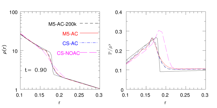
Figure 13: As in Fig. 12, a closer view at $t=0.9$ of the radial profiles of density and entropy in the proximity of the shock front.

Finally, Fig. 13 shows a closer view of the radial density and entropy profiles in the proximity of the shock front at $t=0.9$. The NOAC simulation exhibits now the worst accord with the PPM reference solution, while for the high-resolution run $M_{5}-200k$ the improvement in accuracy is minimal with respect to the other AC runs. This suggests that to obtain a significant improvement in the adherence of the simulation profiles to the PPM solution one must use a much higher number of simulation elements ( say $\lower 2.15277pt\hbox{$\;\buildrel>\over{\sim}\;$}10^{6}$, Springel (2010b) ).

A noteworthy feature of the profiles of Fig. 13 is that now the AC simulation profiles are in much better agreement with the PPM profiles. This is interpreted as a numerical effect in which the pre-shock entropy, which is generated by the AV implementation ahead of the shock front owing to the converging flow, is now strongly reduced because the presence of the AC term in the SPH energy equation now removes this excess of internal energy. This in turn implies, behind the shock front, a thermal energy profile closer to the PPM solution profile.

Comparisons of the profiles of Fig. 13 with the corresponding ones displayed in Fig. 4 of V11 show that the dependency of the simulation profiles on the adopted AC scheme are stronger than the ones due to the time-dependent AV formulation. In fact, these results are almost unaffected if one performs SPH simulations using now a time-dependent AV scheme in place of the standard one.

Finally, two runs have been performed using the CRT and LIQ kernels and a number of neighbors set to $N_{sph}=50$. The profiles of the two simulations have not been shown here to avoid overcrowding in the panels, however the performances of the CRT run are quite similar to those of the CS one, whilst the profiles of the LIQ simulation exhibits very poor consistency properties with respect to the reference PPM solution profiles.

4.2 2D Rayleigh-Taylor

The Rayleigh-Taylor (RT) instability arises when a heavier fluid is placed on the top of a lighter fluid (Chandrasekhar 1961) in presence of an external gravitational field. The fluids are in pressure equilibrium against the external field and in this configuration the system is unstable in the presence of small perturbations at the interface, the lighter fluid will then begin to rise and the denser one to fall. This process leads to the development of characteristic finger-like structures before the fluids enter the non-linear phase where they mix together completely. In order to evaluate the ability of the AC-SPH code to properly describe the evolution of RT instabilities, we consider a 2D version of the test. The initial conditions are chosen to be similar to the numerical test implemented by Abell (2011) to validate its new rpSPH formulation of SPH equations, so as to consistently compare the results. The computational domain consists in a 2D box with coordinates $x\in\{0,1/2\}$, $y\in\{0,1\}$. The boundaries are periodic in $x$ and reflecting in $y$. The density is $\rho_{1}=2$ at the top and $\rho_{2}=1$ at the bottom, with a density profile

$$\rho(y)=\rho_{2}+\frac{(\rho_{1}-\rho_{2})}{\left[1.+\exp{\{-2(y-0.5)/\Delta_{y}\}}\right]}\leavevmode\nobreak\ ,$$ (48)

where $\Delta_{y}=0.05$. This ensures a smoothing in density at the interface $y=0.5$ that allows a consistent numerical behavior (Robertson et al. 2010). This density profile is realized by constructing a HCP lattice of $N=620^{2}$ equal mass particles in which the spacing is varied according to the procedures described in Sect. 3.1.1 until the profile (48) is satisfied.

The pressure at the interface is set to $P_{0}=\rho_{1}/\gamma=10/7$, where $\gamma=1.4$ and it varies with $y$ according to $P(y)=P_{0}-g\rho(y)(y-1/2)$, $g=1/2$ being the external acceleration, so that the system is initially in hydrostatic equilibrium. For the particles that satisfy the condition $|y-0.5|<0.2$ a velocity perturbation is applied in the $y$ direction given by

$$v_{y}(x,y) = \delta v_{y}\{1+\cos[8\pi(x+1/4)]\}$$ (49)

$$\leavevmode\nobreak\ \leavevmode\nobreak\ \leavevmode\nobreak\ \leavevmode\nobreak\ \leavevmode\nobreak\ \{1+\cos[5\pi(y-1/2)]\}/4\leavevmode\nobreak\ ,$$

where $\delta v_{y}=0.1$.

We present results for the CS, CRT, $M_{5}$ and additionally, for reasons which will be discussed later, we consider also the $M_{6}$ kernel (Price 2012, sect. 2.3). The number of neighbors for these runs is set to $N_{sph}=32,32,50,110$, respectively. As in the other test cases considered here, for comparative purposes, we ran a simulation (CS-NOAC) in which the AC term in the thermal energy equation has been disabled. The following settings have been used for the AV parameters: $\{\alpha_{min},\alpha_{max},l_{d}\}=\{0.1,1.5,0.2\}$.

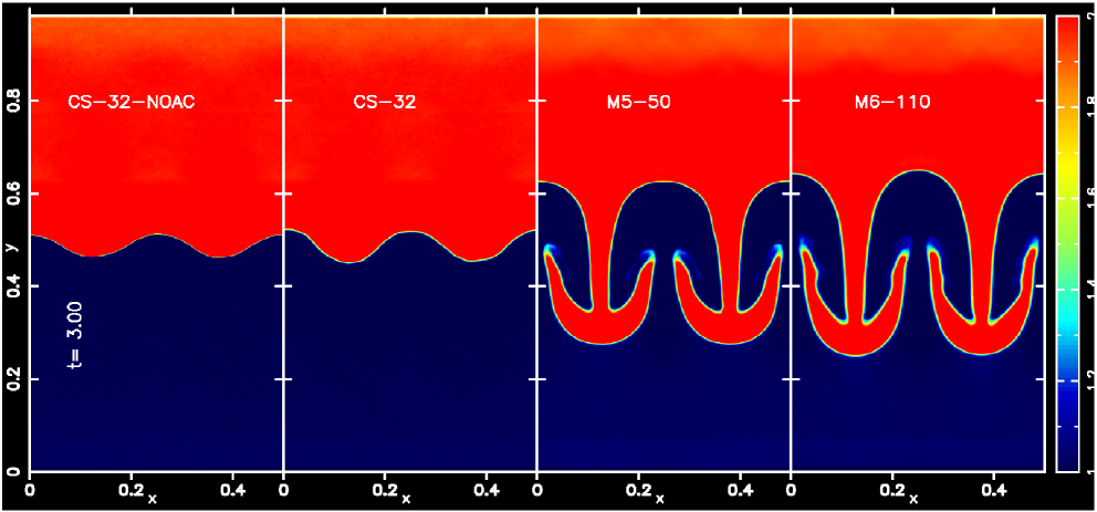
Figure 14: Density maps of the 2D Rayleigh-Taylor tests are shown at time $t=3$ for standard SPH (NOAC) and AC-SPH simulations performed using $N=620^{2}$ particles with different kernels and neighbor numbers. The density distributions can be compared directly with the map shown in Fig. 4 of Abell (2011), top right panel, as the adopted initial conditions for the tests are the same.

In Fig. 14, at the time $t=0.3$, we present the 2D density maps of the different RT tests. As expected, standard SPH is unable to correctly capture the development of the RT instability, as indicated by the leftmost panel of Fig. 14 (CS kernel, NOAC run). However, from this viewpoint the improvement is minimal even for the corresponding AC version of the considered run (CS-32). On the contrary, a significant improvement is obtained if one uses the $M_{5}$ kernel or the next in order $M_{6}$, which is a quintic polynomial (Price 2012). In fact, in the rightmost panel of Fig. 14 ($M_{6}$ run), the center of mass of the RT spikes appears located at a lower position than in the $M_{5}$ run and therefore the convergence might still not be achieved even for the $M_{6}$ run.

This strong dependence of the code performances on the kernel order demonstrates that, for the RT test, accuracy in pressure forces is a fundamental issue. These results are consistent with those of sect. 3.1 and indicate that the poor performances of SPH when handling KH or RT instabilities, in particular for very subsonic flows, are mainly due to the leading errors in the momentum equation. These errors are reduced as the order of the kernel is increased, therefore implying an improved accuracy in pressure force estimates and thus a lower velocity noise. This, in turn, implies a better capability to capture the growth of the instability.

Similar results have recently been obtained by McNally, Lyra & Passy (2011), who ran a suite of 2D KH simulations using carefully crafted initial conditions with the goal of assessing different hydrodynamic code capabilities. The authors conclude that for SPH the code performances are strongly related to the order of the kernel employed in the simulation and thus to the accuracy of the gradient estimates.

Moreover, the simulation behavior of Fig. 14 is consistent with the findings of García-Senz, Cabezón, & Escartín (2012). The authors present a new formulation of SPH in which gradients are estimated using a tensorial approach which conserves both linear and angular momentum. The authors demonstrate that using this higher order gradient estimator the interpolation of physical quantities is significantly improved with respect to the standard method. In particular, several tests showed that the code is now able to successfully capture the development of KH and RT instabilities.

To summarize, the results of this section demonstrate that SPH performances to model hydrodynamic subsonic instabilities depend critically on the accuracy of the gradient estimator. The formulation proposed by García-Senz, Cabezón, & Escartín (2012) looks particularly promising in this aspect to overcome the present SPH difficulties.

Finally, it must be stressed that the simulation results of Fig. 14 have been obtained setting $\delta v_{y}=0.1$. If the same test had been performed using $\delta v_{y}=0.01$, as in the RT test of the new moving-mesh code AREPO (Springel 2010b, Sect. 8.8), the velocity noise would have suppressed the growth of the instability even for the $M_{6}$ run. Note, that in their RT test, García-Senz, Cabezón, & Escartín (2012) were able to recover the growth of the instability using the same amplitude of the velocity perturbation, $\delta v_{y}=0.01$.

4.3 Cluster comparison

In this section, a set of cosmological cluster simulations is constructed using the standard SPH formulation as well as the new AC-SPH version. We only consider non-radiative, or ’adiabatic’ simulations, in which the hydrodynamic is modeled according to the formulation presented in Sect. 2. Previous investigations (Frenk et al. 1999; Wadsley, Stadel & Quinn 2004; Wadsley, Veeravalli & Couchman 2008; Mitchell et al. 2009; Springel 2010b) showed that for the same initial conditions there are systematic differences between results extracted from cluster simulations produced using standard SPH and Eulerian AMR codes. Specifically, the level of central entropy is found to be lower in SPH simulations than in the corresponding AMR runs. The latter simulations are characterized by the presence of a flat entropy core, whereas the radial entropy profile produced by SPH runs increases steadily with radius. As already outlined in the Introduction, the origin of this discrepancy has been the subject of an intense debate (Agertz et al. 2007; Mitchell et al. 2009; Read, Hayfield & Agertz 2010) which has given as main explanation the different degrees of numerical mixing present in the two codes.

To assess the capability of the AC-SPH code in solving this issue, we then run several cluster simulations. A comprehensive study of the differences between the hydrodynamic variables of cluster simulated using the standard and the AC version of the SPH code will be presented in a forthcoming paper. Here, we just show the final radial entropy profile of the simulated clusters as the main variable that can be used to test the effectiveness of the AC-SPH formulation for solving the entropy problem in cluster cores.

A detailed description of the procedures used to construct the simulated cluster sample is given in sect. 2 of V11, we provide a brief summary here. The simulations were carried out assuming a spatially flat ${\Lambda}$CDM model, with matter density parameter $\Omega_{\mathrm{m}}=0.3$, vacuum energy density $\Omega_{\mathrm{\Lambda}}=0.7$, baryonic density $\Omega_{\mathrm{b}}=0.0486$ and $h=H/100kmsec^{-1}Mpc^{-1}=0.7$. The scale-invariant power spectrum is normalized to $\sigma_{\mathrm{8}}=0.9$ on an $8\,h^{-1}$ Mpc scale at the present age $t_{0}$. An N-body cosmological simulation involving only gravity was first run with a comoving box of size $L_{2}=200h^{-1}$Mpc starting from an initial time $t_{in}$ down to the final epoch $t_{0}$. At this epoch clusters of galaxies are identified in the simulation box as groups of particles that are associated with overdensities approximately in excess of $\sim 200\Omega_{\mathrm{m}}^{-0.6}$. Several of these clusters are then resimulated individually using the AC-SPH code here described, coupled with a treecode gravity solver.

Initial conditions for a specified cluster are generated as follows: a spherical region with origin located at the cluster center is populated with a high-resolution (HR) grid, the radius of the HR sphere is such that it contains all of the original particles identified at $t=t_{0}$ as cluster members. A gas and a dark matter particle is associated to each grid node, whose positions are perturbed according to the random realization of the original cosmological simulations and only those particles which are located within the HR sphere are kept for the hydro run. The HR particles are surrounded by a low-resolution shell of dark matter particles, extracted from a grid with spacing twice that of the HR grid, the shell is introduced with the purpose of mimicking the effects of tidal forces. The grid spacing is chosen such that at the end of the procedure a cluster is simulated with $N_{gas}\sim 220,000$ gas particles and $N_{dm}\sim N_{gas}$ dark matter particles in the inner HR sphere, whereas $N^{ext}_{dm}\sim N_{dm}$ are used in the low-resolution shell. Particle masses are assigned according to the values of $\Omega_{\mathrm{m}}$ and $\Omega_{\mathrm{b}}$.

The clusters selected to be re-simulated hydrodynamically were chosen with the following criterion. Originally (V11), the procedure previously described was repeated two more times in order to construct two new cluster samples extracted from cosmological simulations with box sizes $L_{4}=2L_{2}$ and $L_{8}=2L_{4}$. The three cluster samples were then combined to construct a final sample $S_{all}$ of $\sim 160$ clusters covering nearly a decade in cluster masses. Cluster members of sample $S_{all}$ were then ranked according to their dynamical state, as measured by an appropriate statistical indicator. Two sub-samples of four test clusters each, denoted respectively by $Q$ and $P$, were then constructed by extracting from sample $S_{all}$ those clusters with membership criterion for sample $Q$ ($P$) of being in a fully relaxed (perturbed) state. These two sub-samples were then used to investigate the effects of AV in hydrodynamic SPH simulations of galaxy clusters (V11). Here the four test clusters of sub-sample $Q$ were chosen to investigate the performances of the AC-SPH code. This choice being motivated by the need to proper disentangle the amount of entropy mixing produced during merger processes from that specific to the numerical method in the final cluster entropy. The clusters of sub-sample $Q$ were carefully selected on the basis of their dynamical state and are among the most relaxed of sample $S_{all}$. Therefore, for these clusters, differences in the final radial entropy profile between standard and AC runs can be safely ascribed to the new AC term implemented in the code. The AV simulation parameters of the simulations are $\{\alpha_{min},\alpha_{max},l_{d}\}=\{0.1,1.5,0.2\}$.

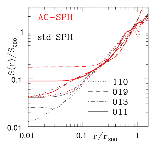
Figure 15: Final radial entropy profiles as a function of $r/r_{200}$ for the four relaxed test clusters. The gas entropy $S(r)=k_{B}T(r)/\mu m_{p}\rho_{g}^{2/3}$ is plotted in units of $S_{200}$ Different line styles refer to different clusters, the numbers indicating the cluster membership in the cosmological ensemble from which they have been extracted. Thin (black) lines are for the profiles of runs performed using the standard SPH formulation, while thick (red) lines refer to the AC-SPH runs incorporating the AC term.

The final entropy profiles for the four test clusters are displayed in Fig. 15, where the cluster entropies have been normalized to

$$S_{200}=\frac{1}{2}\left[\frac{2\pi}{15}\frac{G^{2}M_{200}}{f_{b}H}\right]^{2/3}\leavevmode\nobreak\ ,$$ (50)

where $f_{b}=\Omega_{\mathrm{b}}/\Omega_{\mathrm{m}}$ is the global baryon fraction and $M_{\Delta}=(4\pi/3)\,\Delta\,\rho_{\mathrm{c}}\,r_{\Delta}^{3}$ denotes the mass contained in a sphere of radius $r_{\Delta}$ with mean density $\Delta$ times the critical density $\rho_{\mathrm{c}}=3H^{2}/8\pi G$. As is customary, the cluster mass is defined setting $\Delta=200$ and $r_{200}$ denotes the cluster radius.

The results of Fig. 15 indicate that, although there is a certain degree of scatter between the entropy profiles of individual clusters, nonetheless all of the AC-SPH runs consistently exhibit much shallower entropy profiles and higher core entropies than in the standard SPH runs at $r/r_{200}\lower 2.15277pt\hbox{$\;\buildrel<\over{\sim}\;$}0.1$. For a given cluster, the difference in the levels of central entropies produced by the two codes is about of a factor $\sim 4$, and now the values of central entropies are comparable with those produced using AMR codes in cosmological cluster simulations (Voit, Kay & Bryan 2005) and in idealized cluster binary mergers (Mitchell et al. 2009). It should, however, be stressed that in Eulerian hydrodynamics it is the numerical scheme that forces the fluid to be mixed below the minimum cell size. This suggests that AMR simulations of galxy clusters might overestimate the correct level of core entropy because of fluid mixing (Springel 2010b). To summarize, the development of entropy cores in the AC-SPH runs is clearly a consequence of the heat diffusion term (18), now present in the energy equation. This term acts to redistribute the internal energy produced in the shocks during dissipative processes, so that the subsequent entropy mixing leads, in the end, to higher levels of core entropies.

Similar results were obtained by Wadsley, Veeravalli & Couchman (2008), who similarly added a heat diffusion term to the SPH energy equation, but using the prescription (26) instead of the Eq. (18) adopted here. According to Wadsley, Veeravalli & Couchman (2008), the value of the coefficient $C$ tends to be problem dependent and for the cluster simulations the best agreement with the entropy profiles extracted from the mesh code runs is obtained setting $C\simeq 0.1-1$. Here, the time-dependent formulation (22) presents the advantage of minimizing thermal diffusion away from shocks, as demonstrated in the cold gas sphere test by Fig. 12, where the radial profile of the AC parameter $\alpha^{AC}$ is peaked at the shock location.

The simulations presented in this section have been realized using adiabatic gas physics. However, a realistic modeling of the intra-cluster medium physics must incorporate the possibility that the gas cools radiatively. Previous simulations (V11) showed that the presence of cooling leads to the development in the inner cluster regions of dense compact cool gas cores and subsequently of high levels of turbulence, the latter being produced by the hydrodynamical instabilities generated by the interaction of the compact cool cores with the ambient medium.

How this scenario is affected by incorporating into the SPH equations a numerical heat diffusion term is an issue which can be properly addressed only by resorting to numerical simulations. Here, we outline that two competing effects are expected to influence the final level of turbulence in a cluster core: the improved capability of the code to describe the development of hydrodynamical instabilities, and thus an increase in the amount of turbulence, and the reduced availability of cool gas because of the presence of material of higher entropy which has been brought in the inner core due to the enhanced fluid-mixing properties of the code.

Finally, a resolution study was already performed in V11, indicating for the simulation resolution employed here a substantial stability in the entropy profiles of the simulations. Although the simulations of V11 do not incorporate the AC term, we do not expect strong variations in the resolution dependence of the profiles, given the similarity of the level of core entropies with those found using mesh-based codes.

5 Summary and conclusions

In this paper, we have presented an SPH numerical scheme which incorporates an artificial conductivity term and uses an appropriate signal velocity for simulations including gravity. The AC formulation has been introduced by Price (2008) as a solution to the problems encountered by standard SPH to correctly follow the development of KH instabilities, due to the inconsistencies of the standard formulation in the description of density at contact discontinuity. Here, a suite of hydrodynamic test problems is investigated with the purpose of validating the new AC-SPH code and to assess its performances when using the specifically adopted signal velocity.

The results of the KH instability test are presented in Sect. 3.1, in which the code capabilities have been tested by considering SPH simulations of the KH test performed using a large variety of initial condition set-up and SPH kernels. The set of initial conditions has been chosen as in Valcke et al. (2010), so as to consistently compare the results. These are in accordance with the corresponding ones of Valcke et al. (2010) and indicate that, for the version of the KH test analyzed here, the AC implementation is important for the long-term behavior of the simulation.

Moreover, the results of the KH test indicate (Valcke et al. 2010; Read, Hayfield & Agertz 2010; McNally, Lyra & Passy 2011) that the poor performances of standard SPH to properly treat KH instabilities can be explained in terms of two distinct effects. The first is a general problem of consistency, which for the problem under consideration requires that smooth interfaces should be present at contact discontinuities, in order to obtain numerical convergence. The second effect which in standard SPH suppresses the growth of KH instabilities is the leading error in the momentum equation, due to incomplete kernel sampling (Read, Hayfield & Agertz 2010) and quantified by the norm $\@vec{E}^{0}$ defined by Eq. (36).

To circumvent this problem several proposals have been made (Valcke et al. 2010; Read, Hayfield & Agertz 2010) in which the standard SPH cubic spline $M_{4}$ kernel is replaced by the new LIQ or CRT kernels with steeper central profiles. These kernels present the advantage of being stable against particle clumping, so that the number of neighbors can be safely increased in order to reduce the error $\@vec{E}^{0}$.

In this paper, we consider the possibility of reducing sampling errors by considering higher-order $B-$spline kernels, specifically the $M_{5}$ or quartic spline kernel. A striking result of the KH runs presented in sect. 3.1 is that, for a given value of the ratio $\eta$ between the smoothing length and the mean interparticle spacing, simulations of the KH test performed using the $M_{5}$ kernel have amplitudes of the $\@vec{E}^{0}$ error substantially smaller and in line with the behavior of the same quantity for simulations employing the LIQ or CRT kernels. A linear stability analysis reveals that this result follows owing to the very good stability properties of the $M_{5}$ kernel, in fact the analysis suggests that the clumping instability is absent for values of $\eta$ up to $\eta\lower 2.15277pt\hbox{$\;\buildrel<\over{\sim}\;$}2$, which in 3D corresponds to $N_{sph}\sim 520$ neighbors.

These findings are consistent with the recent results of Dehnen & Aly (2012) who proposed to adopt, with the specific purpose of avoiding the clumping instability, the Wedland (1995) functions as a new class of kernels. The authors showed that in terms of stability and accuracy properties, the quartic spline performs extremely well when compared with the proposed Wedland functions. These results are strictly connected to the properties of the kernel Fourier transform, which according to the authors must be non-negative to avoid particle clumping, and are consistent with the findings of sect. 3.1.3 since increasing the kernel order both the $B-$spline and the Wedland functions approach the Gaussian.

We therefore propose, as a compromise between the need of reducing sampling errors while keeping the computational cost at a minimum, the use of the $M_{5}$ kernel with neighbor number in the range $N_{sph}\sim 60-120$ as the standard combination which guarantees sufficient accuracy in many SPH simulations of astrophysical problems. Moreover, the results of the Sod shock tube test of sect. 3.2 demonstrate that in order to obtain simulation profiles in accordance with the analytic solution, for simulations employing kernels with a modified shape the use of a much larger number of neighbors than in the case of the $M_{5}$ runs is necessary.

The results of the gravity tests show that the adoption of the AC-SPH scheme significantly reduces, at the level tested in this paper, the differences seen in the hydrodynamics between standard SPH and grid-based simulations of self-gravitating structures. For the cold gas sphere, the entropy profile is in better agreement with the PPM reference solution and for the cosmological cluster simulations, a key result is the final level of core entropies, which are consistent with those of the central entropies produced using AMR codes. Thus, it appears that in hydrodynamic simulations where self-gravity is important the AC term, accompanied by the proposed signal velocity, plays a key role as a mechanism of redistributing thermal energy and hence as a source of entropy mixing.

To summarize, results extracted from simulations of hydrodynamic tests where self-gravity dominates are in much better agreement with the corresponding ones obtained using mesh-based codes. The results then demonstrate the capability of the implemented AC-SPH scheme to properly follow the formation of cosmic structures.

It is worth noting that the artificial heat conduction term was originally proposed by Price (2008) with the purpose of avoiding the inconsistencies encountered by standard SPH in presence of density steps at contact discontinuities. A complementary view has been proposed by Wadsley, Veeravalli & Couchman (2008), who introduced the same term, albeit in a different numerical formulation, with the aim of modeling the level of diffusion due to turbulence. The two interpretations are not mutually inconsistent, however the results of the self-gravity tests presented in this paper support the view of a heat diffusion term which in SPH is capable of mimicking the diffusion due to turbulence. In a similar fashion, Violeau & Issa (2007) presented an SPH scheme to model a free-surface incompressible flow which , in analogy with 3D Large Eddy Simulations, assumes a Smagorinsky (1963) model for the filtered Navier-Stokes equations.

The results of the blob test simulations demonstrate that the instabilities leading to the expected cloud disruption can develop only when the SPH energy equation incorporates the AC term. A particularly interesting result is that an appropriate limiting condition must be implemented on the AC coefficients $\alpha^{C}$ in order to avoid an unphysical amount of heat diffusion, which in turn leads to a cloud disruption which occurs too early. This limiter has been identified as given by the Prandtl number and, for the AC signal velocity adopted here, it severely limits the amplitude of the AC coefficients in the regime of strong supersonic flows.

AC-SPH simulations of the blob test incorporating now the new constraint support this view, since Fig. 11 shows for the new runs a cloud mass-loss rate which is in better agreement with the rates obtained from simulations realized using a completely independent numerical scheme (Springel 2011). However, it must be stressed that the condition (43) has been calculated for a perfect monoatomic gas with $\gamma=5/3$, so that a physically motivated constraint on the artificial heat diffusion of the simulated medium should be considered problem dependent.

However, the code has still several problems which render its use problematic if the development of hydrodynamic instabilities need to be followed in the regime of subsonic flows. The results of the simulations indicate that these shortcomings are not due to the AC implementation, but rather are intrinsic in the standard formulation with which gradients are calculated in SPH and the related errors are subsequently introduced in the momentum equation. In particular, simulations of the RT test show that increasing the kernel order alleviates the problems but does not solve them. These results are in accordance with recent findings (McNally, Lyra & Passy 2011; García-Senz, Cabezón, & Escartín 2012) and clearly demonstrate that for very subsonic flows, the poor performances of SPH to model hydrodynamic instabilities are strictly connected to the code accuracy in gradient estimates.

The formulation of García-Senz, Cabezón, & Escartín (2012), which has been proposed with the aim of calculating SPH gradients with an as high as possible accuracy while keeping the benefits of a Lagrangian formulation, looks in this aspect very promising and suggests further investigations along the numerical approach proposed in this paper. These would be particularly relevant in the light of the recent results of Bauer & Springel (2012), who claim that standard SPH fails to properly model the regime of subsonic turbulence. They reach their conclusions by comparing results extracted from simulations of driven subsonic turbulence realized using the moving-mesh code AREPO and GADGET SPH. Their results have been criticized by Price (2012), for whom the use of a time-dependent AV is critical in SPH simulations of subsonic turbulence.

A re-analysis of the Bauer & Springel (2012) simulations using the AC-SPH code presented here, augmented with improved gradient operators, would then be of fundamental importance to achieve a deeper understanding of the capability of different numerical methods to model subsonic turbulence. The latter being expected to have a significant impact in shaping the thermodynamic properties of baryons in cosmological haloes and, subsequently, the process of galaxy formation.

References

- Abell (2011) Abel, T., 2011, MNRAS, 413, 271
- Agertz et al. (2007) Agertz, O., Moore, B., Stadel, J., Potter, D., Miniati, F., Read, J., Mayer, L., Gawryszczak, A., Kravtsov, A., Nordlund, Å, Pearce, F., Quilis, V., Rudd, D., Springel, V., Stone, J., Tasker, E., Teyssier, R., Wadsley, J. & Walder, R., 2007, MNRAS, 380, 963
- Balsara (1995) Balsara, D., 1995, J. Comp. Phys., 121, 357
- Bauer & Springel (2012) Bauer, A. & Springel, V., 2012, MNRAS, 423, 2558
- Berger & Colella (1989) Berger, M. J. & Colella, P., 1989, J. Comp. Phys., 82, 64
- Blundell & Blundell (2006) Blundell, S. J. & Blundell, K. M., 2006, Concepts in Thermal Physics, Oxford University Press
- Børve, Omang & Trulsen (2004) Børve, S., Omang, M. & Trulsen, J., 2004, ApJS, 153, 447
- Brookshaw (1985) Brookshaw, L., 1985, Proc. of the Astrn. Society of Australia, 6, 207
- Cha, Inutsuka & Nayakshin (2010) Cha, S.-H., Inutsuka, S.-I. & Nayakshin, S., 2010, MNRAS, 403, 1165
- Chandrasekhar (1961) Chandrasekhar, S., 1961, Hydrodynamic and hydromagnetic stability, Oxford University Press
- Colella & Woodward (1984) Colella, P. & Woodward, P. R., 1984, J. Comp. Phys., 54, 174
- Cullen & Dehnen (2011) Cullen, L. & Dehnen, W., 2011, MNRAS, 408, 669
- Dehnen & Aly (2012) Dehnen, W. & Aly, H., 2012, arXiv:1204.2471
- Dimotakis (2005) Dimotakis, P. E., 2005, Ann. Rev. Fluid Mech., 37, 329
- Dolag et al. (2005) Dolag, K., Vazza, F., Brunetti, G. & Tormen, G., 2005, MNRAS, 364, 753
- Evrard (1988) Evrard, A. E., 1998, MNRAS, 235, 911
- Frenk et al. (1999) Frenk, C. S., White, S. D. M., Bode, P., Bond, J. R., Bryan, G. L., Cen, R., Couchman, H. M. P., Evrard, A. E., Gnedin, N., Jenkins, A., Khokhlov, A. M., Klypin, A., Navarro, J. F., Norman, M. L., Ostriker, J. P., Owen, J. M., Pearce, F. R., Pen, U.-L., Steinmetz, M., Thomas, P. A., Villumsen, J. V., Wadsley, J. W., Warren, M. S., Xu, G. & Yepes, G., 1999 , ApJ, 525, 554
- Fryxell et al. (2000) Fryxell, B., Olson, K., Ricker, P., Timmes, F. X., Zingale, M., Lamb, D. Q., MacNeice, P., Rosner, R., Truran, J. W. & Tufo, H., 2000 ApJS, 131, 273
- Fulk & Quinn (1996) Fulk, D. A. & Quinn, D. W., 1996, J. Comp. Phys., 126, 165
- García-Senz, Cabezón, & Escartín (2012) García-Senz, D., Cabezón, R. M., Escartín, J. A., 2012, A&A, 538, A9
- Gingold & Monaghan (1977) Gingold, R. A. & Monaghan, J. J., 1977, MNRAS, 181, 375
- Hernquist & Katz (1989) Hernquist, L. & Katz, N., 1989 ApJS, 70, 419
- Heß & Springel (2010) Heß, S. & Springel, V., 2010 , MNRAS, 406, 2289
- Hubber et al. (2011) Hubber, D. A., Batty, C. P., McLeod, A. & Whitworth, A. P., 2011, A&A, 529, A27
- Inutsuka (2002) Inutsuka, S.-I., 2002, J. Comp. Physics, 179, 238
- Junk et al. (2010) Junk, V., Walch, S., Heitsch, F., Burkert, A., Wetzstein, M., Schartmann, M. & Price, D., 2010, MNRAS, 407, 1933
- Kravtsov, Klypin & Khokhlov (1997) Kravtsov, A. V., Klypin, A. A. & Khokhlov, A. M., 1997, ApJS, 111, 73
- Lodato & Price (2010) Lodato, G. & Price, D. J., 2010, MNRAS, 405, 1212
- Lucy (1977) Lucy, L. B., 1977 , Astr. Journal, 82, 1013
- McNally, Lyra & Passy (2011) McNally, C. P., Lyra, W. & Passy, J.-C., 2011, arXiv:1111.1764
- Merlin et al. (2010) Merlin, E., Buonomo, U., Grassi, T., Piovan, L. & Chiosi, C., 2010, A&A, 513, A36
- Mitchell et al. (2009) Mitchell, N. L., McCarthy, I. G., Bower, R. G., Theuns, T. & Crain, R. A., 2009 , MNRAS, 395, 180
- Monaghan (1997) Monaghan, J. J., 1997, J. Comp. Physics, 136, 298
- Morris & Monaghan (1997) Morris, J. P. & Monaghan, J. J., 1997, J. Comp. Physics, 136, 41
- Monaghan (2000) Monaghan, J. J., 2000, J. Comp. Physics, 159, 290
- Monaghan (2005) Monaghan, J. J., 2005, Reports on Progress in Physics, 68, 1703
- Morris (1996) Morris, J. P., 1996, Analysis of Smoothed Particle Hydrodynamics with Applications, Ph.D. Thesis, Monash University , Melbourne
- Murante et al. (2011) Murante, G., Borgani, S., Brunino, R. & Cha, S.-H., 2011, MNRAS, 417, 136
- Norman & Bryan (1999b) Norman, M. L. & Bryan, G. L., 1999b, in Numerical Astrophysics, Astrophysics and Space Science Library Vol. 240, ed. S. M. Miyama, K. Tomisaka, & T. Hanawa (Kluwer, Boston) , 19
- Norman (2005) Norman, M. L., 2005, The Impact of AMR in Numerical Astrophysics and Cosmology, in Adaptive Mesh Refinement – Theory and Applications. Springer, Berlin, New York, vol. 41 of Plewa T., Linde T., Weirs V.G, eds, Lecture Notes in Computational Science and Engineering, p. 413.
- O’Shea et al. (2005a) O’Shea, B. W., Bryan, G., Bordner, J., Norman, M. L., Abel, T., Harkness, R. & Kritsuk, A., 2005a, Introducing Enzo, an AMR Cosmology Application, in Adaptive Mesh Refinement – Theory and Applications, ed. T. Plewa, T. Linde, V.G. Weirs (Berlin; New York: Springer), vol. 41 of Lecture Notes in Computational Science and Engineering, p. 341.
- Price (2005a) Price, D. J., 2005, Ph. D. thesis, astro-ph/0507472
- Price & Monaghan (2005) Price, D. J. & Monaghan, J. J., 2005, MNRAS, 364, 384
- Price (2008) Price, D.J., 2008, J. Comp. Phys. , 227, 10040
- Price (2012) Price, D. J., 2012, J. Comp. Phys., 231, 759
- Price (2012b) Price, D. J., 2012b, MNRAS, 402, L33
- Rasio & Lombardi (1999) Rasio, F. A. & Lombardi, J. C. jr., 1999, J. Comp. Phys., 109, 213