Fluctuation induced luminescence sidebands in the emission spectra of resonantly driven quantum dots

Abstract

We describe how complex fluctuations of the local environment of an optically active quantum dot can leave rich fingerprints in its emission spectrum. A new feature, termed “Fluctuation Induced Luminescence” (FIL), is observed to arise from extremely rare fluctuation events that have a dramatic impact on the response of the system—so called “black swan” events. A quantum dissipative master equation formalism is developed to describe this effect phenomenologically. Experiments performed on single quantum dots subject to electrical noise show excellent agreement with our theory, producing the characteristic FIL sidebands.

Walter Schottky Institut and Physikdepartment, Technische Universität München, Am Coulombwall 4, 85748 Garching, Germany]Walter Schottky Institut (München) [Física Teórica de la Materia Condensada, Universidad Autónoma de Madrid, 28049, Madrid, Spain]Universidad Autónoma de Madrid Walter Schottky Institut and Physikdepartment, Technische Universität München, Am Coulombwall 4, 85748 Garching, Germany]Walter Schottky Institut (München) Physikdepartment, Technische Universität München, James Franck Str., 85748 Garching, Germany]Technische Universität München Walter Schottky Institut and Physikdepartment, Technische Universität München, Am Coulombwall 4, 85748 Garching, Germany]Walter Schottky Institut (München) QD,QDM,PL

Discrete solid-state quantum emitters such as III-V quantum dots¹ and NV-centers² represent highly versatile hardware for all-optical quantum technologies. In particular, self-assembled InGaAs Quantum Dots (QDs) are robust, ultra narrow linewidth sources of triggered single photons and polarization-entangled photon pairs.³ The creation of remote entanglement via photon-interference³ calls for discrete emitters that produce Fourier-transform limited single photon wave packets. This is very difficult to achieve in solid-state systems since the system typically undergoes frequency jitter due to fluctuations of the charge environment of the system^{4, 5, 6} and unavoidable coupling to the lattice.^{7, 8} However, for low temperatures and weak optical driving, coupling to the lattice is inhibited⁹ and the spectral lineshape is expected to reflect slow fluctuations of the environment which manifest themselves as discrete spectral jumps and wandering¹⁰. Fourier transform-limited lines are typically not achieved in optical experiments, with measured linewidths somewhat above the theoretical limit^{11, 12, 13, 14}. While spectral fluctuations in self-assembled QDs have been investigated with non-resonant excitation^{15, 16}, the impact of a fluctuating environment in the case of true resonant excitation has received significantly less attention. Spectral fluctuations arising from environmental fluctuations are a common feature in condensed matter systems arising also for colour centers in diamond¹⁷, colloidal nanocrystals¹⁸ and semiconductor nanowire quantum dots¹⁹.

Here, we probe the impact of environmental fluctuations on the optical response of a resonantly driven quantum emitter embedded within an electrically tunable solid-state environment.^{20, 21} The resonant excitation simplifies the picture since it avoids complications due to incoherently injected carriers, such as fluctuations arising from charge (de)trapping at defects in the wetting later. It also allows to consider only a single projection of spin by using circularly polarized excitation. As depicted schematically in 1(a), we consider a situation where a narrowband single frequency laser coherently excites the interband p-transition in a single dot and the emission from the s-shell is monitored.²² The corresponding Hamiltonian reads:

$$H=(\Delta-E_{21})\left|1\right\rangle\left\langle 1\right|+\Delta\left|2\right\rangle\left\langle 2\right|+\Omega(\left|0\right\rangle\left\langle 2\right|+\left|2\right\rangle\left\langle 0\right|)$$ (1)

where $\Delta=\omega_{2}-\omega_{\mathrm{L}}$ is the detuning between the state 2 (interband p-transition) and the laser, and $E_{21}=\omega_{2}-\omega_{1}$ the energy gap between the p and s-interband transitions (we set $\hbar=1$ for convenience). The relaxation between the p and s-shells—due to, e.g., phonon mediated processes²³—occurs at the rate $\gamma_{21}$ and is included as an incoherent relaxation in the Lindblad form, $\frac{\gamma_{21}}{2}\mathcal{L}_{\left|1\right\rangle\left\langle 2\right|}$ where, for any operator $c$, $\mathcal{L}_{c}$ is the Liouville superoperator defined as $\mathcal{L}_{c}(\rho)=2c\rho c^{{\dagger}}-c^{{\dagger}}c\rho-c^{{\dagger}}c\rho$. The radiative decay of the s-state giving rise to luminescence is also described as $\frac{\gamma_{10}}{2}\mathcal{L}_{\sigma}$ where $\sigma=\left|0\right\rangle\left\langle 1\right|$. The photoluminescence (PL) spectrum $S(\omega,\Delta)$ is obtained by calculating $G^{(1)}(\tau)=\langle\sigma^{{\dagger}}(0)\sigma(\tau)\rangle$ from the master equation $\partial_{t}\rho=i[\rho,H]+\frac{\gamma_{21}}{2}\mathcal{L}_{\left|1\right\rangle\left\langle 2\right|}(\rho)+\frac{\gamma_{10}}{2}\mathcal{L}_{\sigma}(\rho)$ and taking the Fourier transform. Setting as the reference energy, the energy at which the s-state emits when $\Delta=0$ (with maximum gain), the result reads:

$$S(\omega,\Delta)=\frac{1}{\pi}\frac{\frac{8\gamma_{21}\Omega^{2}}{\gamma_{10}(\gamma_{21}^{2}+4\Delta^{2})+4\Omega^{2}(2\gamma_{10}+\gamma_{21})}\Big{(}\gamma_{10}(\Gamma^{2}+4\omega^{2})+4\Omega^{2}\Gamma\Big{)}}{(\gamma_{10}^{2}+4(\omega-\Delta)^{2})(\Gamma^{2}+4\omega^{2})+8\Omega^{2}(\gamma_{10}\Gamma-4(\omega-\Delta)\omega)+16\Omega^{4}}$$ (2)

where we introduced $\Gamma\equiv\gamma_{10}+\gamma_{21}$.

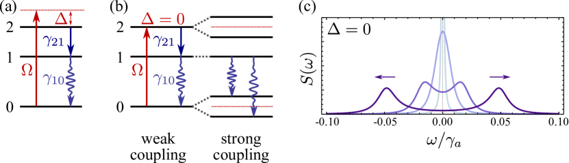
Figure 1: (a) The level structure under study, (b) dressing of the p-state at resonance and (c) the Mollow doublet which arises from it. The laser is tuned closed to the excited p orbital, labelled 2. Incoherent relaxation $\gamma_{21}$ transfers the excitation to the s-state, labelled 1, which PL is detected. When the excitation rate $\Omega$ is large enough, the laser dresses the states which are driven, namely, the p-state and the ground state. The latter, being common with the s-state, result in the observation of a Mollow doublet with splitting increasing linearly with $\Omega$.

This is the full quantum picture which describes saturation of the two-level system and dressing of the p-state by the laser when the pumping $\Omega$ is large.²⁴ In this case, this results in a spectral doublet rather than the Mollow triplet for a two-level system,²⁵ because relaxation is from the naked s-state to the dressed ground state, which is common to both the bare s and driven p levels, as shown in 1(b). Provided that the gain is large enough, this configuration might have advantages as compared to resonance fluorescence, since excitation and detection are detuned and pump photons can be filtered from the emission.

In the linear regime, Eq. (2) assumes the much simpler form:

$$S(\omega,\Delta)=\frac{2\Omega^{2}\pi}{\gamma_{10}}\times\frac{1}{\pi}\frac{\gamma_{21}/2}{(\gamma_{21}/2)^{2}+\Delta^{2}}\times\frac{1}{\pi}\frac{\gamma_{10}/2}{(\gamma_{10}/2)^{2}+(\omega-\Delta)^{2}}+O(\Omega)^{4}\,,$$ (3)

with $O(\Omega^{4})$ terms of at least fourth order in $\Omega$. This shows that the coherently excited QD luminescence is given simply by the product of $i)$ the emitted intensity, $ii)$ the population gain of the driven detuned oscillator, and $iii)$ the Lorentzian PL lineshape of emission; an extremely simple and fundamental result. The emitted intensity grows linearly with $\Omega^{2}$ as long as the system remains in the linear regime under its effective pumping $P_{\mathrm{eff}}$, that is, as long as $\mathrm{Gain}(\Delta)=P_{\mathrm{eff}}/\gamma_{10}\ll 1$. At resonance $\Delta=0$, where the driving is most efficient, the condition reads $\mathrm{Gain}(0)=4\Omega^{2}/(\gamma_{21}\gamma_{10})\ll 1$. We will restrict our discussion to the linear regime in the remainder of the manuscript, where one expects only emission from the s-shell directly to the ground state by direct radiative recombination. Plotting the intensity of emission of the s-state photons (in colour, with lighter shades corresponding to higher intensities) detected at a given energy (on the $x$ axis) for the various detunings of the lasers with the p-state (on the $y$ axis), this produces a tilted line, since the emission linearly tracks the energy detuning from resonance. This feature is presented by the diagonally shifting transition shown in 2(a). The horizontal line superimposed at $\Delta=0$ arises from the strong enhancement of the emission signal at resonance, termed “gain” in the discussion below.

Measurements were made on many different single quantum dots and QD-Molecules (QDMs)^{26, 27} to test the predictions of this theory. As discussed below and presented in 2(b), the experimental findings differ significantly from these simple expectations. The samples investigated were GaAs n-i–Schottky photodiodes containing a low density layer of InGaAs self-assembled QDs or vertically stacked QDMs. Such structures facilitate control of the static electric field in the vicinity of the nanostructure via an applied voltage. The growth conditions used gave rise to QD nanostructures with a large radius (30-50nm) and, thus, a large oscillator strength as evidenced by measurements of short radiative lifetimes for self-assembled nanostructures ($\leq 700$ps, limited by the temporal resolution of our setup). Individual QDs or QDMs were excited optically using a tunable single frequency laser and their photoluminescence was recorded using a low temperature confocal microscope. Photoluminescence excitation (PLE) spectra from the same dot were obtained by recording the emission in the vicinity of s-shell transition with a CCD camera while scanning the laser energy through the excited orbital states of the system—fully analogous to the theoretical scheme introduced in the discussion related to 1. A typical experimental result is presented in 2(b) in a false colour representation for excitation in the range 9-13meV above the s-shell neutral exciton transition. An unexpected vertical line is clearly observed, labelled FIL in 2(b), that is pinned to zero detuning. The energy gap between this newly observed FIL feature and the s-shell emission is identical to the detuning of the laser from the p-shell transition. In a configuration where the single mode laser was fixed and the p and s transition were shifted, for instance by application of an electric field to tune the levels through the DC Stark effect, we obtained identical results. This observation was also found to hold for QD-molecules pumping the antibonding branch of the neutral, coupled exciton²⁸ and detecting the bonding branch. Here, the energy gap between the two transitions involved varies with electric field²⁷ but the FIL peak always appears at the energy of maximum gain. We will now show that this striking phenomenology is fully accounted for by fluctuations, albeit of a particular type.

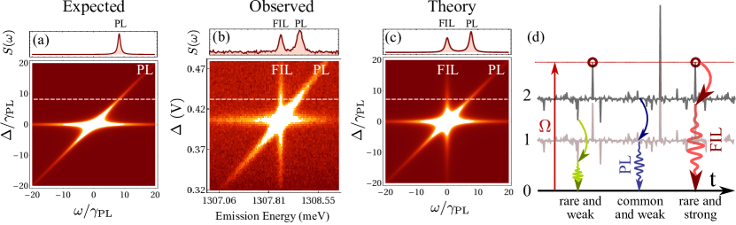
Figure 2: (a) The expected luminescence from a resonantly driven QD in the linear regime: the diagonal transition shows the radiative recombination of the s shell as the frequency of the driving field is detuned from the excited state, while the horizontal line reflects the high increase of the excitation efficiency of the driven oscillator. (b) A new peak—FIL—appears in the experimental observation as a vertical line pinned by the laser. (c) The theory supplemented with fluctuations reproduces the observed phenomenology. (d) Scheme of the processes which give rise to FIL. The levels 1 and 2 have scalefree fluctuations which, when they bring the system into resonance, result in a strong absorption and subsequent emission.

We proceed with the introduction of fluctuations in the theoretical model, an undertaking that is nontrivial at a microscopic level²⁹. Our modelling remains rooted in the master equation approach and hinges on a reservoir that can be in any of $N_{R}+1$ configurational states, labelled as $R=-N_{R}/2,\ldots,0,\ldots,N_{R}/2$, each of which has the effect of shifting the levels of our system according to $\omega_{iR}=\omega_{i}+R\delta$, $i=1,2$. Such a picture has been introduced by Budini³⁰ with a small reservoir to describe blinking. Here, we will assume that the reservoir is large enough to approximate a continuous fluctuating bath, introducing the need of a continuous distribution for the fluctuations. The driven QD Hamiltonian now depends on the states of the reservoir:

$$\tilde{H}_{R}=(\Delta-E_{21}+R\delta)\left|1R\right\rangle\left\langle 1R\right|+(\Delta+R\delta)\left|2R\right\rangle\left\langle 2R\right|+\Omega(\left|0R\right\rangle\left\langle 2R\right|+\left|2R\right\rangle\left\langle 0R\right|)$$ (4)

where we use a ‘~’ symbol to denote that a fluctuating environment has been included in the picture. The states $\left|iR\right\rangle$, with $i=0,1$ or 2, correspond to the case where the QD is in the state $\left|i\right\rangle$ and the reservoir in its configuration $R$. Note that the latter is not a proper quantum number, but a label to index a macrostate for the environment. We assume that only the energy of the levels fluctuates while other parameters remain unchanged. In this case, the master equation of the system now reads:

$$\partial_{t}\rho_{R}= i[\rho_{R},\tilde{H}_{R}]+\frac{\gamma_{10}}{2}\mathcal{L}_{\left|0R\right\rangle\left\langle 1R\right|}(\rho_{R})+\frac{\gamma_{21}}{2}\mathcal{L}_{\left|1R\right\rangle\left\langle 2R\right|}(\rho_{R})$$ (5a)

$$- \sum_{R^{\prime}}\phi_{R\rightarrow R^{\prime}}\rho_{R}+\sum_{R^{\prime}}\phi_{R^{\prime}\rightarrow R}\rho_{R^{\prime}}\,.$$ (5b)

We assume that the transitions between the configurational states of the reservoir do not depend on the state of the system. As neither the initial condition nor the dynamics introduces any coherence between the bath macrostates, their density matrix can be written as $\rho_{Env}=\sum_{R}\mathcal{P}_{R}\left|R\right\rangle\left\langle R\right|$ where $\mathcal{P}_{R}=\mathrm{Tr}_{S}(\rho_{R})$ are the populations. The fluctuations between the configurational states of the reservoir are, therefore, ruled by a classical evolution: $\partial_{t}\mathcal{P}_{R}=-\sum_{R^{\prime}}\phi_{R\rightarrow R^{\prime}}\mathcal{P}_{R}+\sum_{R^{\prime}}\phi_{R^{\prime}\rightarrow R}\mathcal{P}_{R^{\prime}}$, defining the kinetic dynamics of the environment. On the other hand, the system dynamics arise after tracing out all internal transitions between the configurational states of the reservoir, $\rho=\sum_{R}\rho_{R}$. Therefore, the evolution of the system density matrix is non-Markovian, $\partial_{t}\rho=\mathbf{L}(\rho)+\int_{0}^{t}d\tau\mathcal{K}(t-\tau)\rho(\tau)$, where $\mathbf{L}$ represents the unitary dynamics in the absence of the reservoir and $\mathcal{K}$ the memory kernel introduced by it. One can compute the kernel analytically when the number of $R$-states is small. In this case, the steady state ($t=0$) correlator is $G^{(1)}(\tau)=\sum_{R,R^{\prime}}\langle\sigma^{\dagger}_{R^{\prime}}(0)\sigma_{R}(\tau)\rangle$ where $\sigma_{R}=\left|0R\right\rangle\left\langle 1R\right|$. Introducing an auxiliary matrix $\theta_{R}$ that follows the same master equation as the conditional density matrix $\rho_{R}$ but with initial conditions (i. c.) that depend on a different state of the reservoir $R^{\prime}$, i.e., $\langle k|\theta_{r}(0)|l\rangle=\delta_{r,R^{\prime}}\delta_{l,0}\langle k|\rho_{R^{\prime}}|1\rangle$, each correlator $\langle\sigma^{\dagger}_{R^{\prime}}(0)\sigma_{R}(\tau)\rangle$ can be computed in terms of the elements of $\theta_{R}$ according to $\langle\sigma^{\dagger}_{R^{\prime}}(0)\sigma_{R}(\tau)\rangle=\sum_{k,l}\langle k|\theta_{R}(\tau)|l\rangle\langle l|\sigma_{R}|k\rangle=\langle 1|\theta_{R}(\tau)|0\rangle$. With this, the total correlator reads:

$$G^{(1)}(\tau)=\sum_{R}\Big{\{}\sum_{R^{\prime}}\Big{[}\langle 1|\theta_{R}(\tau)|0\rangle\Big{]}_{\text{i.~{}c.: }\langle k|\theta_{R^{\prime}}(0)|0\rangle=\langle k|\rho_{R^{\prime}}|1\rangle}\Big{\}}\,.$$ (6)

Its Fourier transform provides the PL spectrum $\tilde{S}(\omega,\Delta)$ in the fluctuating environment. The formalism is general and can be applied to arbitrary quantum optical systems where fluctuations are believed to play an important role^{31, 32}.

Now that we have formally included the fluctuations at a microscopic level, we need to specify their character. They have been left completely arbitrary in the discussion until now. Since Gauss introduced his law of errors³³, the so-called “normal distribution” became the archetypal fluctuation in physical systems. Its importance and universality stems from the central limit theorem, that states that the normal distribution arises from averaging a sufficiently large number of random variables, regardless of which distribution rules their fluctuations on an individual basis (provided some properties to which we return shortly). While the normal (ergodic) type of fluctuations describes much of the physical word, it can fail dramatically for highly complex systems. A different class of fluctuations, for which the central limit theorem does not hold, provides a new paradigm. They are known as power law or fat-tail type of distributions,³⁴ the most famous and widespread type of which is, in physics, the Lorentzian. The main property of such fluctuations is that they are scalefree, that is, the fluctuator can wander arbitrarily far from its most likely position, in contrast with a normal distribution where $5\sigma$ deviations are so unlikely that they are regarded as “discovery” of a new physics (the concept of “standard deviation” is rooted in the normal distribution and has no counterpart for scalefree fluctuators). When it is combined with impact of the outliers, scalefree fluctuations give rise to new notions such as kurtosis-risk, extreme-risk³⁵ and “black swans”³⁶—highly unlikely events that can totally alter the trajectory or response of the system.

In the following, we assume that our elementary quantum optical system is embedded in such an environment that has scalefree fluctuations. We will assume a Lorentzian type of fluctuation, but qualitatively similar results would follow from other types of scalefree fluctuations. We are thus left to express the rates $\phi_{R\rightarrow R^{\prime}}$ which enforce the steady state solution of $\partial_{t}\mathcal{P}_{R}=-\sum_{R^{\prime}}\phi_{R\rightarrow R^{\prime}}\mathcal{P}_{R}+\sum_{R^{\prime}}\phi_{R^{\prime}\rightarrow R}\mathcal{P}_{R^{\prime}}$ to be proportional to the Lorentzian distribution $\mathcal{P}_{R}=\frac{1}{\mathcal{N}}\frac{1}{\pi}\frac{\gamma_{F}/2}{(\gamma_{F}/2)^{2}+(R\delta)^{2}}$, with $\sum_{R}\mathcal{P}_{R}=1$. $\mathcal{N}$ is the normalization constant that removes the units (and can be simplified in the continuum limit) $\mathcal{N}=\sum_{R}\frac{1}{\pi}\frac{\gamma_{F}/2}{(\gamma_{F}/2)^{2}+(R\delta)^{2}}\approx\frac{1}{\delta}\int dx\frac{1}{\pi}\frac{\gamma_{F}/2}{(\gamma_{F}/2)^{2}+x^{2}}=\frac{1}{\delta}$. This is obtained with rates of the form:

$$\phi_{R\rightarrow R^{\prime}}=\phi\mathcal{P}_{R^{\prime}}\approx\frac{\phi}{\delta}\frac{1}{\pi}\frac{\gamma_{F}/2}{(\gamma_{F}/2)^{2}+(R^{\prime}\delta)^{2}}\,,$$ (7)

with $\phi$ the speed of fluctuations. They only depend on the final state. The transition towards the central point has the largest rate, being the most likely one no matter from which point the transition is initiated.

We can now solve these equations numerically. A typical result is presented in 2(c) and, clearly, reproduces the same phenomenology observed in our experiments; namely the unexpected emission line, denoted “FIL” for Fluctuation Induced Luminescence. This new line arises from the fluctuations as sketched in 2(d): when the system is far detuned, it infrequently wanders into resonance with the laser by the very nature of the scalefree fluctuation that allows such giant deviations. The photo-generated electron-hole pair will then relax into the s-shell before emitting light. Depending on the speed of the fluctuations, the emitted photon can either have the frequency of the most likely s-shell energy when the fluctuations are faster than the recombination time, or it can have a frequency which is detuned from the most likely s-shell energy when the fluctuations are slower than the recombination time. The strong absorption gain which occurs there compensates for the combined scarcity and brevity of these events. This is depicted in 2(d) with Lorentzian fluctuations of the levels as a function of time with three highlighted emission processes: i) from an extreme outlier which emits far from the most likely s-state energy, producing no notable luminescence as such events are rare and emit weakly, ii) from a state close to the most likely s-state energy, producing PL as a result of the many times this weak-emission configuration is realized, and iii) from an extreme outlier which, by chance, brings the system into resonance, producing detectable luminescence from the strong emission compensating for the rarity of such events. Our system, therefore, implements “black-swans” in the solid state: extremely rare occurrences that have a huge impact and result in a qualitative change in the system.

One can study from numerical solutions the properties of the FIL peak. Depending on parameters (such as when $\gamma_{21}<\gamma_{F}$ and $\phi$ is small), the FIL peak is sharper and brighter than the PL. Interestingly, it is found that the speed of fluctuations is an important ingredient that determines the form of the detuning dependent FIL and PL emission. Faster fluctuations decrease the intensity of FIL leaving its linewidth essentially unchanged. In the limit of slow fluctuations, numerical solutions converge towards the analytical expression obtained by integrating the photoluminescence spectrum over its fluctuations: $\tilde{S}(\omega,\Delta)=\int_{-\infty}^{\infty}S(\omega,\delta)\frac{1}{\pi}\frac{(\gamma_{F}/2)}{(\gamma_{F}/2)^{2}+(\delta-\Delta)^{2}}\,d\delta$. Plugging Eq. (3) in this expression, one can compute the slow Lorentzian fluctuations PL spectrum in the linear regime in a closed form: it is the sum of two peaks, with their Lorentzian and dispersive parts given by:

$$S(\omega,\Delta)=\frac{\Omega^{2}/\gamma_{10}}{\Big{[}(\frac{\gamma_{F}-\gamma_{21}}{2})^{2}+\Delta^{2}\Big{]}\Big{[}(\frac{\gamma_{F}+\gamma_{21}}{2})^{2}+\Delta^{2}\Big{]}}\sum_{p=\mathrm{FIL\,,PL}}\frac{1}{\pi}\Big{[}\frac{L_{p}\gamma_{p}/2-K_{p}(\omega-\omega_{p})}{(\gamma_{p}/2)^{2}+(\omega-\omega_{p})^{2}}\Big{]}\,,$$ (8a)

$$\omega_{\mathrm{FIL}}=0\,,\quad\gamma_{\mathrm{FIL}}=\gamma_{10}+\gamma_{21}\,,\quad L_{\mathrm{FIL}}=\gamma_{F}\Big{[}\frac{\gamma_{F}^{2}-\gamma_{21}^{2}}{4}+\Delta^{2}\Big{]}\,,\quad K_{\mathrm{FIL}}=-\gamma_{F}\gamma_{21}\Delta\,,$$ (8b)

$$\omega_{\mathrm{PL}}=\Delta\,,\quad\gamma_{\mathrm{PL}}=\gamma_{10}+\gamma_{F}\,,\quad L_{\mathrm{PL}}=\gamma_{21}\Big{[}\frac{\gamma_{21}^{2}-\gamma_{F}^{2}}{4}+\Delta^{2}\Big{]}\,,\quad K_{\mathrm{PL}}=\gamma_{F}\gamma_{21}\Delta\,.$$ (8c)

This fully describes the properties of the peaks depending on the system parameters and the amplitude of fluctuations when they are slow. This shows in particular that the peak which is sharper is also the one that is the more intense. Not all these attributes are conserved in the exact numerical solution when the speed of fluctuations is not very slow, but at least the qualitative result is spelt out and easily understood in this limiting case.

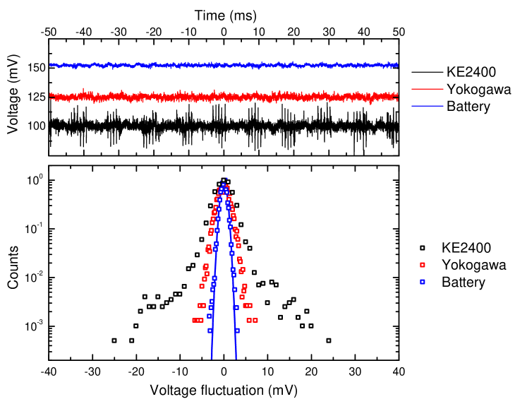
Figure 3: Fluctuations due to the voltage source. The upper row shows a trace of the applied voltage over a 10ms window, for three sources: (a) a standard Keithley KE2400 source, (b) a Yukogawa source and (c) a simple battery. Beside larger amplitudes of fluctuations the Keithley and Yukogawa have fluctuations to all orders, that is, infrequent but large deviation from the applied voltage. These are the cause of FIL.

The FIL peak in the experiment is observed when the excitation laser is detuned by $\Delta\leq 0.5$meV from the excited orbital state resonance. At the largest detunings where FIL is still clearly observable, defined as being when its intensity is at least 1/4 of that of the PL, the system would be more than 20 standard deviations away from the median if it would follow a normal distribution. The probability for the system to fluctuate into resonance according to the Lorentzian distribution is approximately one in a million. However, since the quantum dynamics occurs over picosecond timescales, and the spectra are recorded with integration times extending over several minutes, this still leaves sufficient opportunities for these extremely rare events to occur and give rise to the FIL peak in the spectrum. They are observable as compared to off-resonant cases thanks to their huge impact. The same probability is completely negligible according to the Gaussian distribution and would not be once realized, even if running the experiment over several lifetimes of the universe.

Fingerprints of non-ergodic fluctuations are actually commonplace in the emission from individual solid state emitters, including flurophores such as molecules,³⁷ proteins and polymers,^{38, 39} semiconductor quantum dots,^{40, 10} nanorods⁴¹ and nanowires. Ubiquitous phenomenology such as fluorescence intermittency^{42, 40} and spectral wandering⁴³ are observed arising from coupling to their local environment. In our system, the source of the fluctuation was traced to be fluctuations of the programmable voltage source in which electronics stabilize the output voltage. Scalefree fluctuations are of an entirely counterintuitive character and the cause of many unpredictable and important events in complex environments, such as catastrophes on financial markets⁴⁴ or sudden large-scale changes in meteorological systems.³⁵ In our case, tracing their origin to the electronics in the setup was a difficult and time-consuming task since such fluctuations are typically invisible to the spectral noise of the devices. Furthermore, such unlikely events do not appear in the technical description of the source provided by the manufacturer. It is not established, for instance, that they are exactly of the Lorentzian type, but their fat-tail property is mandatory to understand our experimental observations. In most experiments, such extremely rare fluctuations of voltage have no impact whatsoever. It requires the black-swan character, only met in particular configurations such as ours, stemming from the extremely large gain of the QD absorption driven quasi resonantly that make these rare events impactful. In our QDs and QDMs, their effect was remarkable since they produced a new line in the emission spectrum. The FIL shown in 2 was obtained with a Keithley 2400 voltage source. We have repeated the experiment using a Yokogawa voltage source, and observed that the FIL peak reduced significantly in intensity, although it did not disappear completely. We have been able to remove the scalefree fluctuations entirely by using a simple battery-driven voltage follower circuit. The voltage traces measured for these three sources are shown in 3. The KE2400 series clearly exhibits random fluctuations with large deviations from the median, resulting in a clear characteristic fat-tail profile in its distribution (see the lower panel in 3). The Yokogawa source, on the other hand, appears much more Gaussian-like with no observable large departures. The fact that a FIL is still observed shows that it, too, features extreme outliers with scalefree properties, but that we are unable to record them in the time windows over which the voltage was monitored. The difficulty to detect and characterize power-law distributions is a well-known problem of statistical analysis.⁴⁵ By turning these elusive outliers into black swans, our system therefore implements a way to probe and characterize such fluctuations. It could allow, for instance, to quantify the range over which the power law holds, one of the most difficult practical problem in the field. Such fluctuations could also be intrinsic, for instance from trapping of a carrier in a nearby defect, with fluctuations in the induced electric field correlated with the time spent by the carrier in the trap, which being memoryless in time would result in Lorentzian fluctuations. In our case, however, we can rule out such possibilities from a temperature series for the conventional and fluctuation-induced luminescence, both shown in 4. While the conventional PL exhibits the characteristic phonon-sidebands with their hallmark asymmetry at low temperature,⁷ the FIL is temperature independent, showing that it has no connection with the intrinsic fluctuation spectrum or dynamic of the system.

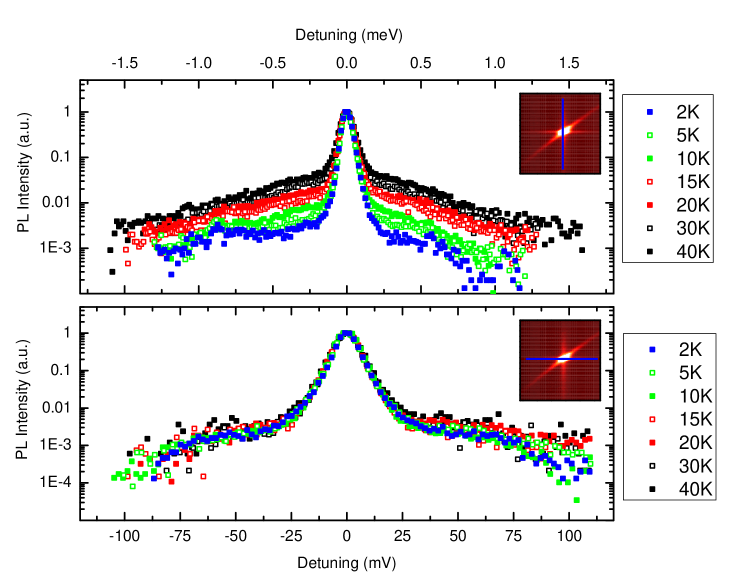
Figure 4: Temperature series for the cross-section of (a) luminescence at resonance and (c) FIL. While the former exhibits a clear and characteristic temperature dependence, the FIL is temperature independent, pointing at an extrinsic origin for the scalefree fluctuations causing it.

In conclusion, we have presented a general theory of fluctuations in a dissipative quantum optical system and applied it to the case of a resonantly driven quantum dot in the presence of scalefree fluctuators. We have shown that in a system exhibiting strong gain, the combination of rare and impactful events may result in drastic and qualitative changes in the system, known in the stochastic literature as “black swan events”. In our case, a new sharp line pinned at the laser excitation is produced. This type of luminescence has never been reported before to the best of our knowledge, and further investigations are needed to study whether they might prove useful for applications and/or characterization. The system we have presented could be used as a sensitive probe of its fluctuating environment and a powerful gauge of power-law tails. Although such fluctuations could be intrinsic to the system, we have reported here an experimental occurrence that was put forward, most unexpectedly, by the voltage source apparatus, and an enduring puzzle was put to rest with a simple battery.

This work is funded by the Deutsche Forschungsgemeinschaft via Grant No. SFB-631 and the excellence cluster Nanosystems Initiative Munich and the European Union via SOLID (FP7-248629) and S3Nano (FP7-289795). FPL acknowledges support from the Marie Curie IEF “SQOD”, EdV from the Alexander von Humboldt Foundation. G.A. also thanks the Technische Universität München Institute for Advanced Study for support.

References

- Wang 2008 Self-Assembled Quantum Dots; Wang, Z. M., Ed.; Springer, 2008
- Awschalom et al. 2007 Awschalom, D. D.; Epstein, R.; Hanson, R. Sci. Am. 2007, 297, 84
- Salter et al. 2010 Salter, C. L.; Stevenson, R. M.; Farrer, I.; Nicoll, C. A.; Ritchie, D. A.; Shields, A. J. Nature 2010, 465, 594
- Fry et al. 2000 Fry, P. W. et al. Phys. Rev. Lett. 2000, 84, 733
- Vamivakas et al. 2011 Vamivakas, A. N.; Zhao, Y.; Fält, S.; Badolato, A.; Taylor, J. M.; Atatüre, M. Phys. Rev. Lett. 2011, 107, 166802
- Houel et al. 2012 Houel, J.; Kuhlmann, A. V.; Greuter, L.; Xue1, F.; Poggio, M.; Gerardot, B. D.; Dalgarno, P. A.; Badolato, A.; Petroff, P. M.; Ludwig, A.; Reuter, D.; Wieck, A. D.; Warburton, R. J. Phys. Rev. Lett. 2012, 108, 107401
- Muljarov et al. 2005 Muljarov, E. A.; Takagahara, T.; Zimmermann, R. Phys. Rev. Lett. 2005, 95, 177405
- Ramsay et al. 2010 Ramsay, A. J.; Gopal, A. V.; Gauger, E. M.; Nazir, A.; Lovett, B. W.; Fox, A. M.; Skolnick, M. S. Phys. Rev. Lett. 2010, 104, 017402
- Langbein et al. 2004 Langbein, W.; Borri, P.; Woggon, U.; Stavarache, V.; Reuter, D.; Wieck, A. D. Phys. Rev. B 2004, 70, 033301
- Robinson and Goldberg 2000 Robinson, H. D.; Goldberg, B. B. Phys. Rev. B 2000, 61, 5086(R)
- Högele et al. 2004 Högele, A.; Seidl, S.; Kroner, M.; Karrai, K.; Warburton, R. J.; Gerardot, B. D.; Petroff, P. M. Phys. Rev. Lett. 2004, 93, 217401
- Atatüre et al. 2006 Atatüre, M.; Dreiser, J.; Högele, A. B. A.; Karrai, K.; Ĭmamoḡlu, A. Science 2006, 28, 551
- Xu et al. 07 Xu, X.; Sun, B.; Berman, P. R.; Steel, D. G.; Bracker, A. S.; Gammon, D.; Sham, L. J. Science 07, 317, 929
- Vamivakas et al. 2009 Vamivakas, A. N.; Zhao, Y.; Lu, C.-Y.; Atatüre, M. Nat. Phys. 2009, 5, 198
- Berthelot et al. 2006 Berthelot, A.; Favero, I.; Cassabois, G.; Voisin, C.; Delalande, C.; Roussignol, P.; Ferreira, R.; Gérard, J. M. Nat. Phys. 2006, 2, 759
- Latta et al. 2009 Latta, C.; Högele, A.; Zhao, Y.; Vamivakas, A. N.; Maletinsky, P.; Kroner, M.; Dreiser, J.; Carusotto, I.; Badolato, A.; Schuh, D.; Wegscheider, W.; Atature, M.; Ĭmamoḡlu, A. Nat. Phys. 2009, 5, 758
- Robledo et al. 2010 Robledo, L.; Bernien, H.; van Weperen, I.; Hanson, R. Phys. Rev. Lett. 2010, 105, 177403
- Müller et al. 2004 Müller, J.; Lupton, J. M.; Rogach, A. L.; Feldmann, J.; Talapin, D. V.; Weller, H. Phys. Rev. Lett. 2004, 93, 167402
- Sallen et al. 2010 Sallen, G.; Tribu, A.; Aichele, T.; André, R.; Besombes, L.; Bougerol, C.; Richard, M.; Tatarenko, S.; Kheng, K.; Poizat, J.-P. Nat. Photon. 2010, 4, 696
- Flagg et al. 2009 Flagg, E. B.; Muller, A.; Robertson, J. W.; Founta, S.; Deppe, D. G.; Xiao, M.; Ma, W.; Salamo, G. J.; Shih, C. K. Nat. Phys. 2009, 5, 203
- Muller et al. 2007 Muller, A.; Flagg, E. B.; Bianucci, P.; Wang, X. Y.; Deppe, D. G.; Ma, W.; Zhang, J.; Salamo, G. J.; Xiao, M.; Shih, C. K. Phys. Rev. Lett. 2007, 99, 187402
- Ester et al. 2007 Ester, P.; Lackmann, L.; de Vasconcellos, S. M.; Hübner, M. C.; Zrenner, A.; Bichler, M. Appl. Phys. Lett. 2007, 91, 111110
- Heitz et al. 2001 Heitz, R.; Born, H.; Guffarth, F.; Stier, O.; Schliwa, A.; Hoffmann, A.; Bimberg, D. Phys. Rev. B 2001, 64, 241305(R)
- Cohen-Tannoudji and Reynaud 1977 Cohen-Tannoudji, C. N.; Reynaud, S. J. phys. B.: At. Mol. Phys. 1977, 10, 345
- Mollow 1969 Mollow, B. R. Phys. Rev. 1969, 188, 1969
- Müller et al. 2011 Müller, K.; Reithmaier, G.; Clark, E. C.; Jovanov, V.; Bichler, M.; Krenner, H. J.; Betz, M.; Abstreiter, G.; Finley, J. J. Phys. Rev. B 2011, 84, 081302(R)
- Müller et al. 2012 Müller, K.; Bechtold, A.; Ruppert, C.; Zecherle, M.; Reithmaier, G.; Bichler, M.; Krenner, H. J.; Abstreiter, G.; Holleitner, A. W.; Villas-Boas, J. M.; Betz, M.; Finley1, J. J. Phys. Rev. Lett. 2012, 108, 197402
- Krenner et al. 2005 Krenner, H. J.; Sabathil, M.; Clark, E. C.; Kress, A.; Schuh, D.; Bichler, M.; Abstreiter, G.; Finley, J. J. Phys. Rev. Lett. 2005, 94, 057402
- Richter et al. 2009 Richter, M.; Carmele, A.; Sitek, A.; Knorr, A. Phys. Rev. Lett. 2009, 103, 087407
- Budini 2009 Budini, A. A. Phys. Rev. A 2009, 79, 043804
- Hennessy et al. 2007 Hennessy, K.; Badolato, A.; Winger, M.; Gerace, D.; Atature, M.; Gulde, S.; Fălt, S.; Hu, E. L.; Ĭmamoḡlu, A. Nature 2007, 445, 896
- Ota et al. 2009 Ota, Y.; Kumagai, N.; Ohkouchi, S.; Shirane, M.; Nomura, M.; Ishida, S.; Iwamoto, S.; Yorozu, S.; Arakawa, Y. Appl. Phys. Express 2009, 2, 122301
- Gauss 1809 Gauss, C. F. Theoria motus corporum coelestium in sectionibus conicis solem ambientium; Reprint by Cambridge Library Collection (2011), 1809
- Coles 2001 Coles, S. An Introduction to Statistical Modeling of Extreme Values; Springer, 2001; ISBN 978-1-85233-459-8
- Garrett and Müller 2008 Garrett, C.; Müller, P. Bull. Amer. Meteor. Soc. 2008, 89, 1733
- Taleb 2007 Taleb, N. N. The Black Swan; Random House, 2007
- Hoogenboom et al. 2005 Hoogenboom, J. P.; van Dijk, E. M. H. P.; Hernando, J.; van Hulst, N. F.; Garcá-Parajó, M. F. Phys. Rev. Lett. 2005, 95, 097401
- Dickson et al. 1997 Dickson, R. M.; Cubitt, A. B.; Tsien, R. Y.; Moerner, W. E. Nature 1997, 388, 355
- Bout et al. 1997 Bout, D. A. V.; Yip, W.-T.; Hu, D.; Fu, D.-K.; Swager, T. M.; Barbara, P. F. Science 1997, 277, 1074
- Nirmal et al. 1996 Nirmal, M.; Dabbousi, B. O.; Bawendi, M. G.; Macklin, J. J.; Trautman, J. K.; Harris, T. D.; Brus, L. E. Nature 1996, 383, 802
- Wang et al. 2006 Wang, S.; Querner, C.; Emmons, T.; Drndic, M.; Crouch, C. H. J. Phys. Chem. B 2006, 110, 23221
- Frantsuzov et al. 2008 Frantsuzov, P.; Kuno, M.; Jankó, B.; Marcus, R. A. Nat. Phys. 2008, 4, 519
- Empedocles et al. 1996 Empedocles, S. A.; Norris, D. J.; Bawendi, M. G. Phys. Rev. Lett. 1996, 77, 3873
- Mandelbrot and Hudson 2004 Mandelbrot, B.; Hudson, R. L. The (Mis)behavior of Markets; Basic Books, 2004
- Clauset et al. 2009 Clauset, A.; Shalizi, C. R.; Newman, M. E. J. SIAM Rev. 2009, 51, 661