Finite-sample equivalence in statistical models for presence-only data
Abstract
Statistical modeling of presence-only data has attracted much recent attention in the ecological literature, leading to a proliferation of methods, including the inhomogeneous Poisson process (IPP) model, maximum entropy (Maxent) modeling of species distributions and logistic regression models. Several recent articles have shown the close relationships between these methods. We explain why the IPP intensity function is a more natural object of inference in presence-only studies than occurrence probability (which is only defined with reference to quadrat size), and why presence-only data only allows estimation of relative, and not absolute intensity of species occurrence.
All three of the above techniques amount to parametric density estimation under the same exponential family model (in the case of the IPP, the fitted density is multiplied by the number of presence records to obtain a fitted intensity). We show that IPP and Maxent give the exact same estimate for this density, but logistic regression in general yields a different estimate in finite samples. When the model is misspecified—as it practically always is—logistic regression and the IPP may have substantially different asymptotic limits with large data sets. We propose “infinitely weighted logistic regression,” which is exactly equivalent to the IPP in finite samples. Consequently, many already-implemented methods extending logistic regression can also extend the Maxent and IPP models in directly analogous ways using this technique.
doi:
10.1214/13-AOAS667keywords:
and
tWillSupported by NSF VIGRE Grant DMS-0502385. tTrevSupported in part by NSF Grant DMS-10-07719 and NIH Grant RO1-EB001988-15.
1 Introduction.
In recent years ecologists have devoted significant attention to the problem of estimating the geographic distribution of a species of interest from records of where it has been found in the past. There are many motivations for solving this problem, including planning wildlife management actions, monitoring endangered or invasive species, and understanding species’ response to different habitats. A great variety of experimental designs and statistical methods exist for tackling this problem, and can be found in the literature on resource-selection functions [Manly et al. (2002), Lele and Keim (2006)], case-augmented designs [Lee, Scott and Wild (2006), Dorazio (2012)] and site occupancy modeling [MacKenzie (2006)].
Ecologists have proposed many statistical methods for modeling such data, including the inhomogeneous Poisson process (IPP) model [Warton and Shepherd (2010)], maximum entropy (Maxent) modeling of species distributions [Phillips, Dudík and Schapire (2004), Phillips, Anderson and Schapire (2006), Phillips and Dudík (2008)] and the logistic regression model along with its various generalizations such as GAM, MARS and boosted regression trees [Hastie, Tibshirani and Friedman (2009)]. See Elith et al. (2006) for discussion and comparison of these and other methods in common use.
In recent years several articles have emerged detailing connections between the three modeling methods above. Each method takes as its input a presence-only data set along with a set of background points consisting of a regular grid or random sample of locations in some geographic region of interest. Warton and Shepherd (2010) showed that logistic regression estimates converge to the IPP estimate when the size of the presence-only data set is fixed and the background sample grows infinitely large. Aarts, Fieberg and Matthiopoulos (2012) additionally described a variety of models for presence-only and other data sets whose likelihoods may all be derived from the IPP likelihood. Renner and Warton (2013) further explore the connection between Maxent and the IPP, taking up the important issue of how we might check the IPPs modeling assumptions.
Our primary aim in writing this paper is to provide additional clarity to this topic, recapitulating and deriving the results in a unified framework and extending them in several directions. We view all three major methods as solutions to the same parametric density estimation problem.
1.1 Presence-only data.
Modeling of species distributions is simplest and most convincing when the observations of species presence are collected systematically. In a typical design, a surveyor visits a one-square-kilometer patch of land for one hour and records how many specimens she discovers in that interval. The records of unsuccessful surveys are called absence records, a mild misnomer since ecologists recognize that specimens could be present but go undetected. A data set reflecting presence or absence of a species in each sampling unit is called presence–absence data.
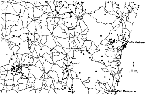
Unfortunately, dedicated surveys recording sampling effort are expensive, especially for rare or elusive species. For many species of interest, the only data available are museum or herbarium records of locations where a specimen was found and reported, for instance, by a motorist or hiker. Typically these presence-only records are collected haphazardly and frequently suffer from unknown sampling bias such as that illustrated in Figure 1. The clustering of koala sightings near roads and cities probably has more to do with the behavior of people than of koalas.
In recent years many such presence-only data sets have become available electronically, and geographic information systems (GIS) enable ecologists to remotely measure a variety of geographic covariates without having to visit the actual locations of the observations. As a result, presence-only data has become a popular object of study in ecology [Elith et al. (2006)].
1.2 What should we estimate?
Before we can sensibly decide how to model presence-only data, we must address the issue of what it is we are modeling in the first place. How should we think of “species occurrence,” the scientific phenomenon nominally under study? This issue arises with presence-only and presence–absence data alike.
1.2.1 Occurrence probability.
Figure 2 is a typical “heat-map” output of a study of the willow tit in Switzerland using count data [Royle, Nichols and Kéry (2005)]. The map reveals which locations are more or less favored by the species (in this case, high elevation and moderate forest cover appear to be the bird’s habitat of choice). The legend tells us that the color of a region reflects the local probability of “occurrence.”
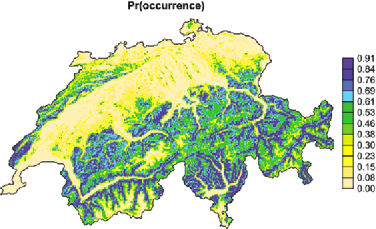
But precisely what event has this probability? Reading the paper, we discover that occurrence means that there is at least one willow tit present on a survey path through a 1 km1 km quadrat of land. In this case, the authors analyze a presence–absence data set using a hierarchical model that explicitly accounts for the possibility that a bird was present but not detected at the time of the survey.
Because the survey path length varies across sampling units, the authors use it in their model as a predictor of presence probability. It is not specified which value of this predictor is used in generating the heat map, which makes the map difficult to interpret.
Even if we could interpret the heat map as the probability of a bird being present anywhere in the quadrat (not just along a path of unspecified length), this probability would still be larger in a 2 km2 km sampling unit and smaller in a 100 m100 m one. Therefore, the very definition of “occurrence probability” in a presence–absence study depends crucially on the specific sampling scheme used to collect the presence–absence data. Consequently, interpreting the legend of such a heat map can only make sense in the context of a specific quadrat size, namely, whatever size was used in the study. We would recommend that this information always be displayed alongside the plot to avoid conveying the false impression (suggested by a heat map) that occurrence probability is an intrinsic property of the land, when it is really an extrinsic property.
Though the choice of quadrat size used to define occurrence probability is ecologically arbitrary, it can in principle yield estimates with meaningful interpretations. By contrast, estimating occurrence probability in a presence-only study is a murkier proposition. Any method purporting to do so without reference to quadrat size would be predicting the same occurrence probability within a large or small quadrat, which cannot make sense.
1.2.2 Occurrence rate.
Since occurrence probability is only meaningful with reference to a specific quadrat size, it is a somewhat awkward quantity to model in a presence-only study. In this context it is more natural to estimate an occurrence rate or intensity: that is, a quantity with units of inverse area (e.g., 1km2) corresponding to the expected number of specimens per unit area. Under some simple stochastic models for species occurrence, including the Poisson process model considered here, specifying the occurrence rate is equivalent to specifying occurrence probability simultaneously for all quadrat sizes.
Unfortunately, a presence-only data set only affords us direct knowledge of the expected number of specimen sightings per unit area. The absolute sightings rate is reflected in the number of records in our data set, but, at best, this rate is only proportional to the occurrence rate discussed above, which typically is the real estimand of interest. We must assume that our sightings only constitute a small fraction of the species’ population over our study region, possibly with repeated sightings of the same specimen. Without other data or assumptions we would have no way of knowing what this constant of proportionality might be.
In other words, the absolute sightings rate is observable but usually not of direct interest, while the absolute occurrence rate is interesting but not observable without another source of information. Using presence-only data alone, we can at best hope to estimate a relative, not absolute, occurrence rate. Even assuming that the sightings and occurrence rates are proportional is optimistic, since it rules out sampling bias like that in Figure 1, an issue we take up again in Section 2.5.
1.3 Notation.
We now introduce notation we will use for the remainder of the article. We begin with some geographic domain of interest , typically a bounded subset of . If the time of an observation is an important variable, we might alternatively take , so that our observations have both space and time coordinates. Associated with each geographic location is a vector of measured features.
Our presence-only data set consists of locations of sightings for , accompanied by “background” observations for (typically a regular grid or uniformly random sample from ). Finally, let be the features for observation , and be a 0/1 indicator that is a presence sample. Our treatment of these data as random or fixed will vary throughout the article.
1.4 Outline.
The rest of the paper is organized as follows. In Section 2 we define the log-linear inhomogeneous Poisson process (IPP) model and its application to presence-only data, with special focus on interpreting its parameters and their maximum likelihood estimates. In particular, the estimate of the intercept reflects nothing more than the total number of presence samples and, as such, is typically not of scientific relevance for the reasons discussed in Section 1.2.2. In fact, IPP model estimation amounts to parametric density estimation in an exponential family model, followed by multiplication of the fitted density by . The density thus obtained reflects the relative rate of sightings as a function of geographic coordinates .
Aarts, Fieberg and Matthiopoulos (2012) showed that many methods in species distribution modeling can be motivated by the IPP model. We review these connections and generalize them for several illuminating examples. In Section 3 we consider a particularly important example, showing that the popular Maxent method of Phillips, Dudík and Schapire (2004) follows immediately from partially maximizing the IPP log-likelihood with respect to , a result which is explored further in Renner and Warton (2013). Hence, given any set of presence and background points, the Maxent and IPP methods obtain identical estimates for the slope and for the density.
In Section 4 we discuss so-called “naive” logistic regression and its connections to the IPP model. We derive its likelihood as a conditional form of the IPP likelihood, but show that if the log-linear model is misspecified this convergence may not occur until the background sample is quite large. The need for a large background sample is due not only to variance, but also to bias that persists until the proportion becomes negligibly small. We show, however, that if we upweight all the background samples by large weight , we can use logistic regression to recover the IPP estimate precisely with any finite presence and background sample. This procedure, which we call “infinitely weighted logistic regression,” is a device for using GLM software to maximize the IPP log-likelihood. Section 5 recapitulates the relationships and contains discussion.
2 The inhomogeneous Poisson process model.
The IPP is a simple model for a random set of points falling in some domain . Both the number and locations of points are random. It can be defined by its intensity function
| (1) |
which indexes the likelihood that a point falls at or near . For , write
| (2) |
and assume .
There are two main ways to formally characterize an IPP with intensity . One simple definition is that the total number of points is a Poisson random variable with mean and, conditionally on the number of points, their locations are independent and identically distributed with density . That is, an IPP is an i.i.d. sample from whose size is itself random.333Cressie (1993) and Aarts, Fieberg and Matthiopoulos (2012) refer to an IPP conditioned on as a “Conditional IPP”; this is exactly an i.i.d. sample of size from the density .
Alternatively, we can think of an IPP as a continuous limit of an independent Poisson count model for ever-finer discretizations of . If , the number of points falling in set , then
| (3) |
with and independent for disjoint sets and . For more on the IPP and other point process models, see Gaetan and Guyon (2009) or Cressie (1993).
In the case of a finite discrete domain , the IPP model reduces to a discrete Poisson model, with . In this sense, the IPP model may be seen as a limit of finer and finer discretizations of . We discuss this connection further in Section 2.4.
Warton and Shepherd (2010) proposed modeling species sightings as arising from an IPP whose intensity is log-linear in the features :
| (4) |
The formal linearity assumption is less restrictive than it seems, since our features could include polynomial terms, interactions, splines or other basis expansions, which substantially broaden the space of possible .
Interpreting the IPP as an i.i.d. sample with random size, we see that and play very different roles. Since only multiplies by a constant, it has no effect on . The “slope” parameters completely determine , while scales the intensity up or down to determine the expected sample size .
2.1 Geographic space and feature space.
In the context of logistic regression, it can be more natural to think of the as a sample of points in “feature space” [i.e., the range of ] rather than as the features corresponding to a sample in the geographic domain . There is no real distinction between these two viewpoints, so long as we adjust for the fact that some values of are more common in than others.
2.2 Maximum likelihood for the IPP.
The score equations for the log-linear IPP are simple and enlightening. The IPP log-likelihood in terms of the presence samples is
| (5) |
Differentiating with respect to , we obtain the score equation
| (6) |
That is, whatever is, plays the role of a “normalizing” constant guaranteeing that integrates to , the number of total presence records. Hence, if is not of scientific interest, then neither is .
Solving for in (6) and ignoring constants, we obtain the partially maximized log-likelihood
| (7) |
which is the same log-likelihood we would obtain by conditioning on and treating the as a random sample with density .
Finally, differentiating (7) with respect to and dividing by gives the remaining score equations:
| (8) |
Solving (8) amounts to finding for which the expectation of under matches the empirical mean over the presence samples.
Hence, maximum likelihood for a log-linear IPP may be thought of as an algorithm with two discrete steps:
-
1.
Estimate the density : find for which matches the empirical means of the presence sample .
-
2.
Multiply by : find for which .
Unless is meaningful, then, the IPP is essentially density estimation. In our view, it is rare that merits much scientific interest, but there are important cases where it might. For instance, if we are comparing multiple species, study areas or periods of study, and if we believe that sampling effort is comparable across the different studies, then comparing the from each data set may teach us something.
Note, however, that in each of these cases our inference target can be viewed as a relative intensity across the different data sets. If we wish to make such comparisons, the right approach may simply be to expand the survey area to include multiple regions or time periods and add region identity or species identity as a feature, then perform a combined analysis. for the combined analysis (the total number of sightings across all the different data sets) would then typically not be of much interest.
2.3 Numerical evaluation of the integral.
When we cannot evaluate the integrals in equations (5)–(8) analytically, we replace them with numerical integrals based on the background samples. Hence, (5) becomes
| (9) |
where represents the total area of the region.
The background points may be either a uniform sample from or a regular grid. Quadrature weights may also be assigned to the background points to approximate the integral with a weighted sum, instead of the unweighted sum represented above.
2.4 Connection to Poisson log-linear model.
If the background comprise a regular grid, we can discretize into pixels , each of roughly the same size and centered at . If is continuous, then
| (11) |
The IPP model implies that the counts arise independently via
| (12) |
Hence, the approximate log-likelihood is
Let contain the presence samples in pixel . Then
| (14) |
Hence, the only difference between (9) and (2.4) is that in the latter we also discretize the location of each presence sample to match its nearest background point.
Berman and Turner (1992) proposed using this approximation to fit the IPP model using Poisson GLM software, and Baddeley and Turner (2000) show how to generalize it to other point-process models including generalized additive models. This device provides a simple means of accessing the modeling flexibility of GLM methods at a cost of some loss of data, since it effectively replaces the covariate vector for each presence sample with that of its nearest background sample.
Baddeley et al. (2010) discuss the bias incurred by the discretization, showing in particular that it vanishes in the small-pixel limit. They also propose a strategy for improving the bias, which splits pixels into subpixels whose covariates are closer to constant.
As we will see later, this discretization is not really necessary. In Section 4 we propose a different procedure, infinitely weighted logistic regression, that also allows us to fit an IPP model using GLM software but produces exactly the same estimates we would obtain by maximizing (9) on the original presence and background data.
2.5 Identifiability and sampling bias.
Sampling bias poses a serious challenge to valid inference in presence-only studies. Scientifically, we are interested in the occurrence process consisting of all specimens of the species of interest. However, our data set consists of what we might call the sightings process, consisting only of the occurrences observed and reported by people.
We can model the sightings process as an occurrence process thinned by incomplete observation, as proposed by Chakraborty et al. (2011) and Renner and Warton (2013). That is, suppose that specimens occur with intensity , but that most occurrences go unobserved. Each occurrence is observed with probability , which may depend on features of the geographic location (e.g., proximity to the road network). If detection is independent across occurrences, then the observation process is an IPP with intensity
| (15) |
The trouble is that our presence-only data set only directly reflects , the intensity of sightings, and not .
Optimistically, we might assume that is constant (no sampling bias). In that case, by estimating we are also estimating up to an unknown constant of proportionality , so but . Even in this optimistic scenario we can only estimate relative, not absolute, occurrence intensities. Phillips and Elith (2013) also elaborate the same point in the context of logistic regression models.
Slightly less optimistically, we might assume that is an unknown function of , but that and are known to depend on through two disjoint feature sets. For instance, we could model and as log-linear in features and , respectively:
| (16) | |||||
| (17) |
Then the sightings process follows the log-linear model with , and . Note that and are the quantities of primary scientific interest, whereas and are the parameters governing the process we actually observe. Nevertheless, is still identifiable from the data because is.444As with any regression adjustment scheme, we should proceed with caution here. If our linear model is misspecified (perhaps we should have included ) and is correlated with the missing variables, even regression adjustment will not remove all bias. In perverse situations it could even make the situation worse.
As , our estimate converges to the true value of , the slope coefficients of . However, will converge not to but rather to . Without knowing , we have no way of estimating . By the same token, if some features appear both in and —or if and are not linearly independent—the model is unidentifiable.
To be concrete, suppose koala occurrence is known to depend only on elevation (), and that sampling bias is known to depend only on proximity to roads (). Then, despite the obvious sampling bias in Figure 1, we could still estimate what elevations koalas tend to frequent, by making the correct adjustments for road proximity. By contrast, we could not estimate from presence-only data alone whether koalas tend to avoid roads, since that is confounded by sampling bias.
Whether or not is constant, our estimate for carries no real information about unless we have independent knowledge of . Indeed, we have already seen that the only role plays in estimation is to make integrate to .
The distinction between and may be very important for some problems, but for the remainder of this article we focus on estimation of , the slope parameters of the process we get to observe.
3 Maximum entropy.
Another popular approach to modeling presence-only data, which we will see is equivalent to the IPP, is the Maxent method proposed by Phillips, Dudík and Schapire (2004). The authors begin by assuming that the presence samples are a random sample from some probability distribution , called the species distribution.
The authors adopt the view, inspired by information theory, that our estimate should have large entropy . Large means roughly that is close to the uniform density , the species distribution we would observe if the species were indifferent to all geographic features. The idea is that should be “nearly geographically uniform,” subject to constraints that make it resemble the observed data.
Phillips, Dudík and Schapire (2004) propose to choose the which maximizes subject to the constraint that the expectation of the features under matches the sample mean of those features, that is,
| (18) |
They show that this criterion is equivalent to maximizing the likelihood of the parametric exponential family density:
| (19) |
This is exactly the form of for our log-linear IPP, and its log-likelihood is exactly the partially maximized log-likelihood , the log-likelihood for an IPP conditioned on . The constraint (18) is precisely the score criterion (8) for in an IPP, so the Maxent is the same as the IPP . This result may also be found in Appendix A of Aarts, Fieberg and Matthiopoulos (2012).
The popular software package Maxent implements a method slightly more complex than the one originally proposed in 2004. First, it automatically generates a large basis expansion of the original features into many derived features: quadratic terms, interactions, step functions and hinge functions of the original features. Then, it fits a model by optimizing an -regularized version of the conditional IPP likelihood (7):
| (20) |
The regularization parameters are chosen automatically according to rules based on an empirical study of various presence-only data sets [Phillips and Dudík (2008)].555The notation of the Maxent papers uses and to denote what we call and , respectively.
Mathematically, the basis expansion increases the dimension of but changes nothing else. Moreover, the regularization scheme does not constitute an essential difference with the other methods considered here. One could (and often should) regularize when fitting an IPP model as well, especially if contains many features resulting from a large basis expansion.
Penalizing the Maxent log-likelihood does not change the equivalence between the two models, so long as is left unpenalized. If we add a penalty term to the IPP log-likelihood (5), we still obtain (6) after differentiating with respect to . Then, partially maximizing gives us , the penalized Maxent log-likelihood. This equivalence depends on our not penalizing in (5).
This argument generalizes immediately to a generic penalized likelihood method with any parametric form for . We have established the following general proposition:
Proposition 1
Given some parametric family of real-valued functions with penalty function , consider the penalized log-likelihood for an IPP with intensity ,
| (21) |
and the penalized log-likelihood for a sample with density :
| (22) |
Then maximizes iff maximize for some . The same applies if we replace the integrals in (21)–(22) with sums over the background sample.
Partially maximize over as in (7) to obtain .
Thus, we see that, while Maxent and the IPP appear to be different models with different motivations, they result in the exact same density estimate . In terms of the two-step algorithm we derived in Section 2.2, Maxent is identical to step 1, but it skips step 2. The IPP fit is times the Maxent fit .
4 Logistic regression.
Another ostensibly different model for presence-only data is so-called “naive” logistic regression, which casts presence-only modeling as a problem of classifying points as presence () or background () on the basis of their features. The logistic regression model treats , and the as fixed and the as random with
| (23) |
Superficially, this approach may appear ad hoc and unmotivated compared to IPP or Maxent. Nevertheless, it has enjoyed some popularity, in part because logistic regression is an extremely mature method in statistics, enjoying myriad well-understood and already-implemented extensions such as GAM, MARS, LASSO, boosted regression trees and more.
Logistic regression modeling of presence-only data has often been motivated by analogy to logistic regression for presence–absence data. Since it is not known whether the species is present at or near the background examples, these are sometimes referred to as “pseudo-absences,” and the supposed naivete of the method is that it appears to treat background samples as actual absences. For instance, Ward et al. (2009) introduced latent variables coding “true” presence or absence and proposed fitting this model via the EM algorithm.
This interpretation raises once again the troublesome question of what it would mean for one of our randomly sampled background points to be a “true presence.” Need there be a specimen sitting directly on the location, or is it enough for it to be within 100 m? 1 km?
Fortunately, we can sidestep these concerns, since connections between the logistic regression and IPP models yield a more straightforward interpretation.
4.1 Case-control sampling.
Suppose the background data are a uniform random sample, and the presence data arise from a log-linear IPP. Then if we condition on , the are a mixture of two i.i.d. samples, one from density and the other from density . By Bayes’ rule, for a random index ,
| (24) | |||||
| (25) | |||||
| (26) |
with . Since depends only on , we could just as well condition on instead, giving (23). Therefore, if the log-linear IPP model is correct, it implies the individual follow a logistic regression with the same slope parameters .666The are technically not conditionally independent (if we knew the other labels, we would know the last as well). This is always true in case-control studies, but it is typically ignored since the dependence is weak for large samples.
Thus, given any finite sample of presence and background points, if we believe in the IPP model, then we could either maximize the numerical IPP likelihood or the logistic regression likelihood, and in either case we would be estimating the same population parameter . This does not guarantee we will obtain the same estimates in any given finite sample, but if the model is correct, then either method gives a consistent estimator of .
Note that if we change the marginal class ratio by some factor , the only effect will be to multiply the odds of given by the same factor, that is, add to and leave unchanged. Hence, under correct specification, regardless of the limiting ratio .
4.2 Case-control sampling under misspecification.
Now, suppose that is not really log-linear in our features . Then, the fitted slopes for logistic regression and the numerical IPP will not converge to the same limiting if and grow large together. In fact, the limiting logistic regression parameters depend on the limiting ratio of [Xie and Manski (1989)].
To gain some intuition for why this is so, suppose we have a single covariate , with . Then the derivation of (24)–(26) gives
| (27) |
with as before. In the large-sample limit, then, our estimation problem amounts to finding for which
| (28) |
in the population from which we are sampling. Now, since changing only adds a vertical shift to the right-hand side of (28), it may seem rather counterintuitive that this should have any impact on the slope of our approximation on the left-hand side.
To understand why, we must come to grips with the sense in which we make the approximation in (28). The logistic regression log-likelihood is
| (29) |
Its first derivatives with respect to and can be written in terms of the fitted conditional probabilities :
| (30) | |||||
| (31) |
If we define , then maximize the likelihood if and only if and . The crucial point is that the residuals of our approximation, , are measured on the probability scale, and not the log-odds scale.
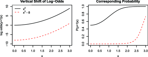
The black and red curves in the left panel of Figure 3 show the conditional log-odds for our misspecified model with two different values of , 0 and , respectively. On the log-odds scale, one is no steeper than the other. But when we look at the same two curves on the conditional probability scale (right panel), now the red looks steeper than the black. This is due to a “ceiling” effect for the black curve: in the region where the log-odds is changing fast, the probability has already saturated at 1. The actual estimates of and depend on the background density of as well as ; see Section 4.5 for a full simulation.
As Warton and Shepherd (2010) prove, this ceiling effect vanishes in the limit where ; in that case , , and the logistic regression and IPP estimates are identical. Hence, there is no difference when the background sample grows so large that it dwarfs the presence records in the population from which we are sampling. Dorazio (2012) considers a similar framework, called the case-augmented design, and proves a similar equivalency to the IPP as .
4.3 Infinitely weighted logistic regression.
If we modify the logistic regression procedure a bit, we can resolve the discrepancy in the previous section and recover the same that we would estimate with an IPP using the same presence and background samples.
We can remove the ceiling effect of the previous section if we add case weights to the samples
| (32) |
for some large number . We then obtain the weighted log-likelihood
| (33) | |||||
| (34) |
Proposition 2
Let be any convex penalty, and suppose has a unique maximizer . Then if maximize for weight ,
| (35) |
Reparameterizing (33) with and ignoring constants, we obtain
Fixing and taking , each term in the second sum converges to while the third sum converges to 0. Hence, ignoring constants, (4.3) converges to the numerical IPP log-likelihood (9), and this convergence occurs uniformly on compact subsets of the parameter space.
Now, both and are concave, and the latter is strictly concave by assumption; hence, the maximizer of the first converges to the maximizer of the second.
From the above, we see that IWLR is not really a new statistical method, but rather a technical device for optimizing the IPP/Maxent log-likelihood using already-implemented GLM software.
Although technically for any finite (hence the name “infinitely weighted”), in practice, we only need large enough that the approximation of to is good near .
Essentially, if for each (say, all are less than 0.001), then the Taylor approximation should be good. We can assess this easily if we observe that
| (37) |
when all of the above are small. To rephrase, then, if from the logistic regression is less than 0.001 or so, it seems to us that should be sufficiently large. If not, we can set and check that the fitted are now small enough. If any uncertainty remains whether is large enough, one can always increase it by (say) another factor of 100 and check that the estimates do not change appreciably.
4.4 Logistic regression as density estimation.
One interpretation of the results we have just reviewed is that in the context of presence-only data, logistic regression solves the same parametric density estimation problem as Maxent and the IPP do. Moreover, our infinitely weighted logistic regression yields an identical estimate of the density.
Using logistic regression for density estimation has been proposed before. For example, Hastie, Tibshirani and Friedman (2009) discuss it as a means for turning an unsupervised density estimation problem into a supervised classification problem. Their proposal uses a different weighting scheme (assigning half the total weight to the presence samples) which, unlike infinitely weighted logistic regression, does not give exactly the IPP solution.
4.5 Simulation study: Weighted vs unweighted logistic regression.
We have seen that both infinitely weighted logistic regression (a.k.a. numerical IPP) and unweighted logistic regression estimate the same parameter of the same log-linear IPP model, and when the background sample is much larger than the presence sample the estimates are close to each other.
However, the infinitely weighted logistic regression estimate can converge much faster to the large-background-sample limit if the linear model is misspecified, as we illustrate here with a simulation study.
Consider a geographic region with a single covariate whose background density is . Now, suppose a species follows our log-linear IPP model with slope , so that . Then the density of presence samples in feature space is .
Suppose our species is in fact a mixture of two subspecies, one of which comprises 95% of the population and prefers large, while the remaining 5% prefer small. If each subspecies follows our model with coefficients 1.5 and , respectively, then
| (38) |
which no longer follows the log-linear model. and are depicted in the upper panel of Figure 4 as the dashed and solid black lines. The black line in the left panel shows , the relative intensity as a function of the covariate . In the left panel all the curves have been normalized so that .
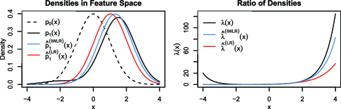
If we fit an infinitely-weighted logistic regression (or, equivalently, a log-linear IPP) to a large presence and background sample, our fitted will tend to . We have plotted the corresponding large-sample estimates and as blue lines in the respective panels of Figure 4.
If, alternatively, we fit an unweighted logistic regression to the same data set with large , the estimate will tend to roughly 1.04. The resulting large-sample estimates and are plotted in red.
If we fit an unweighted logistic regression to a large sample with a different ratio , we would get a different estimate, which would tend toward the IPP estimate of 1.325 if and only if this ratio tended to 0. By the same token, when and are fixed, the ratio between them can play a significant role in determining the estimated . In contrast, the IWLR/IPP estimate tends to 1.325 in large samples no matter what the ratio .
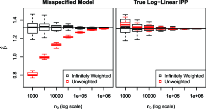
The left panel of Figure 5 illustrates this with a simulation study of the example just discussed. We first generate a single presence sample of size from this species, then generate 20 sets of background samples from for each of a range of values ranging from to .
For each background sample, we fit both an “infinitely” weighted () and unweighted logistic regression to the combination of presence and background points. For relatively large sizes of background sample, there is very little sampling variability, but the logistic regression estimates carry a large bias that depends greatly on the size of the background sample. The limiting , to which both methods would converge given an infinite background sample, is depicted with a horizontal line.
In the right panel, we repeat this study with a presence sample from , the correctly-specified model with the same mean as our misspecified model. Now the situation is very different; no matter what the mix of presence and background samples, the log-odds are truly linear with slope . Consequently, as and , regardless of the limiting ratio .
Since the choice of background sample size is primarily a matter of convenience, it is preferable to use an estimator that depends on it as little as possible. When the linear model is misspecified (which is nearly always the case), we recommend the infinitely weighted logistic regression over unweighted logistic regression for this reason.
We emphasize here that although IWLR resolves the issue of bias that we discussed in Section 4.2, using IWLR does not guarantee that we will obtain a good estimate for small . The smaller is, the larger the variance of our estimate, so a larger background set is always better unless computational constraints apply.
What is more, the variability in our estimate due to the background sample is not reflected in the default standard error outputs from GLM software—only the variability due to the presence records is. Because for large , its Hessian will also converge to the Hessian of the IPP.
Even if our background sample was extremely large, the standard error estimates for any of the models we have discussed are based on asymptotic normal approximations that hold when the log-linear model is correctly specified. Resampling methods such as the bootstrap are more generally reliable, but even the bootstrap will depend crucially on the assumption that presence records (and in the case of logistic regression, background records) are independent observations. In terms of the IPP model, this assumption rules out spatial clustering of presence records. Renner and Warton (2013) provide evidence that this assumption may not hold for presence-only data. Therefore, model-based estimates of standard error should be viewed with suspicion no matter what method we choose.
5 Discussion.
We have discussed several closely related models for a single presence-only sample. In this section we collect them all in one place and review their relationships:
The “mother” model, from which the others can be derived, is the inhomogeneous Poisson process (IPP), whose log-likelihood is
| (39) |
In practice, (39) is approximated numerically via
| (40) |
Fitting this model amounts to solving for the density for which the expected features match the empirical mean , then multiplying that density by .
Conditioning on , we obtain the exponential family density model , resulting in the log-likelihood
| (41) |
or its numerical counterpart. This is the log-likelihood maximized by Maxent, and it corresponds exactly to the log-likelihood (39) partially maximized with respect to . Hence, both procedures give exactly the same estimates of and .
The logistic regression log-likelihood is
| (42) |
When the log-linear IPP model is correctly specified, this model is as well (aside from the fact that the are only approximately independent), with the same true as in the IPP model. However, in finite samples the estimates for given by maximizing (42) instead of (40) may be substantially different.
We can resolve this difference by upweighting all the background points by , obtaining weighted log-likelihood
| (43) |
In the limit where , we recover exactly the same as we would by maximizing (40).
Another means for approximating the IPP log-likelihood with a GLM log-likelihood is the Berman and Turner method, which simply discretizes geographic space into pixels and assigns each presence point to a bin belonging to its nearest background point:
| (44) |
This discretization of presence features is unnecessary given that we can exactly fit the IPP likelihood using the infinitely weighted approach of (43).
5.1 Extending the IPP model.
Logistic regression is one of the most widely applied methods in statistics. For decades, applied statisticians have been developing, studying and using variations on logistic regression to solve classification problems in statistics. R packages exist for fitting generalized additive models (GAMs), boosted regression trees, MARS and every manner of tailored regularization schemes [see, e.g., Hastie, Tibshirani and Friedman (2009)].
All of these methods are well understood within the context of logistic regression. We believe that the most important practical implication of the finite-sample equivalence between the IPP model and infinitely weighted logistic regression is that all of these methods can now be equally well understood and easily applied within the context of the IPP model.
For instance, we can fit an IPP / Maxent version of boosted regression trees with the following single line of R:
boosted.ipp <- gbm(y~., family=‘‘bernoulli,’’
data=dat, weights=1E3^(1-y)).
For an IPP / Maxent version of LASSO, ridge, or the elastic net:777The user should be warned that glmnet automatically re-normalizes the weights so they sum to . To avoid issues, set glmnet.control(pmin=1.0e-8, fdev=0) in your R session, and keep in mind this renormalization when setting the Lagrange parameter .
lasso.ipp <- glmnet(dat.x, dat.y, family=‘‘binomial,’’
weights=1E3^(1-y)).
For an IPP GAM:
gam.ipp <- gam(y~s(x1)+x2, family=binomial, data=dat,
weights=1E3^(1-y)).
This added flexibility promises to provide a powerful tool to modelers of presence-only data.
5.2 Model selection.
Regardless of which of the various related likelihoods we choose, there remains the issue of model selection. With the use of geographic information systems, ecologists often have access to a large number of predictor variables and may wish to winnow the field before modeling to avoid overfitting. Conversely, if some continuous variables are known to be important predictors, assuming a linear effect on the log-intensity may be too restrictive, and we may wish to expand the basis using splines, interactions, wavelets, etc. In either case, regularization may be called for.
Though it would be impossible to give a full treatment here of the many important considerations governing model selection, we note that these choices need not be governed by which likelihood we take as our starting point. In particular, the large set of derived features and regularization used by Maxent software can just as well be applied to the IPP model or, for that matter, to logistic regression. Using the infinitely weighted logistic regression method, we can implement the exact loss function used by the Maxent with software for penalized GLMs.
Acknowledgments.
The authors are grateful to Jane Elith for helpful discussions and suggestions. We were also very fortunate to have had very thorough and thoughtful reviewers; the current manuscript has benefited greatly from their attention.
References
- Aarts, Fieberg and Matthiopoulos (2012) {barticle}[author] \bauthor\bsnmAarts, \bfnmG.\binitsG., \bauthor\bsnmFieberg, \bfnmJ.\binitsJ. and \bauthor\bsnmMatthiopoulos, \bfnmJ.\binitsJ. (\byear2012). \btitleComparative interpretation of count, presence–absence and point methods for species distribution models. \bjournalMethods in Ecology and Evolution \bvolume3 \bpages177–187. \bptokimsref \endbibitem
- Baddeley and Turner (2000) {barticle}[mr] \bauthor\bsnmBaddeley, \bfnmAdrian\binitsA. and \bauthor\bsnmTurner, \bfnmRolf\binitsR. (\byear2000). \btitlePractical maximum pseudolikelihood for spatial point patterns (with discussion). \bjournalAust. N. Z. J. Stat. \bvolume42 \bpages283–322. \biddoi=10.1111/1467-842X.00128, issn=1369-1473, mr=1794056 \bptnotecheck related\bptokimsref \endbibitem
- Baddeley et al. (2010) {barticle}[mr] \bauthor\bsnmBaddeley, \bfnmA.\binitsA., \bauthor\bsnmBerman, \bfnmM.\binitsM., \bauthor\bsnmFisher, \bfnmN. I.\binitsN. I., \bauthor\bsnmHardegen, \bfnmA.\binitsA., \bauthor\bsnmMilne, \bfnmR. K.\binitsR. K., \bauthor\bsnmSchuhmacher, \bfnmD.\binitsD., \bauthor\bsnmShah, \bfnmR.\binitsR. and \bauthor\bsnmTurner, \bfnmR.\binitsR. (\byear2010). \btitleSpatial logistic regression and change-of-support in Poisson point processes. \bjournalElectron. J. Stat. \bvolume4 \bpages1151–1201. \biddoi=10.1214/10-EJS581, issn=1935-7524, mr=2735883 \bptokimsref \endbibitem
- Berman and Turner (1992) {barticle}[author] \bauthor\bsnmBerman, \bfnmM.\binitsM. and \bauthor\bsnmTurner, \bfnmT. R.\binitsT. R. (\byear1992). \btitleApproximating point process likelihoods with GLIM. \bjournalJ. Appl. Stat. \bvolume41 \bpages31–38. \bptokimsref \endbibitem
- Chakraborty et al. (2011) {barticle}[mr] \bauthor\bsnmChakraborty, \bfnmAvishek\binitsA., \bauthor\bsnmGelfand, \bfnmAlan E.\binitsA. E., \bauthor\bsnmWilson, \bfnmAdam M.\binitsA. M., \bauthor\bsnmLatimer, \bfnmAndrew M.\binitsA. M. and \bauthor\bsnmSilander, \bfnmJohn A.\binitsJ. A. (\byear2011). \btitlePoint pattern modelling for degraded presence-only data over large regions. \bjournalJ. R. Stat. Soc. Ser. C. Appl. Stat. \bvolume60 \bpages757–776. \biddoi=10.1111/j.1467-9876.2011.00769.x, issn=0035-9254, mr=2844854 \bptokimsref \endbibitem
- Cressie (1993) {bbook}[mr] \bauthor\bsnmCressie, \bfnmNoel A. C.\binitsN. A. C. (\byear1993). \btitleStatistics for Spatial Data. \bpublisherWiley, \blocationNew York. \bnoteRevised reprint of the 1991 edition. \bidmr=1239641 \bptokimsref \endbibitem
- Dorazio (2012) {barticle}[mr] \bauthor\bsnmDorazio, \bfnmRobert M.\binitsR. M. (\byear2012). \btitlePredicting the geographic distribution of a species from presence-only data subject to detection errors. \bjournalBiometrics \bvolume68 \bpages1303–1312. \biddoi=10.1111/j.1541-0420.2012.01779.x, issn=0006-341X, mr=3040037 \bptokimsref \endbibitem
- Elith et al. (2006) {barticle}[author] \bauthor\bsnmElith, \bfnmJ.\binitsJ., \bauthor\bsnmGraham, \bfnmC. H.\binitsC. H., \bauthor\bsnmAnderson, \bfnmR. P.\binitsR. P., \bauthor\bsnmDudik, \bfnmM.\binitsM., \bauthor\bsnmFerrier, \bfnmS.\binitsS., \bauthor\bsnmGuisan, \bfnmA.\binitsA., \bauthor\bsnmHijmans, \bfnmR. J.\binitsR. J., \bauthor\bsnmHuettmann, \bfnmF.\binitsF., \bauthor\bsnmLeathwick, \bfnmJ. R.\binitsJ. R., \bauthor\bsnmLehmann, \bfnmA.\binitsA. \betalet al. (\byear2006). \btitleNovel methods improve prediction of species’ distributions from occurrence data. \bjournalEcography \bvolume29 \bpages129–151. \bptokimsref \endbibitem
- Elith et al. (2011) {barticle}[author] \bauthor\bsnmElith, \bfnmJ.\binitsJ., \bauthor\bsnmPhillips, \bfnmS. J.\binitsS. J., \bauthor\bsnmHastie, \bfnmT.\binitsT., \bauthor\bsnmDudík, \bfnmM.\binitsM., \bauthor\bsnmChee, \bfnmY. E.\binitsY. E. and \bauthor\bsnmYates, \bfnmC. J.\binitsC. J. (\byear2011). \btitleA statistical explanation of MaxEnt for ecologists. \bjournalDiversity and Distributions \bvolume17 \bpages43–57. \bptokimsref \endbibitem
- Gaetan and Guyon (2009) {bbook}[author] \bauthor\bsnmGaetan, \bfnmC.\binitsC. and \bauthor\bsnmGuyon, \bfnmX.\binitsX. (\byear2009). \btitleSpatial Statistics and Modeling. \bpublisherSpringer, \blocationNew York. \bptokimsref \endbibitem
- Hastie, Tibshirani and Friedman (2009) {bbook}[mr] \bauthor\bsnmHastie, \bfnmTrevor\binitsT., \bauthor\bsnmTibshirani, \bfnmRobert\binitsR. and \bauthor\bsnmFriedman, \bfnmJerome\binitsJ. (\byear2009). \btitleThe Elements of Statistical Learning: Data Mining, Inference, and Prediction, \bedition2nd ed. \bpublisherSpringer, \blocationNew York. \biddoi=10.1007/978-0-387-84858-7, mr=2722294 \bptokimsref \endbibitem
- Johnson et al. (2006) {barticle}[author] \bauthor\bsnmJohnson, \bfnmChris J.\binitsC. J., \bauthor\bsnmNielsen, \bfnmScott E.\binitsS. E., \bauthor\bsnmMerrill, \bfnmEvelyn H.\binitsE. H., \bauthor\bsnmMcDonald, \bfnmTrent L.\binitsT. L. and \bauthor\bsnmBoyce, \bfnmMark S.\binitsM. S. (\byear2006). \btitleResource selection functions based on use-availability data: Theoretical motivation and evaluation methods. \bjournalJournal of Wildlife Management \bvolume70 \bpages347–357. \bptokimsref \endbibitem
- Lee, Scott and Wild (2006) {barticle}[mr] \bauthor\bsnmLee, \bfnmA. J.\binitsA. J., \bauthor\bsnmScott, \bfnmA. J.\binitsA. J. and \bauthor\bsnmWild, \bfnmC. J.\binitsC. J. (\byear2006). \btitleFitting binary regression models with case-augmented samples. \bjournalBiometrika \bvolume93 \bpages385–397. \biddoi=10.1093/biomet/93.2.385, issn=0006-3444, mr=2278091 \bptokimsref \endbibitem
- Lele and Keim (2006) {barticle}[pbm] \bauthor\bsnmLele, \bfnmSubhash R.\binitsS. R. and \bauthor\bsnmKeim, \bfnmJonah L.\binitsJ. L. (\byear2006). \btitleWeighted distributions and estimation of resource selection probability functions. \bjournalEcology \bvolume87 \bpages3021–3028. \bidissn=0012-9658, pmid=17249227 \bptokimsref \endbibitem
- MacKenzie (2006) {bbook}[author] \bauthor\bsnmMacKenzie, \bfnmDarryl I.\binitsD. I. (\byear2006). \btitleOccupancy Estimation and Modeling: Inferring Patterns and Dynamics of Species Occurrence. \bpublisherAcademic Press, \blocationNew York. \bptokimsref \endbibitem
- Manly et al. (2002) {bbook}[author] \bauthor\bsnmManly, \bfnmB. F. J.\binitsB. F. J., \bauthor\bsnmMcDonald, \bfnmL. L.\binitsL. L., \bauthor\bsnmThomas, \bfnmD. L.\binitsD. L., \bauthor\bsnmMcDonald, \bfnmT. L.\binitsT. L. and \bauthor\bsnmErickson, \bfnmW. P.\binitsW. P. (\byear2002). \btitleResource Selection by Animals: Statistical Analysis and Design for Field Studies. \bpublisherKluwer Academic, \blocationDordrecht. \bptokimsref \endbibitem
- Margules et al. (1994) {barticle}[author] \bauthor\bsnmMargules, \bfnmC. R.\binitsC. R., \bauthor\bsnmAustin, \bfnmM. P.\binitsM. P., \bauthor\bsnmMollison, \bfnmD.\binitsD. and \bauthor\bsnmSmith, \bfnmF.\binitsF. (\byear1994). \btitleBiological models for monitoring species decline: The construction and use of data bases (with discussion). \bjournalPhilosophical Transactions of the Royal Society of London. Series B: Biological Sciences \bvolume344 \bpages69–75. \bptokimsref \endbibitem
- Phillips, Anderson and Schapire (2006) {barticle}[author] \bauthor\bsnmPhillips, \bfnmS. J.\binitsS. J., \bauthor\bsnmAnderson, \bfnmR. P.\binitsR. P. and \bauthor\bsnmSchapire, \bfnmR. E.\binitsR. E. (\byear2006). \btitleMaximum entropy modeling of species geographic distributions. \bjournalEcological Modelling \bvolume190 \bpages231–259. \bptokimsref \endbibitem
- Phillips, Dudík and Schapire (2004) {binproceedings}[author] \bauthor\bsnmPhillips, \bfnmS. J.\binitsS. J., \bauthor\bsnmDudík, \bfnmM.\binitsM. and \bauthor\bsnmSchapire, \bfnmR. E.\binitsR. E. (\byear2004). \btitleA maximum entropy approach to species distribution modeling. In \bbooktitleProceedings of the Twenty-First International Conference on Machine Learning \bpages83. \bpublisherACM, \blocationNew York. \bptokimsref \endbibitem
- Phillips and Dudík (2008) {barticle}[author] \bauthor\bsnmPhillips, \bfnmS. J.\binitsS. J. and \bauthor\bsnmDudík, \bfnmM.\binitsM. (\byear2008). \btitleModeling of species distributions with Maxent: New extensions and a comprehensive evaluation. \bjournalEcography \bvolume31 \bpages161–175. \bptokimsref \endbibitem
- Phillips and Elith (2013) {barticle}[pbm] \bauthor\bsnmPhillips, \bfnmSteven J.\binitsS. J. and \bauthor\bsnmElith, \bfnmJane\binitsJ. (\byear2013). \btitleOn estimating probability of presence from use-availability or presence-background data. \bjournalEcology \bvolume94 \bpages1409–1419. \bidissn=0012-9658, pmid=23923504 \bptokimsref \endbibitem
- Renner and Warton (2013) {barticle}[pbm] \bauthor\bsnmRenner, \bfnmIan W.\binitsI. W. and \bauthor\bsnmWarton, \bfnmDavid I.\binitsD. I. (\byear2013). \btitleEquivalence of MAXENT and Poisson point process models for species distribution modeling in ecology. \bjournalBiometrics \bvolume69 \bpages274–281. \biddoi=10.1111/j.1541-0420.2012.01824.x, issn=1541-0420, pmid=23379623 \bptokimsref \endbibitem
- Royle, Nichols and Kéry (2005) {barticle}[author] \bauthor\bsnmRoyle, \bfnmJ. Andrew\binitsJ. A., \bauthor\bsnmNichols, \bfnmJames D.\binitsJ. D. and \bauthor\bsnmKéry, \bfnmMarc\binitsM. (\byear2005). \btitleModelling occurrence and abundance of species when detection is imperfect. \bjournalOikos \bvolume110 \bpages353–359. \bptokimsref \endbibitem
- Ward et al. (2009) {barticle}[mr] \bauthor\bsnmWard, \bfnmGill\binitsG., \bauthor\bsnmHastie, \bfnmTrevor\binitsT., \bauthor\bsnmBarry, \bfnmSimon\binitsS., \bauthor\bsnmElith, \bfnmJane\binitsJ. and \bauthor\bsnmLeathwick, \bfnmJohn R.\binitsJ. R. (\byear2009). \btitlePresence-only data and the EM algorithm. \bjournalBiometrics \bvolume65 \bpages554–563. \biddoi=10.1111/j.1541-0420.2008.01116.x, issn=0006-341X, mr=2751480 \bptokimsref \endbibitem
- Warton and Shepherd (2010) {barticle}[mr] \bauthor\bsnmWarton, \bfnmDavid I.\binitsD. I. and \bauthor\bsnmShepherd, \bfnmLeah C.\binitsL. C. (\byear2010). \btitlePoisson point process models solve the “pseudo-absence problem” for presence-only data in ecology. \bjournalAnn. Appl. Stat. \bvolume4 \bpages1383–1402. \biddoi=10.1214/10-AOAS331, issn=1932-6157, mr=2758333 \bptokimsref \endbibitem
- Xie and Manski (1989) {barticle}[author] \bauthor\bsnmXie, \bfnmYu\binitsY. and \bauthor\bsnmManski, \bfnmCharles F.\binitsC. F. (\byear1989). \btitleThe logit model and response-based samples. \bjournalSociol. Methods Res. \bvolume17 \bpages283–302. \bptokimsref \endbibitem