A Robust Relay Placement Framework for 60GHz mmWave Wireless Personal Area Networks

Abstract

Multimedia streaming applications with stringent QoS requirements in 60GHz mmWave wireless personal area networks (WPANs) demand high rate and low latency data transfer as well as low service disruption. In this paper, we consider the problem of robust relay placement in 60GHz WPANs. Relays forward traffic from transmitter devices to receiver devices facilitating i) the primary communication path for non-line-of-sight (NLOS) transceiver pairs, and ii) secondary (backup) communication path for line-of-sight (LOS) transceiver pairs. We formulate the robust minimum relay placement problem and the robust maximum utility relay placement problem with the objective to minimize the number of relays deployed and maximize the network utility, respectively. Efficient algorithms are developed to solve both problems and have been shown to incur less service disruption in presence of moving subjects that may block the LOS paths in the environment.

I Introduction

The millimeter wave (mmWave) band has attracted considerable commercial interests due to the advance in low-cost mmWave radio frequency integrated circuit design. The mmWave band provides 7GHz unlicensed spectrum resource at the center frequency of 60GHz (57-64GHz in North America, and 59-66GHz in Europe and Japan), which would enable many high data rate applications like high definition streaming multimedia, high-speed kiosk data transfer and point-to-point terminal communication in data center [1, 2, 3], etc.

In contrast to many existing RF technologies such as 2.4GHz WiFi radios, mmWave radio has several unique physical characteristics. First, the propagation and attenuation loss are much more severe in 60GHz band. It is shown that the free space path loss in 60GHz is more than 20dB larger than that in 5GHz. The oxygen absorption loss is as high as 5-30dB/km. Furthermore, the penetration loss is also much higher through typical building materials [1]. As a result, line-of-sight (LOS) path is the predominant path for signal transmission, while signals along the second-order and higher-order reflection paths are significantly attenuated and often negligible. Second, to combat such severe signal degradation, directional antenna technology is essential in mmWave devices. By using directional antennae on both the transmitter and the receiver sides, mmWave radios can obtain significant gain in the received signal strength, while incurring negligible interference to/from other mmWave devices [4, 5, 6]. In this paper, we consider an mmWave wireless personal area network (WPANs) equipped with directional antennae on all devices.

In addition to high bandwidth demands, multimedia applications in 60GHz WPANs also have stringent requirements on service disruption (defined as the frequency and duration of time that network connectivity is not available), which can occur due to changes in channel conditions such as LOS link blockage by moving subjects in the space. This motivates us to employ relays for two purposes. First, relays can be used to forward traffic from transmitters to receivers that do not have LOS connectivity. Second, relays can provide a secondary (2-hop) path in case of blockage on the primary (direct) path.

Generally, there are two types of relays proposed for mmWave in the literature, active relay [7, 8, 9] and passive relay [10, 11, 12]. A passive relay (also known as reflector) reflects the mmWave radiation from transmitter to receiver. It can be as simple as a flat metal plate that does not require any power source. However, it introduces losses due to reflection, as well as the additional path loss as a result of longer propagation path. In contrast, an active relay is an active mmWave transceiver with beamforming capabilities. It can amplify and forward the mmWave signal from the transmitter to any intended direction, at the cost of higher complexity and maintenance. In this paper, we consider active relays for the ease of control of reflection directions and signal boost.

In this paper, two relay placement problems in 60GHz mmWave WPANs are investigated: robust minimum relay placement (RMRP) that attempts to find the minimum number of relays and their best placements from a set of candidate locations with bandwidth and robustness constraints, and robust maximum utility relay placement (RMURP) that aims to maximize network utility given a fixed number of relays. Two vertex-disjoint (except for the endpoints) paths (one called the primary path, and the other the secondary path) are provisioned between each pair of transmitter and receiver. Consequently, seamless switching to the secondary path is facilitated in event of channel degradation or blockage on the primary path avoiding service disruption. Robustness is characterized by the D-norm uncertainty model, which models tolerance to concurrent (worst-case) failures of a subset of primary paths[13]. Using linear relaxation and the duality theorem of linear programming, RMRP and RMURP are transformed to the mixed integer linear programming (MILP) and mixed integer non-linear programming (MINLP) problems, respectively. Two algorithms, bisector search and Generalized Benders Decomposition, are proposed for RMURP and are shown to have near optimal and optimal performance. Extensive simulations demonstrate the fault tolerance of the proposed relay placement algorithms in significantly reducing the probability of service disruption.

The rest of this paper is organized as follows. The related literature work is analyzed in Section II. In Section III, we introduce the network model and the problem statements for robust relay placement. The RMRP formulation is presented in Section IV, while RMURP is formulated in a similar way in Section V. Furthermore, we also discuss two proposed algorithms for RMURP in Section V. Performance evaluation is presented in Section VI. Finally, we conclude this paper in Section VII.

II Related Work

Significant prior literature have been produced on different aspects of 60GHz radios, from CMOS circuit design to network protocol development. In this section, we summarize prior work on MAC design in mmWave WPANs.

A spatial time-division multiple access (STDMA) scheme was proposed for a realistic multi-Gbps mmWave WPAN in [14]. With the help of a heuristic scheduling algorithm, it is able to achieve significant throughput enhancement as much as 100% compared to conventional TDMA schedules. In [15], Cai et al. presented an efficient resource management framework based on the unique physical characteristics in a MC-DS-CDMA based mmWave networks. The authors also conducted extensive analysis of spatial multiplexing capacity in mmWave WPANs with directional antennae in [16, 17]. In [5], Madhow et al. conducted a probabilistic analysis of the interference in an mmWave network, as the result of uncoordinated transmission. It is concluded that an mmWave link can be abstracted as a “pseudo-wired link” with negligible interference when the beam width is 20 degree. Similar observations are made in [18, 4]. Therefore, the primary interference at the transmitter or receiver devices is the predominant source of contention. In [19, 20], to address the deafness problem induced by directionality, Gong et al. proposed a new directional CSMA/CA protocol for IEEE 802.15.3c 60GHz WPANs. With virtual carrier sensing, the central coordinator can distribute the network allocation vector (NAV) information, to avoid collisions among the devices occupying the same channel. The author also extended the work to a multiple-user scenario in [21]. A distributed scheduling protocol is proposed by coordinating mmWave mesh nodes in [6], and can achieve high resource utilization with time division multiplexing (TDM). However, none of the above work model or address relay placement problems in mmWave WPANs with directional antennae.

There are also some existing work on repeater selection and relay operation scheduling in mmWave WPANs. Repeater selection was investigated in [8], with the objective to maximize data rate for each transmitter and receiver pair by determining the best link allocation. In [22], Lan et al. explored time slot scheduling for relay operations in the scenario of directional antenna on mmWave devices and formulated the throughput maximization problem as an integer programming problem. However, both schemes do not consider robustness in presence of uncertain link blockage.

Our work is also related to multihop routing in wireless networks with directional antenna [23, 24, 25] with two key differences. First, relays in our work are dedicated devices that do not generate or receive application layer packets. Second, we allow at most 2-hop paths between any mmWave transmitter-receiver pair, considering the fact that mmWave WPANs are deployed in small indoor environment with stringent QoS requirement.

To the best of our knowledge, we are the first to explore robust relay placement in 60GHz WPANs. Some preliminary results are presented in [26].

III Network Model and Problem Statement

Consider an mmWave network consisting of a set of $L$ logical mmWave links (simplified as logical links), each link $i\in L$ is associated with a source device (transmitter) $s_{i}$, a destination device (receiver) $d_{i}$, and a traffic demand $r_{i}$ bps. mmWave relay devices (simplified as relays) equipped with steerable antennae can relay data between the transmitters and receivers. The relays can be placed at a set of $K$ candidate locations. We further consider a set of $O$ obstacles in the environment with known locations.

III-A Geometric Model for Link Connectivity

In this section, we introduce a geometric model to characterize link connectivity in 60GHz mmWave WPANs. LOS transmissions are feasible between a transmitter and a receiver if and only if the direct path between them is unobstructed and their distance is less than a threshold $d$.

To bound the end-to-end latency, at most two-hop paths (involving one relay) are allowed between any transmitter-receiver pair. The proposed solutions can be extended to cases where longer paths are allows. Thus, the connectivity of any logical link is determined by the visibility regions of its end points defined as follows:

Definition 1

(Visibility region) Given a 2-D plane of interest, any two points $(a,b)$ are visible to each other if the line segment between them does not intersect with any obstacles and the distance of $a$ and $b$ is no more than $d$. The visibility region $V(a)$ of a point $a$ in the plane is the bounded shape consisting of all unobstructed points no more than distance $d$ from $a$.

Consider transmitter and receiver $a$ and $b$, the (binary) connectivity of logical link $(a,b)$ is thus characterized by:

$$\lambda(a,b)=\begin{cases}1,&\text{iff }V(a)\cap V(b)\neq\varnothing\\ 0,&\text{otherwise }\end{cases},$$ (1)

If $\lambda(a,b)=1$, logical link $(a,b)$ is feasible (directly or via a relay in $a$ and $b$’s overlapping visibility region); otherwise, it is infeasible. For the rest of the paper, we only consider the set of feasible logical links given by:

$$\Omega=\{i\mid\lambda(s_{i},d_{i})=1,\forall i\in L\},$$ (2)

where $s_{i}$, $d_{i}$ are the transmitter and receiver of the $i$-th logical link respectively.

Fig. 1 illustrates the notion of visibility region. There are two mmWave end devices, DEV1 and DEV2. The shadowed area corresponds to the overlapped visibility region between DEV1 and DEV2, which is the candidate region for relay placement for DEV1 and DEV2. The existence of overlapped visibility region is the necessary and sufficient condition of the connectivity of logical links, in both LOS and non-LOS (NLOS) cases.

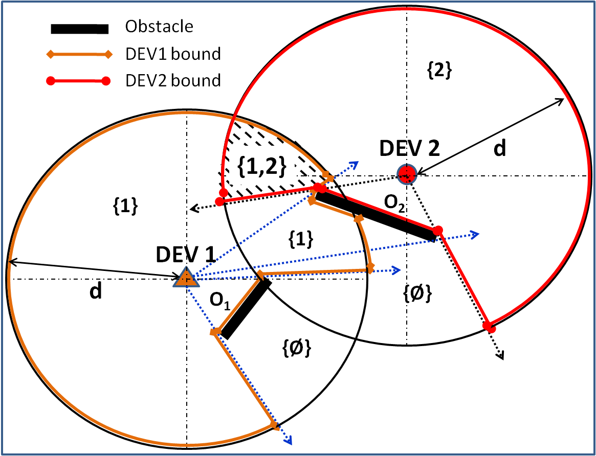
Figure 1: Visibility region and overlapped visibility region.

The relationship between feasible logical links and candidate relay locations can be modeled as an undirected bi-partite graph $G(\Omega,\mathcal{K},E)$, where $\mathcal{K}={1,\ldots,K}$ is the set of candidate relay locations. An edge $e=(l,k)$ exists between a logical link $l\in\Omega$ and a candidate relay location $k\in\mathcal{K}$ iff $k$ is in $V(s_{l})\cap V(d_{l})$, where $s_{l}$ and $d_{l}$ are the end points of $l$. Thus, the set of feasible logical links that can use a relay placed at the candidate location $k$ as relay is given by:

$$\Omega_{k}=\{i\mid k\in V(s_{i})\cap V(d_{i}),\forall i\in\Omega\},\forall k\in\mathcal{K}.\\$$ (3)

III-B Needs for robustness

Relays serve two purposes: i) providing the primary communication path for NLOS logical links; and ii) providing secondary (backup) communication path for LOS or NLOS logical links. Provisioning of secondary paths reduces service disruption when the primary path is obstructed.

To see the impact of secondary paths, we conduct a simple simulation study. Consider a home-network environment in Fig. 2(a), where there is a LOS logical link $l$ and a dedicated relay at a fixed location. In the robust setting, one relay is used to provide a secondary communication path for $l$. Inside the room, there are $M$ moving human subjects modeled as a circle with a radius of 0.3 meters. We adopt a classic random walk model [27], where in each step, a person moves 0.3 meters with the direction randomly chosen from the set $\{-90^{o},-45^{o},0^{o},45^{o},90^{o}\}$. Without relays, the communication between TX and RX is disrupted when a person blocks the direct LOS path. With relays, an outage occurs only when both the primary (LOS) path and the secondary path (via the relay) are blocked. Fig. 2(b) and Fig. 2(c) show the percentage of link blockage and the mean blockage duration with 90% confidence interval versus different number of moving human subjects, respectively.

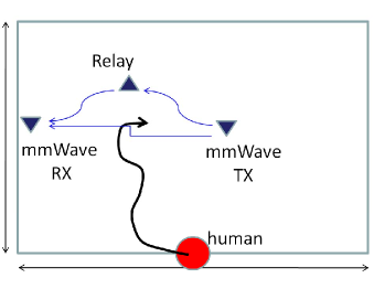
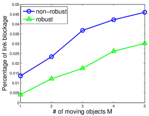
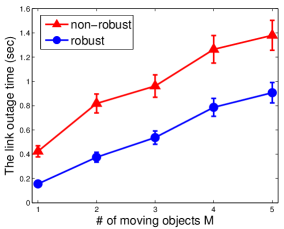
(a) Simulation setup	(b) Percentage of link blockage	(c) Mean blockage duration with 90% confidence interval

Figure 2: Link blockage with and without relay due to moving human subjects in a 10m $\times$ 10m room with a fixed mmWave TX/RX and a dedicated relay, $M$ human subjects moving randomly inside.

As shown in Fig. 2 (b)(c), when the number of moving subjects increases, the percentage of link blockage and blockage duration increase with and without the secondary path. However, the use of backup path reduces both the blocking probability and the duration of each outage. This translates to better quality of service (QoS) at the application layer.

III-C Problem Statement

Relay placement concerns with the selection of relays among a finite set of candidate locations to optimize for certain network utilities. We consider two variations of the problem.

Definition 2

(Robust Minimum Relay Placement (RMRP) problem) Given an mmWave network with a set of feasible logical links with fixed traffic demands, find the minimum number of relays and their locations among candidate location set $\mathcal{K}$ that satisfy connectivity, bandwidth and robustness constraints.

Definition 3

(Robust Maximum Utility Relay Placement (RMURP) problem) Given an mmWave network with a set of feasible logical links with base traffic demands, find the placement of at most $m$ relays among candidate location set $\mathcal{K}$ such that the ratio of the achievable rates over the base rate is maximized subject to robustness constraints.

We restrict the relay of data to relays only. In the robust formulation, for each feasible logical link, two vertex-disjoint (except for the endpoints) communication paths are provisioned, one as primary path, and the other as secondary path. Both the primary and secondary paths between mmWave transmitters and receivers cannot be more than 2-hops. If a relay serves as relay for more than one logical links, time division medium access (TDMA) scheduling is adopted. The interference among concurrent transmissions is assumed to negligible due to the high directionality of mmWave communications, which is consistent with the measurement results reported in [6]. Therefore, the main sources of contention arise from the half-duplex constraint and multiplexing at the relay nodes.

IV Robust Minimum Relay Placement (RMRP)

In this section, we present the analytical form of the RMRP problem. The following notations are used:

• Primary indicator: $x_{ik}=1$ if relay $k$ is selected by logical link $i$ as its primary path relay; otherwise, $x_{ik}=0$;

• Secondary indicator: $y_{ik}=1$ if relay $k$ is selected by logical link $i$ as its secondary path relay; otherwise, $y_{ik}=0$;

• Selection indicator: $z_{k}=1$ if relay $k$ is selected by at least one logical link; otherwise, $z_{k}=0$.

• NLOS indicator: $\eta_{i}=1$ if logical link $i$ does not have a LOS path; otherwise, $\eta_{i}=0$.

If a logical link $i$ has a LOS path, no relay is needed for the primary path; otherwise, one relay should be selected for the primary path, which should satisfy the following condition:

$$\sum_{k=1}^{K}x_{ik}=\eta_{i},\forall i\in\Omega.$$ (4)

On the other hand, at least one relay is needed to facilitate the secondary path, that is,

$$\sum_{k=1}^{K}y_{ik}=1,\forall i\in\Omega.$$ (5)

In addition, a relay cannot be used for the primary path and the secondary path simultaneously. Therefore, we have:

$$x_{ik}+y_{ik}\leq 1,\forall i\in\Omega_{k},\forall k.$$ (6)

As mentioned before, for simplicity, we assume each relay has only one half-duplex transceiver. Therefore, the transmission time of relaying a unit data of logical link $i$ via relay $k$ is

$$\tau_{ik}=\frac{1}{R_{s_{i},k}}+\frac{1}{R_{k,d_{i}}},$$ (7)

where $R_{s_{i},k}$, $R_{k,d_{i}}$ are the mmWave data bandwidth between the source and the relay, and between the relay and the destination, respectively. For the AWGN channel, they can be modeled as:

$$R_{s_{i},k}=\begin{cases}&W\log\left[1+\frac{P_{t}G_{t}G_{r}}{P_{n}D(s_{i},k)^{\gamma}}\right]\mbox{ (when $D(s_{i},k)\leq\Theta$)}\\ &0\mbox{ (when $D(k,d_{i})>\Theta$),}\end{cases}$$ (8)

and

$$R_{k,d_{i}}=\begin{cases}&W\log\left[1+\frac{P_{t}G_{t}G_{r}}{P_{n}D(k,d_{i})^{\gamma}}\right]\mbox{ (when $D(k,d_{i})\leq\Theta$)}\\ &0\mbox{ (when $D(k,d_{i})>\Theta$),}\end{cases}$$ (9)

respectively, where $W$ is the channel bandwidth in Hz, $P_{t}$ is the transmission power, $P_{n}$ is the noise floor level, $G_{t}$, $G_{r}$ are transmitter and receiver antenna gains, $\gamma$ is the large-scale path loss index, $D(a,b)$ is the distance from $a$ to $b$, and $\Theta$ is a constant threshold on communications radius.

For a relay $k$, the TDMA scheduling for the associated logical links should satisfy:

$$\sum_{i\in\Omega_{k}}\eta_{i}x_{ik}r_{i}\tau_{ik}+g_{k}(\mathbf{y_{k}},\mathbf{r})\leq z_{k},\forall k,$$ (10)

where $r_{i}$ is the traffic demand of logical link $i$, $\tau_{ik}$ is the unit data relay time of $i$ via relay $k$. The first term on the left side represents the percentage of relay capacity occupied by all the logical links using this relay as their primary path relay. The second term represents the protection function for the set of logical links using this relay as their secondary path relay. A protection function $g_{k}(.)$ measures the robustness of an mmWave WPAN. Its meaning will be further explained in Section IV-A.

To this end, the RMRP problem can be formally stated as:

$$\underset{\mathbf{x,y,z}}{\text{minimize}} \sum_{k}z_{k}$$ (11)

subject to $$\text{Constraints }\eqref{eq5_x}-\eqref{scheduling}$$

variables $$x_{ik},y_{ik},z_{k}\in\{0,1\},\forall i\in\Omega,k=1,\ldots,K$$

IV-A Reformulation under the $D$-norm uncertainty model

Several uncertainty models have been proposed in literature, including General Polyhedron, $D$-norm, Ellipsoid, etc [13]. In this paper, we adopt the $D$-norm uncertainty model that is characterized by the following protection function:

$$g_{k}(\mathbf{y_{k}},\mathbf{r})=\underset{S_{k}:S_{k}\subseteq\Omega_{k},\mid S_{k}\mid=\Gamma_{k}}{\text{max }}\sum_{i\in S_{k}}y_{ik}r_{i}\tau_{ik}.$$ (12)

Under the $D$-norm uncertainty model, among the set of logical links $\Omega_{k}$ that can relay through relay $k$, at most $\Gamma_{k}$ links will be blocked simultaneously on the primary path and consequently transmit on their secondary path via relay $k$. The maximization gives the worst case traffic loads induced on the relay.

Two special cases are of particular interest. If $\Gamma_{k}=|\Omega_{k}|$, then $g_{k}(\mathbf{y_{k}},\mathbf{r})=\sum_{i\in\Omega_{k}}y_{ik}r_{i}\tau_{ik}$. This means all logical links in $\Omega_{k}$ fail simultaneously. This corresponds to the maximum robustness. In this case, more relays may be needed. At the other extreme, if $\Gamma_{k}=0$, no logical link is blocked. Fewer relays are in use. However, there is little fault tolerance in the resulting relay placement. Denote $\rho\equiv\Gamma_{k}/|\Omega_{k}|$ the robustness index. $\rho$ is a parameter to tradeoff between robustness and resource usage.

Under the above $D$-norm uncertainty model, (10) can be rewritten as:

$$\sum_{i\in\Omega_{k}}\eta_{i}x_{ik}r_{i}\tau_{ik}+\underset{S_{k}:S_{k}\subseteq\Omega_{k},\mid S_{k}\mid=\Gamma_{k}}{\text{max }}\sum_{i\in S_{k}}y_{ik}r_{i}\tau_{ik}\leq z_{k},\forall k,$$ (13)

(13) is not directly tractable since it involves an inner-optimization in the protection function. The protection function can be reformulated an integer linear programming problem as follows [13]:

$$\underset{\{0\leq s_{ik}\leq 1\}_{\forall i\in\Omega_{k}}}{\text{max}}\sum_{i\in\Omega_{k}}y_{ik}r_{i}\tau_{ik}s_{ik},$$

$$\text{s.t. }\sum_{i\in\Omega_{k}}s_{ik}\leq\Gamma_{k},$$ (14)

$$s_{ik}\in\{0,1\},\forall i\in\Omega_{k}$$

Consider a linear relaxation of the above problem where $s_{ik}\in[0,1]$. Due to the linearity of the constraints, the optimal solution occurs at the vertices of the feasibility region. Hence the optimal solution $s_{ik}^{*}$ must be either $0$ or $1$, as there is no gap between the integer linear programming and the linear programming solutions.

Taking the dual of the linear programming problem (IV-A), we have:

$$\underset{\{p_{ik}\geq 0\}_{\forall i\in\Omega_{k}},q_{k}\geq 0}{\text{min}}q_{k}\Gamma_{k}+\sum_{i\in\Omega_{k}}p_{ik},$$

$$\text{s.t. }q_{k}+p_{ik}\geq y_{ik}r_{i}\tau_{ik},$$ (15)

Substituting (IV-A) into (11), we can obtain the equivalent formulation of the RMRP problem as a mixed integer linear programming (MILP) problem as follows:

$$\underset{\mathbf{x,y,z,p,q}}{\text{min}} \sum_{k}z_{k}$$ (16)

s.t. $$\sum_{i\in\Omega_{k}}\eta_{i}x_{ik}r_{i}\tau_{ik}+q_{k}\Gamma_{k}+\sum_{i\in\Omega_{k}}p_{ik}\leq z_{k},\;\forall k$$

$$q_{k}+p_{ik}\geq y_{ik}r_{i}\tau_{ik},\;\forall i\in\Omega_{k},\forall k$$

$$\text{Constraints }\eqref{eq5_x}\eqref{eq5_y}\eqref{unique_ref}\eqref{tx_time}\eqref{rate_sr}\eqref{rate_rd}$$

variables $$x_{ik},y_{ik},z_{k}\in\{0,1\},p_{ik}\geq 0,q_{k}\geq 0$$

IV-B Hardness of RMRP

We prove in Appendix -A that RMRP is NP-hard.

The MILP problem in (16) can be solved by any MILP solver. In our implementation, we adopt the MILP solver of the IBM optimization tool – CPLEX [28].

V Robust Maximum Utility Relay Placement (RMURP)

In contrast to RMRP, which tries to minimize the number of relays, RMURP aims to maximize the total utility of an mmWave WPAN given a fixed number of relays.

Let $r_{i}$ be the base traffic demand on logical link $i$. We allow $r_{i}$ be scaled up/down according to network constraints. That is, the actual data rate supported is $\alpha r_{i}$, where $\alpha$ is a scaling parameter. This formulation is particularly relevant for transferring multimedia content that allows adaptive encoding. The objective of RMURP is henceforth to maximize the total utility $U$ of the network, given by $U=\sum_{i}\alpha r_{i}$.

The constraints of RMURP are similar to those of RMRP, except that the TDMA schedulability constraint (10) now becomes

$$\sum_{i\in\Omega_{k}}\eta_{i}x_{ik}\alpha r_{i}\tau_{ik}+g_{k}(\mathbf{y_{k}},\alpha\mathbf{r})\leq z_{k},\forall k,$$ (17)

and the additional cardinality constraint needs to be included:

$$\sum_{k}z_{k}\leq m,$$ (18)

where $m$ is the maximum number of relays to be used.

To this end, the RMURP can be formalized as:

$$\underset{\mathbf{x,y,z,\alpha}}{\text{maximize}} \sum_{i}\alpha r_{i}$$ (19)

subject to $$\text{Constraints }\eqref{eq5_x}\eqref{eq5_y}\eqref{unique_ref}\eqref{tx_time}\eqref{rate_sr}\eqref{rate_rd}\eqref{scheduling_rmurp}\eqref{cardinality}$$

variables $$x_{ik},y_{ik},z_{k}\in\{0,1\},\alpha\geq 0,\forall i,k$$

V-A Reformulation under $D$-norm Uncertainty Model

Again we can apply the $D$-norm uncertainty model (see Section IV-A) to the RMURP problem of (19). This will transform (19) into a mixed integer non-linear programming problem (MINLP) as follows:

$$\underset{\mathbf{x,y,z,p,q,\alpha}}{\text{Maximize}} \sum_{i}\alpha r_{i}$$ (20)

subject to $$\sum_{i\in\Omega_{k}}\eta_{i}x_{ik}\alpha r_{i}\tau_{ik}+q_{k}\Gamma_{k}+\sum_{i\in\Omega_{k}}p_{ik}\leq z_{k},\;\forall k$$

$$q_{k}+p_{ik}\geq y_{ik}\alpha r_{i}\tau_{ik},\;\forall i\in\Omega_{k},\forall k$$

$$\text{Constraints }\eqref{eq5_x}\eqref{eq5_y}\eqref{unique_ref}\eqref{tx_time}\eqref{rate_sr}\eqref{rate_rd}\eqref{cardinality}$$

variables $$x_{ik},y_{ik},z_{k}\in\{0,1\},p_{ik}\geq 0,q_{k}\geq 0,\alpha\geq 0$$

V-B Hardness of RMURP

We prove in Appendix -B that RMURP is NP-hard. The inclusion of variable $\alpha$ renders RMURP an MINLP. Specialized algorithms need to be designed.

Next, we propose two algorithms to solve the RMURP. The first algorithm is based on Bisection Search, which is shown to be fast but does not guarantee optimality. The second algorithm is based on the Generalized Benders’ Decomposition (GBD) technique [29, 30], which is proven to converge to optimal solutions but has higher computation complexity.

V-C Bisection Search

Bisection Search is a heuristic method for finding roots of an equation. It iteratively bisects an interval and then selects the subinterval where a root must reside for the next iteration, until some termination condition is met. It is guaranteed to converge to a root of $f(\cdot)$ if and only if: $f$ is a continuous function on the interval $[A,B]$, and $f(A)$ and $f(B)$ have opposite signs.

In (20), if $\alpha$ is given, RMURP becomes a MILP, which can be solved by CPLEX. The key is thus to determine the value of $\alpha$. When $\alpha$ is large, RMURP is infeasible. When $\alpha=0$, RMURP is always feasible. More generally, if $\alpha_{1}>\alpha_{2}$, RMURP is infeasible when $\alpha=\alpha_{1}$, then, RMURP is feasible when $\alpha=\alpha_{2}$. Treating feasibility and infeasibility as opposite signs, we apply the Bisection Search principle to decide the range of $\alpha$ iteratively until it is smaller than a threshold $2\times TOL$. Starting from an initial interval $[A,B]$, where $\alpha=A$ renders RMURP feasible and $\alpha=B$ renders RMURP infeasible, we substitute A or B with $\frac{A+B}{2}$ depending on the feasibility of RMURP under $\alpha=\frac{A+B}{2}$. The “monotonicity” in the feasibility of RMURP with respective to $\alpha$ makes the Bisection Search converge fast but the optimality of the final results depends on $TOL$.

The Bisection Search based algorithm is summarized in Algorithm 1.

Input : Base logical data rate $r_{i}$ for each feasible logical link $i$; error tolerance $TOL$ (which serves as the iteration termination condition); and the up-to-date known range for $\alpha$: [$A$, $B$]

Output : Maximum network utility $U_{T}$ and relay selection variables for every feasible links $\mathbf{x,y,z}$

begin

       Set $n=1$;

       while $n\leq maxN$ do

             $C\longleftarrow\frac{(A+B)}{2}$;

             Solve the MILP problem $RMURP(C)$.

             if $RMURP(C)$ is feasible then

                  $A\longleftarrow C$;

                   Obtain the solutions of $RMURP(C)$: $\mathbf{x}^{(n)}$, $\mathbf{y}^{(n)}$, $\mathbf{z}^{(n)}$.

             else

                  $B\longleftarrow C$;

             end if

            $n\longleftarrow n+1$;

             if $\frac{(B-A)}{2}\leq TOL$ then

                  The best $\alpha$ found, $\alpha_{best}\longleftarrow A$;

                   Return $U_{T}$, $\mathbf{x}^{(n)}$, $\mathbf{y}^{(n)}$, $\mathbf{z}^{(n)}$.

                  

             end if

            

       end while

      

end

Algorithm 1 Bisection Search

V-D Generalized Benders’ Decomposition (GBD)

GBD is an iterative method for solving MINLP problems. The principle of the GBD algorithm is to decompose the original MINLP problem into a primal problem and a master problem, and then solve them iteratively. The primal problem corresponds to the original problem with fixed binary variables. Solving the primal problem provides a lower bound, and Lagrange multipliers corresponding to the constraints. The master problem is derived through nonlinear duality theory using the Lagrange multipliers obtained from the primal problem. Solving the master problem provides a upper bound, and binary variables that can be used for the primal problem in the next iteration. It is proven to converge to the optimum [29].

Primal Problem

Let $\Lambda:=(\mathbf{x},\mathbf{y},\mathbf{z})$ represent the set of binary variables, $\hat{\Lambda}:=(\mathbf{\hat{x}},\mathbf{\hat{y}},\mathbf{\hat{z}})$ indicates the binary variables with specific values in $\{0,1\}$. The primal problem $\mathcal{P}(\hat{\Lambda})$ of RMURP problem (20) is obtained by fixing all the binary variables to $\hat{\Lambda}$ as follows:

$$f(\hat{\Lambda})= \underset{\mathbf{p},\mathbf{q},\alpha}{\text{maximize}} \sum_{i}\alpha r_{i}$$ (21)

subject to $$\sum_{i\in\Omega_{k}}\eta_{i}\hat{x}_{ik}\alpha r_{i}\tau_{ik}+q_{k}\Gamma_{k}+\sum_{i\in\Omega_{k}}p_{ik}\leq\hat{z}_{k},\;\forall k$$

$$q_{k}+p_{ik}\geq\hat{y}_{ik}\alpha r_{i}\tau_{ik},\;\forall i\in\Omega_{k},\forall k$$

variables $$\mathbf{p}\succeq 0,\mathbf{q}\succeq 0,\alpha\geq 0$$

Problem (21) is a linear programming problem, which can be solved by any linear programming solver. Since the optimal solution of $\mathcal{P}(\hat{\Lambda})$ is also a feasible solution to (20), the optimal value $f(\hat{\Lambda})$ provides a lower bound to the RMURP. It is also clear that, not all the choices of given binary variables can lead to a feasible primal problem. We need to treat it differently depending on whether the primal problem is feasible or not:

$\bullet$ Feasible Primal:

If the primal problem is feasible, let

$$T_{k}(\hat{\Lambda},\mathbf{p},\mathbf{q},\alpha)=\hat{z}_{k}-(\sum_{i\in\Omega_{k}}\eta_{i}\hat{x}_{ik}\alpha r_{i}\tau_{ik}+q_{k}\Gamma_{k}+\sum_{i\in\Omega_{k}}p_{ik}),\forall k,$$ (22)

$$g_{ik}(\hat{\Lambda},\mathbf{p},\mathbf{q},\alpha)=q_{k}+p_{ik}-\hat{y}_{ik}\alpha r_{i}\tau_{ik},\forall i\in\Omega_{k},\forall k.$$

Then, we can compute the partial Lagrangian function for the primal problem as follows:

$$L(\hat{\Lambda},\mathbf{p},\mathbf{q},\alpha,\mathbf{\lambda},\mathbf{\nu})=\sum_{i}\alpha r_{i}+\sum_{k}\lambda_{k}T_{k}+\sum_{k}\sum_{i}\nu_{ik}g_{ik},$$ (23)

where $\lambda_{k},\nu_{ik}\geq 0,\forall i\in\Omega_{k},\forall k$ are the Lagrange multipliers.

Thus, the Lagrange dual problem of $\mathcal{P}(\hat{\Lambda})$ can be stated as:

$$\underset{\mathbf{\lambda},\mathbf{\nu}}{\text{min }}\underset{p,q,\alpha}{\text{ max }}L(\hat{\Lambda},\mathbf{p},\mathbf{q},\alpha,\mathbf{\lambda},\mathbf{\nu}).$$ (24)

Since the problem is convex and has linearity constraints, the duality gap is 0. Thus, solving the Lagrange dual problem would give the optimal solution for $\mathcal{P}(\hat{\Lambda})$.

$\bullet$ Infeasible Primal:

If the primal problem is infeasible, we first define a set $\Delta$ as:

$$\Delta=\{\hat{\Lambda}|T_{k}\geq 0,g_{ik}\geq 0,\forall i\in\Omega_{k},\forall k,\text{for some }\mathbf{p},\mathbf{q},\alpha\},$$ (25)

and consider the following feasibility-checking problem $\mathcal{F}(\hat{\Lambda})$:

$$\begin{cases}\begin{aligned} &\underset{\mathbf{p},\mathbf{q},\alpha}{\text{minimize}}&&\delta\\ &\text{subject to}&&\sum_{i\in\Omega_{k}}\eta_{i}\hat{x}_{ik}\alpha r_{i}\tau_{ik}+q_{k}\Gamma_{k}+\sum_{i\in\Omega_{k}}p_{ik}-\hat{z}_{k}\leq\delta,\;\forall k\\ &&&\hat{y}_{ik}\alpha r_{i}\tau_{ik}-q_{k}-p_{ik}\leq\delta,\;\forall i\in\Omega_{k},\forall k\\ &\text{variables}&&\mathbf{p}\succeq 0,\mathbf{q}\succeq 0,\alpha\geq 0,\delta\geq 0\\ \end{aligned}\end{cases}$$ (26)

It is straightforward to see that, for any given $\hat{\Lambda}$, $\mathcal{P}(\hat{\Lambda})$ is infeasible if and only if $\mathcal{F}(\hat{\Lambda})$ has a positive optimal value $\delta^{*}>0$.

The Lagrangian function for $\mathcal{F}(\hat{\Lambda})$ can be presented as:

$$G(\hat{\Lambda},\mathbf{p},\mathbf{q},\alpha,\mathbf{\mu},\mathbf{\sigma})= \sum_{k}\mu_{k}(\sum_{i\in\Omega_{k}}\eta_{i}\hat{x}_{ik}\alpha r_{i}\tau_{ik}+q_{k}\Gamma_{k}+\sum_{i\in\Omega_{k}}p_{ik}$$ (27)

$$-\hat{z}_{k})+\sum_{k}\sum_{i\in\Omega_{k}}\sigma_{ik}(\hat{y}_{ik}\alpha r_{i}\tau_{ik}-q_{k}-p_{ik}),$$

$$\forall(\mu_{k},\sigma_{ik})\in\mho$$

where $\mu_{k},\sigma_{ik}$ are Lagrange multipliers and $\mho=\{(\mu_{k},\sigma_{ik})|\mu_{k},\sigma_{ik}\geq 0,\sum_{k}(\mu_{k}+\sum_{i\in\Omega_{k}}\sigma_{ik})=1,\forall i\in\Omega_{k},\forall k\}$.

The Lagrangian dual of $\mathcal{F}(\hat{\Lambda})$ becomes:

$$\underset{\mu,\sigma}{\text{max }}\underset{\mathbf{p},\mathbf{q},\alpha}{\text{ min }}G(\hat{\Lambda},\mathbf{p},\mathbf{q},\alpha,\mathbf{\mu},\mathbf{\sigma}).$$ (28)

Therefore, for any $\hat{\Lambda}\in\Delta$, it can be characterized by the inequality constraint:

$$0\geq\underset{p,q}{\text{min }}G(\hat{\Lambda},\mathbf{p},\mathbf{q},\alpha,\mathbf{\mu},\mathbf{\sigma}).$$ (29)

Master Problem

The original problem in (20) can be written as:

$$\underset{\Lambda}{\text{max }}\sum_{i}\alpha r_{i} =\underset{\Lambda\in\Delta}{\text{max }}f(\Lambda)$$ (30)

$$=\underset{\Lambda\in\Delta}{\text{max }}\left[\underset{\lambda,\nu}{\text{min }}\underset{\mathbf{p},\mathbf{q},\alpha}{\text{max }}L(\Lambda,\mathbf{p},\mathbf{q},\alpha,\mathbf{\lambda},\mathbf{\nu})\right]$$

$$=\underset{}{\text{max }}\beta$$

$$\hskip 17.07164pt\text{s.t. }\beta\leq\underset{\mathbf{p},\mathbf{q},\alpha}{\text{max }}L(\Lambda,\mathbf{p},\mathbf{q},\alpha,\mathbf{\lambda},\mathbf{\nu}),\forall\mathbf{\lambda},\mathbf{\nu}\succeq 0$$

$$\hskip 34.1433pt\Lambda\in\{0,1\}\cap\Delta,$$

where the second equality is due to (24) because of the zero duality gap. Incorporating (29) into (30), we finally obtain the master problem $\mathcal{M}(\mathbf{p},\mathbf{q},\alpha,\lambda,\nu,\mu,\sigma)$ as:

$$\mathcal{M}(.)\begin{cases}\begin{aligned} &\underset{\Lambda}{\text{max }}&&\beta\\ &\text{s.t. }&&\beta\leq\underset{\mathbf{p},\mathbf{q},\alpha}{\text{max }}L(\Lambda,\mathbf{p},\mathbf{q},\alpha,\mathbf{\lambda},\mathbf{\nu}),\forall\mathbf{\lambda},\mathbf{\nu}\succeq 0\\ &&&0\geq\underset{\mathbf{p},\mathbf{q},\alpha}{\text{min }}G(\Lambda,\mathbf{p},\mathbf{q},\alpha,\mathbf{\mu},\mathbf{\sigma}),\forall(\mathbf{\mu},\mathbf{\sigma})\in\mho\\ &&&\text{Constraints }\eqref{eq5_x}\eqref{eq5_y}\eqref{unique_ref}\eqref{tx_time}\eqref{rate_sr}\eqref{rate_rd}\eqref{cardinality}\\ &&&\Lambda\in\{0,1\},\beta\geq 0\\ \end{aligned}\end{cases}$$ (31)

Note that, the master problem has two inner optimization problems as its constraints, which need to be considered for all $\mathbf{\lambda}$, $\mathbf{\nu}$ and $\mathbf{\mu}$, $\mathbf{\sigma}$. This implies that the master problem has a very large number of constraints. In order to obtain a solvable mixed-integer linear programming problem, we employ the following relaxation for the master problem at iteration $n$ as suggested by [29]:

$$\beta\leq L(\Lambda^{n},\mathbf{p}^{n},\mathbf{q}^{n},\alpha^{n},\mathbf{\lambda}^{n},\mathbf{\nu}^{n})+\bigtriangledown_{\Lambda}L(.)(\Lambda-\Lambda^{n}),\forall n\in\mathcal{P}^{k}$$ (32)

$$0\geq G(\Lambda^{n},\mathbf{p}^{n},\mathbf{q}^{n},\alpha^{n},\mathbf{\mu}^{n},\mathbf{\sigma}^{n})+\bigtriangledown_{\Lambda}G(.)(\Lambda-\Lambda^{n}),\forall n\in\mathcal{F}^{k},$$

where $\mathcal{P}^{k}$ and $\mathcal{F}^{k}$ are the sets of feasible and infeasible primal problems solved up to iteration $k$, respectively.

The relaxed problem provides the upper bound of the original master problem and also provide the value of binary variables for the primal problem in the next iteration.

The GBD algorithm is summarized in Algorithm 2.

Input : Base logical data rate $r_{i}$ for each feasible logical link $i$

Output : Maximum network utility, adapt factor $\alpha$ and relay selection variables for every feasible logical link $\Lambda=(\mathbf{x,y,z})$ and $\mathbf{p},\mathbf{q}$

begin

       set $n=1$ and choose $\Lambda\in\{0,1\},$

       $LB^{0}\longleftarrow-\infty,UB^{0}\longleftarrow\infty,\mathcal{P}^{0}\longleftarrow\emptyset,\mathcal{F}^{0}\longleftarrow\emptyset.$

       while $LB^{n-1}\leq UB^{n-1}$ do

             if the primal problem is feasible then

                   Solve the primal problem $\mathcal{P}(\Lambda^{n})$ to obtain optimal solution $\mathbf{p}^{n},\mathbf{q}^{n},\alpha^{n}$

                   and Lagrangian multipliers $\mathbf{\lambda}^{n},\mathbf{\nu}^{n}$;

                   $\mathcal{P}^{n}\longleftarrow\mathcal{P}^{n-1}\cup\{n\}$, $\mathcal{F}^{n}\longleftarrow\mathcal{F}^{n-1}$;

                   $LB^{n}\longleftarrow max(LB^{n-1},f(\Lambda^{n}))$;

                   if $LB^{n}==f(\Lambda^{n})$ then

                         $(\Lambda^{*},\mathbf{\tilde{p}}^{*},\mathbf{\tilde{q}}^{*},\mathbf{\tilde{\alpha}}^{*})\longleftarrow(\Lambda^{n},\mathbf{\tilde{p}}^{n},\mathbf{\tilde{q}}^{n},\mathbf{\tilde{\alpha}}^{n})$;

                   end if

                  

             else if the primal problem is infeasible then

                   Solve the feasibility-check problem $\mathcal{F}(\hat{\Lambda})$ to obtain the optimal solution $\mathbf{p}^{n},\mathbf{q}^{n},\alpha^{n}$ and Lagrangian multipliers $\mathbf{\mu}^{n},\mathbf{\sigma}^{n}$;

                   $\mathcal{P}^{n}\longleftarrow\mathcal{P}^{n}$, $\mathcal{F}^{n}\longleftarrow\mathcal{F}^{n-1}\cup\{n\}$;

                  

             end if

            Solve the master problem $\mathcal{M}(\mathbf{p}^{n},\mathbf{q}^{n},\alpha^{n},\lambda^{n},\nu^{n},\mu^{n},\sigma^{n})$

             and obtain the optimal solution $\Lambda^{n+1}$ and $\beta^{n}$;

             $UB^{n}\longleftarrow\beta^{n},n\longleftarrow n+1;$

            

       end while

      return $\Lambda^{*},\mathbf{p}^{*},\mathbf{q}^{*},\alpha^{*}$.

end

Algorithm 2 Generalized Benders’ Decomposition

It has been be proved in [29] that, the solutions to discrete variables $\Lambda^{1},\ldots,\Lambda^{k}$ do not repeat. Therefore, due to the finiteness of the discrete variable set, GBD algorithm converges within a finite number of iterations. When it converges, the lower bound is equal to the upper bound. Thus, optimality is achieved.

VI Performance Evaluation

TABLE I: PHY Parameters

PHY parameters	Values
Channel	AWGN with gain 1
Path Loss	free space, exponent 2
Transmission power	20mW (13dBm)
Noise floor	-100dBm

In this section, we evaluate the performance of the relay placement solutions using simulations. In the simulations, an mmWave home network is deployed in a 10m$\times$10m room, where $N$ mmWave devices and $O$ obstacles are uniformly placed. The relays can be placed at any grid point in a grid separated by distance $d_{0}$. The transmission radii of all mmWave devices and relays are set to 6 meters. The (base) traffic demand $r_{i}$ of each logical link $i$ is chosen as $\frac{1}{3}$ of the AWGN Shannon channel capacity of the slowest LOS path. The PHY parameters are given in Table I. In all experiments, $d_{0}=2m$, $O=10$.

VI-A RMRP Performance

In this section, we examine the performance of RMRP under different configurations by varying the number of mmWave logical links ($N$), the number of moving subjects ($M$) and the robustness index ($\rho$).

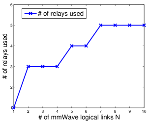
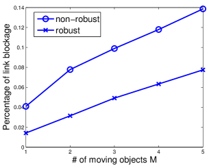
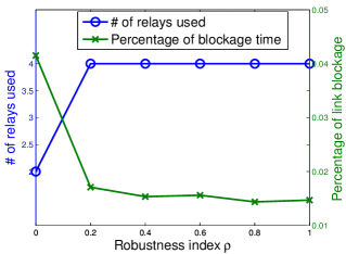
(a) Effect of the number of logical links with $\rho=1$	(b) Effect of the number of moving subjects with $\rho=1$, $N=5$	(c) Effect of the robustness index with $M=1,N=5$

Figure 3: Performance of RMRP in an mmWave home network deployed in a 10m$\times$10m room.

Fig. 3(a) shows the number of relays when relay candidate locations and obstacles are fixed, while the number of mmWave logical links varies. In this set of experiments, all logical links are feasible. More relays are needed as the number of logical links increases. However, the relationship is not always linear due to the absence of LOS paths between TX/RX pairs and the multiplexing of relays.

Fig. 3(b) show the percentage of link blockage per link when human subjects move randomly in the room. The mobility setup is similar to that in Section III-B. Clearly, As the number of human subjects increases, the percentage of link blockage increases as well. However, the robust scheme leads to 50% less blockage.

Next, we evaluate the impact of robustness index $\rho$. In this setup, 1 human subject moves randomly and there are 5 logical links. Figure 3(c) shows the number of relays used and the percentage of link blockage. As expected, as $\rho$ increases, more relays are used and the link blockage reduces.

VI-B RMURP Performance

We now evaluate the performance of the Bisection Search and GBD algorithm on RMURP. The error tolerance of Bisection Search is set to $TOL=1.0$.

Fig. 4 shows the utility achieved using both methods by varying the number of logical links (Fig. 4(a)), the total number of relays (Fig. 4(b)) and the robustness index (Fig. 4(c)). In all cases, GBD achieves higher utility compared to Bisection Search. Reducing the threshold $TOL$ improves the performance of Bisection Search but comes at a higher computation cost.

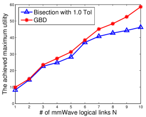
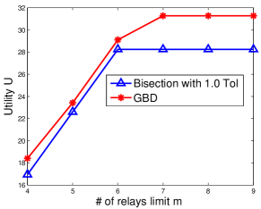
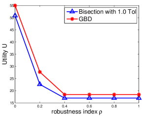
(a) Effect of the number of logical links with $m=7$ and $\rho=1$	(b) Effect of the maximum number of relays with $N=5$ and $\rho=1$	(c) Effect of the robustness index with $m=7$ and $N=5$

Figure 4: Performance of two RMURP solutions in an mmWave home network deployed in a 10m$\times$10m room, Bisection Search algorithm with 1.0 tolerance and GBD algorithm.

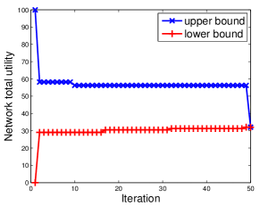
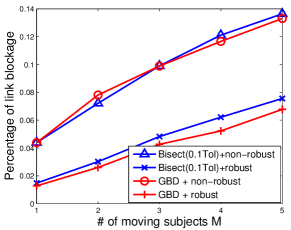
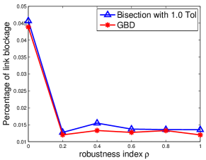
(a) GBD convergence with $N=5$, $m=7$ and $\rho=1$	(b) Effect of the number of moving subjects with $N=5$, $m=7$, and $\rho=1$	(c) Effect of the robustness index with $N=5$, $m=7$, and $M=1$

Figure 5: Performance of RMURP in an mmWave home network deployed in a 10m$\times$10m room.

Fig. 5(a) demonstrates the convergence of the GBD algorithm. As shown in Fig. 5(a), over time, the upper bound (solutions to the master problem) is non-increasing; and the lower bound (solutions to the primary problem) is non-decreasing. The algorithm converges to the optimal solution after 50 iterations when the upper bound equals to the lower bound.

Fig. 5(b)(c) shows the percentage of link blockage per link under RMURP when human subjects move randomly in the room by varying the number of moving subjects and the robustness index, respectively. In both cases, GBD achieves lower percentage of blockage. This implies that the relay selection in GBD has more spatial diversity.

VII Conclusion

In this paper, we formulated two robust relay placement problems in mmWave WPANs, namely, robust minimum relay placement problem (RMRP) and robust maximum utility relay placement (RMURP) for better connectivity and robustness against link blockage. Under the D-norm uncertainty model, RMRP and RMURP were casted as MILP and MINLP problems. Efficient algorithms were devised and evaluated using simulations.

For future work, we will incorporate more complex interference and antenna models in the robustness formulation. Another interesting agenda is to explore the use of passive relays in mmWave WPANs.

References

- [1] C. Anderson and T. Rappaport, “In-building wideband partition loss measurements at 2.5 and 60GHz,” IEEE Transactions on Wireless Communication, vol. 3, no. 3, pp. 922–928, May 2004.
- [2] R. C. Daniels, J. N. Murdock, T. S. Rappaport, and R. W. Heath, “60GHz wireless: Up close and personal,” IEEE Microwave Magazine, vol. 11, no. 7, pp. 44–50, Dec. 2010.
- [3] D. Halperin, S. Kandula, J. Padhye, P. Bahl, and D. Wetherall, “Augmenting data center networks with multi-gigabit wireless links,” in ACM SIGCOMM, Aug. 2011.
- [4] C. Yiu and S. Singh, “Empirical capacity of mmWave WLANs,” IEEE Journal Selected Area in Communications, vol. 27, no. 8, pp. 1479–1487, Oct. 2009.
- [5] S. Singh, R. Mudumbai, and U. Madhow, “Medium access control for 60GHz outdoor mesh networks with highly directional links,” in IEEE INFOCOM, Apr. 2009.
- [6] ——, “Distributed coordination with deaf neighbors: efficient medium access for 60GHz mesh networks,” in IEEE INFOCOM, May 2010.
- [7] S. Singh, F. Ziliotto, U. Madhow, E. M. Belding-Royer, and M. J. W. Rodwell, “Millimeter wave WPAN: Cross-layer modeling and multi-hop architecture,” in IEEE INFOCOM, May. 2007.
- [8] C. Yiu and S. Singh, “Link selection for point-to-point 60GHz networks,” in IEEE ICC, May 2010.
- [9] J. Qiao, L. X. Cai, X. Shen, and J. W. Mark, “Enabling multi-hop concurrent transmissions in 60 ghz wireless personal area networks,” IEEE Transactions on Wireless Communications, vol. 10, no. 11, pp. 3824–3833, Nov. 2011.
- [10] A. Valdes-Garcia, “Millimeter-wave communications using a reflector,” Patent US 2012/0 206 299 A1, 08 16, 2012. [Online]. Available: http://www.google.com/patents/US20120206299.
- [11] K. W. Brown, “Directed energy beam virtual fence,” Patent US 2009/0 256 706 A1, 10 15, 2009. [Online]. Available: http://www.google.com/patents/US20090256706.
- [12] X. Zhou, Z. Zhang, Y. Zhu, Y. Li, S. Kumar, A. Vahdat, B. Y. Zhao, and H. Zheng, “Mirror mirror on the ceiling: Flexible wireless links for data centers,” in ACM SIGCOMM, Aug. 2012.
- [13] K. Yang, J. Huang, Y. Wu, X. Wang, and M. Chiang, “Distributed robust optimization part I: Framework and example,” in Technical Report, Princeton University, Jan. 2009.
- [14] C.-S. Sum, Z. Lan, and etc, “A multi-gbps Millimeter-wave WPAN system based on STDMA with heuristic scheduling,” in IEEE Globecom, Nov. 2009.
- [15] L. X. Cai, L. Cai, X. Shen, and J. W. Mark, “Efficient resource management for mmWave WPANs,” in IEEE WCNC, Mar. 2007.
- [16] ——, “Spatial multiplexing capacity analysis of mmWave WPANs with directional antennae,” in IEEE GLOBECOM, Nov. 2007.
- [17] ——, “Rex: A randomized exclusive region based scheduling scheme for mmWave WPANs with directional antenna,” IEEE Transactions on Wireless Communications, vol. 9, no. 1, pp. 113–121, Jan. 2010.
- [18] S. Singh, F. Ziliotto, U. Madhow, E. M. Belding, and M. Rodwell, “Blockage and directivity in 60 GHz wireless personal area networks: From cross-layer model to multihop mac design,” IEEE Journal Selected in Communications, vol. 19, no. 5, pp. 1513–1527, Oct. 2009.
- [19] M. X. Gong, R. Stacey, D. Akhmetov, and S. Mao, “A directional CSMA/CA protocol for mmWave wireless PANs,” in IEEE WCNC, Apr. 2010.
- [20] M. X. Gong, D. Akhmetov, R. Want, and S. Mao, “Directional CSMA/CA protocol with spatial reuse for mmWave wireless networks,” in IEEE GLOBECOM, Dec. 2010.
- [21] ——, “Multi-user operation in mmWave wireless networks,” in IEEE ICC, Jun. 2011.
- [22] Z. Lan and J. W. etc, “Directional relay with spatial time slot scheduling for mmWave WPAN systems,” in IEEE VTC Spring, May 2010.
- [23] Z. Lan, C. sean Sum, J. Wang, T. Baykas, J. Gao, H. Nakase, H. Harada, and S. Kato, “Deflect routing for throughput improvement in muti-hop millimeter-wave wpan system,” in IEEE WCNC, Apr. 2009.
- [24] P. Dutta, V. Mhatre, D. Panigrahi, and R. Rastogi, “Joint routing and scheduling in multi-hop wireless networks with directional antennas,” in IEEE Infocom, Mar. 2010.
- [25] D. Li, C. Yin, and C. Chen, “A selection region based routing protocol for random mobile ad hoc networks with directional antennas,” in IEEE Globecom, Dec. 2010.
- [26] G. Zheng, C. Hua, K. Vu, R. Zheng, and Q. Wang, “Robust reflector placement in 60GHz mmWave wireless personal area networks,” in IEEE RTAS, Work-in-Progress, Apr. 2012.
- [27] F. Bai and A. Helm, A Survey of Mobility Modeling and Analysis in Wireless Adhoc Networks. Springer, Oct. 2006.
- [28] I. ILOG. CPLEX optimization studio for academics. [Online]. Available: http://www-01.ibm.com/software/websphere/products/optimization /academic-initiative/.
- [29] D. Li and X. Sun, Nonlinear Integer Programming. Springer, 2006.
- [30] C. Hua and R. Zheng, “Robust topology engineering in multiradio multichannel wireless networks,” IEEE Transactions on Mobile Computing, vol. 11, no. 3, pp. 492–503, Mar. 2012.
- [31] T. H. Cormen, Introduction to Algorithms. The MIT Press, Jul. 2009.