Solitary-wave solutions in binary mixtures of Bose-Einstein condensates under periodic boundary conditions

Abstract

We derive solitary-wave solutions within the mean-field approximation in quasi-one-dimensional binary mixtures of Bose-Einstein condensates under periodic boundary conditions, for the case of an effective repulsive interatomic interaction. The particular gray-bright solutions that give the global energy minima are determined. Their characteristics and the associated dispersion relation are derived. In the case of weak coupling, we diagonalize the Hamiltonian analytically to obtain the full excitation spectrum of “quantum” solitary-wave solutions.

I Introduction

The question of solitary-wave solutions in trapped atomic Bose-Einstein condensed gases has received considerable attention in recent years. Remarkably, solitary waves have been created and observed experimentally in both one-component burger ; phillips ; br1 ; br2 and two-component systems becker . The easiest problem that one can consider is that of a quasi-one-dimensional Bose-Einstein condensate which extends to infinity with an effective repulsive interaction. In this case and within the mean-field approximation, the system is described by the nonlinear Schrödinger equation, which supports solitary-wave solutions, as was shown initially by Tsuzuki Tsu , and by Zakharov and Shabat ZS .

If one imposes periodic boundary conditions in a finite period of some fixed length, there are significant differences. It is no longer possible to work in the thermodynamic limit, and it is necessary to impose the particle number normalization condition as well as the constraint of periodicity. This problem has been addressed within the mean-field approximation by Carr et al. carr , for static solutions and by the authors of this study for the more general case of moving solutions SMKJ . These were shown to be Jacobi elliptic functions. The excitation spectrum of the many-body problem of a single-component Bose gas interacting via a contact potential has also been studied by Lieb lieb . This study assumed periodic boundary conditions and also considered the limit of an infinite period $L_{0}$ and an infinite number of particles $N$ with $N/L_{0}$ constant. The excitation spectrum was found to consist of two branches, one of which was later identified as corresponding to solitary-wave excitation id .

The problem of solitary-wave solutions in binary mixtures of Bose-Einstein condensates has also been studied theoretically by many people, see, e.g., trillo ; christo ; shalaby ; santos ; anglin ; kevrekidis ; berloff ; konotop ; liu . In the case of strictly one-dimensional motion with the two condensates extending over an infinite line, the coupled system of two non-linear Schrödinger equations that describe the two order parameters (within the mean-field approximation) has been studied in the context of integrable systems by Manakov manakov .

In the present study we present mean-field solitary-wave solutions for a two-component Bose-Einstein condensate with repulsive interatomic interactions for a periodic system of finite length $L_{0}$. To determine these solutions we impose constraints on the particle number for each component as well as the constraint of periodicity for each species. This formidable set of constraints is necessary to determine the solution and the dispersion relation, i.e., the energy versus the angular momentum, of this system.

As in the case of a single component, the solitary-wave solutions are again found to be Jacobi elliptic functions kavoulakis1 . In this case, however, the presence of the second component permits several qualitatively different solutions, i.e., “gray-gray” and “gray-bright” solitons. We will argue that the gray-bright solution has the lowest energy for particular choices of the phase winding numbers and for interactions which are weak in comparison with the kinetic energy of the atoms. The numerical solution of the equations which result from these constraints also suggests that the choice of the winding numbers does not change for moderate couplings.

This problem is also intimately connected with the “yrast” problem, i.e., with the evaluation of the state of lowest energy with some fixed angular momentum. The yrast state was determined in Refs. kavoulakis1 ; kavoulakis2 and coincides Ueda ; equiv with the gray-bright solution found below. The connection with the results of Refs. kavoulakis1 ; kavoulakis2 , obtained directly by minimization of the energy at fixed angular momentum, is clarified and gives further support to the belief that the yrast states are indeed the gray-bright solutions. Although gray-gray solutions are also possible, the gray-bright solution has a lower energy. The qualitative explanation of this result is simple. The density depression found in the gray component is (at least partially) filled by the bright component. This leads to a more uniform total density and thus to a lower energy provided that the interatomic interaction is repulsive.

Finally, in the particular case of weak interatomic interactions, the complete energy spectrum of the system is determined by diagonalization the many-body Hamiltonian. This is done by identifying certain bilinears of the annihilation and creation operators with angular momentum operators. Under the assumption of weak coupling, the interaction terms in the Hamiltonian can be re-expressed in terms of Casimir operators and thus permit the analytic diagonaliztion of the Hamiltonian.

In the following we first present our model in Sec. II and adopt an ansatz that allows us to solve the two coupled nonlinear Gross-Pitaevskii equations. In Sec. III we evaluate the energy and the angular momentum of these solutions. In Sec. IV we impose the constraints that are set by particle normalization and periodicity. In Sec. V we consider the nature of these solutions in the limit of weak interactions, and in Sec. VI we present numerical results for our solutions for stronger coupling. In Sec. VII we present the results from diagonalization of the many-body Hamiltonian. Conclusions and an overview are given in Sec. VIII.

II Model and solitary-wave solutions

Within the mean-field approximation, the order parameters of the two distinguishable species (labelled as $A$ and $B$) satisfy the coupled system of the following integrable non-linear equations (Manakov system),

$$i\frac{\partial\psi_{A}}{\partial t} = -\frac{1}{2}\psi_{A}^{\prime\prime}+(\gamma_{AA}|\psi_{A}|^{2}+\gamma_{AB}|\psi_{B}|^{2})\psi_{A}$$ (1)

$$i\frac{\partial\psi_{B}}{\partial t} = -\frac{1}{2}\psi_{B}^{\prime\prime}+(\gamma_{BA}|\psi_{A}|^{2}+\gamma_{BB}|\psi_{B}|^{2})\psi_{B},$$ (2)

where $\hbar=1$ and the masses of the two species are assumed to be equal (and are also set to unity). In addition $\gamma_{ij}$ is the matrix element for collisions between species $i$ and $j$.

The solitary-wave solutions have the form of traveling waves with the particle density of each species moving with a constant velocity, $u$,

$$\psi_{A}=\sqrt{n_{A}(z)}e^{i\Phi_{A}(z)}e^{-i\mu_{A}t}$$ (3)

$$\psi_{B}=\sqrt{n_{B}(z)}e^{i\Phi_{B}(z)}e^{-i\mu_{B}t},$$ (4)

where $z=x-ut$, $n_{A}$ and $n_{B}$ are the particle densities, and $\mu_{A}$ and $\mu_{B}$ are the chemical potentials of the two species. Here $x$ is the spatial variable which is assumed to be periodic on the interval $0\leq x\leq L_{0}$. Following standard procedures, we separate the real and imaginary parts of these equations to find that

$$\Phi_{A,B}^{\prime}=u+\frac{C_{A,B}}{n_{A,B}},$$ (5)

where $C_{A}$ and $C_{B}$ are constants of integration, and also

$$\frac{1}{2}(\sqrt{n_{A}})^{\prime\prime}=-\frac{1}{2}u^{2}\sqrt{n_{A}}+\frac{1}{2}\frac{C_{A}^{2}}{n_{A}^{3/2}}$$

$$+(\gamma_{AA}n_{A}+\gamma_{AB}n_{B}-\mu_{A})\sqrt{n_{A}}$$

(6)

$$\frac{1}{2}(\sqrt{n_{B}})^{\prime\prime}=-\frac{1}{2}u^{2}\sqrt{n_{B}}+\frac{1}{2}\frac{C_{B}^{2}}{n_{B}^{3/2}}$$

$$+(\gamma_{BA}n_{A}+\gamma_{BB}n_{B}-\mu_{B})\sqrt{n_{B}}.$$

(7)

Making the ansatz

$$n_{B}=\kappa n_{A}+\lambda,$$ (8)

where $\kappa$ and $\lambda$ are parameters independent of the space and time variables, we can integrate these equations. With this ansatz, the left side of Eqs. (6) and (7) become functions of $n_{A}$ and $n_{B}$ respectively that can be integrated to yield

$$\frac{1}{4}n_{A}^{\prime 2}=(\gamma_{AA}+\kappa\gamma_{AB})n_{A}^{3}\hskip 60.00009pt$$

$$-2(\frac{1}{2}u^{2}+\mu_{A}-\lambda\gamma_{AB})n_{A}^{2}+E_{A}n_{A}-C_{A}^{2}$$ (9)

$$\frac{1}{4}n_{B}^{\prime 2}=(\frac{\gamma_{BA}}{\kappa}+\gamma_{BB})n_{B}^{3}\hskip 60.00009pt$$

$$-2(\frac{1}{2}u^{2}+\mu_{B}+\frac{\lambda}{\kappa}\gamma_{BA})n_{B}^{2}+E_{B}n_{B}-C_{B}^{2},$$ (10)

where $E_{A}$ and $E_{B}$ are integration constants. Consistency of the ansatz translates into three equations that relate the integration constants and the chemical potentials of the two species together with the condition arising from the identification of the coefficients of $n_{A}^{3}$

$$\gamma_{AA}+\kappa\gamma_{AB}=\gamma_{AB}+\kappa\gamma_{BB}\equiv\gamma.$$ (11)

Our ansatz constrains the integration constants, thus restricting the full solution space of our system of equations. In the generic case there are six integration constants in Eqs. (9) and (10), namely $E_{A},E_{B},\mu_{A},\mu_{B},C_{A}$ and $C_{B}$ as well as the two constants $\kappa$ and $\lambda$ arising from the ansatz. There are also four consistency conditions which reduces the number of free constants to four for any given propagation velocity, $u$. The integration constant arising from the integration of Eqs. (9) and (10) is not included in this counting since it merely corresponds to a translation of the solution. However, the solution must also satisfy five constraints, namely two constraints of particle-number normalization, two phase-matching constraints, and one constraint which sets the period of the solution to $L_{0}$. In short, there are too many constraints.

One possible way out of this dilemma would be to view the velocity of propagation, $u$, as a parameter to be set by the constraints. This, however, would lead to the unphysical result that the velocity of the waves cannot be changed without altering the properties of the atoms involved. If we ignore the ansatz, $u$ is expected to be a free parameter, since we have a total of six integration constants (including the chemical potentials) and six constraints (i.e., two particle number normalizations, two phase matchings and two density matchings.) The restriction on $u$ must be viewed as an artifact of the ansatz.

A more satisfactory way to deal with this problem is to fine tune the coupling constants. If the masses of the two components are equal, it follows that $\gamma_{AB}$ and $\gamma_{BA}$ are trivially equal. If, however, $\gamma_{AA}=\gamma_{AB}=\gamma_{BB}\equiv\gamma_{0}$ (i.e., if the scattering lengths between the same and the different species are all equal), then the condition of Eq. (11) becomes trivial, and we have five free constants and five constraints. This allows the velocity of propagation to be a free parameter. We thus proceed under the assumption that all the coupling constants are equal. Note that in this case Eq. (11) implies that $\gamma=\gamma_{0}(1+\kappa)$.

It is convenient to factorize the right sides of Eqs. (9) and (10) to obtain the equations

$$\frac{1}{2}n_{A}^{\prime 2}=2\gamma(n_{A}-\rho_{A1})(n_{A}-\rho_{A2})(n_{A}-\rho_{A3})$$ (12)

$$\frac{1}{2}n_{B}^{\prime 2}=\frac{2\gamma}{\kappa}(n_{B}-\rho_{B1})(n_{B}-\rho_{B2})(n_{B}-\rho_{B3}),$$ (13)

where the roots in these equations are written in ascending order. Compatibility between Eqs. (9) and (10) and Eqs. (12), and (13) requires that

$$C_{A}^{2} = \gamma\rho_{A1}\rho_{A2}\rho_{A3}$$ (14)

$$C_{B}^{2} = \frac{\gamma}{\kappa}\rho_{B1}\rho_{B2}\rho_{B3}.$$ (15)

Since both densities have maximum and minimum values where their derivatives must vanish, all roots must be real. Because of the positivity of $n_{A}^{\prime 2}$, the solution of Eq. (12) is trapped between $\rho_{A1}=n_{A,{\rm min}}$ and $\rho_{A2}=n_{A,\rm{max}}$, i.e., between the minimum and the maximum densities of species $A$. There are two possibilities for Eq. (13). For one of these, $\kappa>0$, $\rho_{B1}=n_{B,{\rm min}}$, and $\rho_{B2}=n_{B,{\rm max}}$. For the other, $\kappa<0$, $\rho_{B2}=n_{B,{\rm min}}$, and $\rho_{B3}=n_{B,{\rm max}}$. The first case corresponds to a gray-gray solution; the second corresponds to a gray-bright solution.

For the gray-gray solution, we note that Eq. (13) reduces to Eq. (12) if

$$n_{B,{\rm min}} = \kappa n_{A,{\rm min}}+\lambda$$ (16)

$$n_{B,{\rm max}} = \kappa n_{A,{\rm max}}+\lambda$$ (17)

$$\rho_{B3} = \kappa\rho_{A3}+\lambda.$$ (18)

The solution of Eqs. (12), and (13) can then be expressed in terms of Jacobi elliptic functions as

$$n_{A}=n_{A,{\rm min}}+(n_{A,{\rm max}}-n_{A,{\rm min}}){\rm sn}^{2}(\frac{2K(m)z}{L_{0}}|m)$$ (19)

$$n_{B}=n_{B,{\rm min}}+(n_{B,{\rm max}}-n_{B,{\rm min}}){\rm sn}^{2}(\frac{2K(m)z}{L_{0}}|m),$$ (20)

where

$$m=\frac{n_{A,{\rm max}}-n_{A,{\rm min}}}{\rho_{A3}-n_{A,{\rm min}}}=\frac{n_{B,{\rm max}}-n_{B,{\rm min}}}{\rho_{B3}-n_{B,{\rm min}}},$$ (21)

and where the first elliptic integral $K(m)$ satisfies the periodicity constraint

$$K(m)=\frac{L_{0}}{\sqrt{8m}}\sqrt{2\gamma(n_{A,{\rm max}}-n_{A,{\rm min}})}.$$ (22)

Equation (18) implies that $m$ is the same in Eqs. (19) and (20). In this general form, the five independent constants in the solution space are $n_{A,{\rm max}},n_{A,{\rm min}},\kappa,\lambda$, and $m$.

In the gray-bright case ($\kappa<0$), the reduction of Eq. (13) to Eq. (12) requires that

$$n_{B,{\rm min}} = \kappa n_{A,{\rm max}}+\lambda$$ (23)

$$n_{B,{\rm max}} = \kappa n_{A,{\rm min}}+\lambda$$ (24)

$$\rho_{B1} = \kappa\rho_{A3}+\lambda.$$ (25)

The solution of Eqs. (12) and (13) is now

$$n_{A}=n_{A,{\rm min}}+(n_{A,{\rm max}}-n_{A,{\rm min}}){\rm sn}^{2}(\frac{2K(m)z}{L_{0}}|m)$$ (26)

$$n_{B}=n_{B,{\rm min}}+(n_{B,{\rm max}}-n_{B,{\rm min}}){\rm cn}^{2}(\frac{2K(m)z}{L_{0}}|m),$$ (27)

where

$$m=\frac{n_{A,{\rm max}}-n_{A,{\rm min}}}{\rho_{A3}-n_{A,{\rm min}}}=\frac{n_{B,{\rm max}}-n_{B,{\rm min}}}{n_{B,{\rm max}}-\rho_{B1}},$$ (28)

and $K(m)$ satisfies the periodicity constraint given above. Again, the five independent constants in the solution space are $n_{A,{\rm max}},n_{A,{\rm min}},\kappa,\lambda$, and $m$.

For both the gray-gray and the gray-bright cases, we note that Eqs. (12) and (13) have an interesting limiting form when $\kappa\to-1$ and $\rho_{A3}\to+\infty$ in such a way that $(1+\kappa)\rho_{A3}$ is finite. The fact that $\rho_{A3}\to+\infty$ tells us that $m\to 0$. Hence, the elliptic functions ${\rm sn}(2K(m)z/L_{0}|m)$, and ${\rm cn}(2K(m)z/L_{0}|m)$ become the regular trigonometric functions $\sin(\pi z/L_{0})$ and $\cos(\pi z/L_{0})$, respectively. The periodicity condition of Eq. (22) assumes the form

$$\lim_{\kappa\to-1}\frac{m}{1+\kappa}=\frac{L_{0}^{2}}{\pi^{2}}\gamma_{0}(n_{A,{\rm max}}-n_{A,{\rm min}}).$$ (29)

The gray-gray solution then simplifies to

$$n_{A}=n_{A,{\rm min}}+(n_{A,{\rm max}}-n_{A,{\rm min}})\sin^{2}(\frac{\pi z}{L_{0}})$$ (30)

$$n_{B}=n_{B,{\rm min}}+(n_{B,{\rm max}}-n_{B,{\rm min}})\sin^{2}(\frac{\pi z}{L_{0}}),$$ (31)

and the gray-bright solution becomes

$$n_{A}=n_{A,{\rm min}}+(n_{A,{\rm max}}-n_{A,{\rm min}})\sin^{2}(\frac{\pi z}{L_{0}})$$ (32)

$$n_{B}=n_{B,{\rm min}}+(n_{B,{\rm max}}-n_{B,{\rm min}})\cos^{2}(\frac{\pi z}{L_{0}}).$$ (33)

Since the total density is more uniform in gray-bright case and since the interaction is repulsive, this solution will have a lower energy. The remainder of this paper will focus on the analysis of this solution only.

III Dispersion relation: energy versus angular momentum

In this section we evaluate the energy and the angular momentum of the system in the gray-bright case. We begin with the angular momentum, which has the form

$$L = \frac{L_{0}}{2\pi}\int\psi_{A}^{*}(-i\frac{d}{dx})\psi_{A}dx+\frac{L_{0}}{2\pi}\int\psi_{B}^{*}(-i\frac{d}{dx})\psi_{B}dx$$ (34)

$$= \frac{L_{0}}{2\pi}\int(n_{A}\Phi_{A}^{\prime}+n_{B}\Phi_{B}^{\prime})dx.$$

We can eliminate $\Phi_{A}^{\prime}$ and $\Phi_{B}^{\prime}$ using the equations for the conservation of particles, Eqs. (5), to obtain

$$\frac{2\pi}{L_{0}}L=u(N_{A}+N_{B})+(C_{A}+C_{B})L_{0},$$ (35)

where $N_{A}$ and $N_{B}$ are the particle numbers for the two species.

The energy is given by

$$E=\int\{\frac{1}{2}|\psi_{A}^{\prime}|^{2}+\frac{1}{2}|\psi_{B}^{\prime}|^{2}+\frac{1}{2}\gamma_{0}(|\psi_{A}|^{2}+|\psi_{B}|^{2})^{2}\}dx,$$ (36)

which can also be written as

$$E=\int\frac{1}{2}\{\frac{(n_{A}^{\prime})^{2}}{4n_{A}}+n_{A}(u+\frac{C_{A}}{n_{A}})^{2}+\frac{(n_{B}^{\prime})^{2}}{4n_{B}}$$

$$+n_{B}(u+\frac{C_{B}}{n_{B}})^{2}+\gamma_{0}(n_{A}+n_{B})^{2}\}dx.$$ (37)

Using Eqs. (12)–(15) together with the particle number normalization, $E$ can be expressed in the form

$$E-E_{0}=\frac{1}{2}u^{2}(N_{A}+N_{B})+u(C_{A}+C_{B})L_{0}$$

$$-\frac{\gamma}{2}((2-\frac{1}{m})n_{A,{\rm min}}+(1+\frac{1}{m})n_{A,{\rm max}})N_{A}$$

$$-\frac{\gamma}{2\kappa}((2-\frac{1}{m})n_{B,{\rm max}}+(1+\frac{1}{m})n_{B,{\rm min}})N_{B}$$

$$+\frac{\gamma}{2}(2n_{A,{\rm max}}n_{A,{\rm min}}+\frac{1}{m}n_{A,{\rm max}}^{2}+(1-\frac{1}{m})n_{A,{\rm min}}^{2})L_{0}$$

$$+\frac{\gamma}{2\kappa}(2n_{B,{\rm max}}n_{B,{\rm min}}+\frac{1}{m}n_{B,{\rm min}}^{2}+(1-\frac{1}{m})n_{B,{\rm max}}^{2})L_{0},$$

(38)

where

$$E_{0}=\int_{-L_{0}/2}^{L_{0}/2}[\frac{\gamma}{2}n_{A}^{2}+\frac{\gamma}{2\kappa}n_{B}^{2}+\frac{\gamma_{0}}{2}(n_{A}+n_{B})^{2}].$$ (39)

It is possible to derive a simple form for $E_{0}$ using the normalization constraints (see Appendix 2). In this way we get

$$E_{0}=\gamma_{0}(1+\kappa)^{2}\Big{[}n_{A,{\rm min}}(2N_{A}-n_{A,{\rm min}}L_{0}$$

$$-\frac{2(m+1)}{3m}\Delta n_{A}L_{0})+\frac{2(m+1)}{3m}N_{A}\Delta n_{A}-\frac{1}{3m}\Delta n_{A}^{2}L_{0}\Big{]}$$

$$+\gamma_{0}\Big{[}\frac{N_{A}N_{B}}{L_{0}}-\frac{3}{2}\kappa\frac{N_{A}^{2}}{L_{0}}-\kappa^{2}\frac{N_{A}^{2}}{L_{0}}+\frac{N_{B}^{2}}{L_{0}}+\frac{1}{2\kappa}\frac{N_{B}^{2}}{L_{0}}\Big{]}.$$

(40)

In the limiting case $\kappa\to-1$ with $(1+\kappa)=O(m)$, $E_{0}\to\gamma_{0}(N_{A}+N_{B})^{2}/(2L_{0})$, which is indeed the interaction energy of a gas of constant density with $N_{A}+N_{B}$ particles. In this limit, the remaining energy is

$$E-E_{0}\rightarrow\frac{1}{2}u^{2}N+u(C_{A}+C_{B})L_{0}+\frac{1}{2}\frac{\pi^{2}}{L_{0}^{2}}N.$$ (41)

Here, we have used the limiting form of the periodicity condition, Eq. (29), to eliminate quotients of the form $(1+\kappa)/m$. If the winding number $q_{A}=0$ or $q_{B}=0$, then $m=0$ and the velocity becomes $u=\pi/L_{0}$, as it should. Since we also have Eq. (35), it is possible to write

$$E-E_{0}\rightarrow\frac{2\pi^{2}}{L_{0}^{2}}L=\frac{u}{(L_{0}/2\pi)}L.$$ (42)

This is consistent with the equation $\partial E/\partial L=\Omega$, where $\Omega$ is the angular velocity of the condensate.

IV Constraints

The particle number normalization constraints tell us that

$$\int_{-L_{0}/2}^{L_{0}/2}n_{A,B}dz=N_{A,B}.$$ (43)

Using the integrals given in Appendix 2, these equations become

$$n_{A,{\rm min}}L_{0}+(n_{A,{\rm max}}-n_{A,{\rm min}})\frac{L_{0}}{m}(1-\frac{E(m)}{K(m)})$$

$$=N_{A}$$ (44)

$$n_{B,{\rm min}}L_{0}+(n_{B,{\rm max}}-n_{B,{\rm min}})\frac{L_{0}}{m}(m-1+\frac{E(m)}{K(m)})$$

$$=N_{B},$$ (45)

where $K(m)$ and $E(m)$ are the usual elliptic integrals.

The phase matching constraints,

$$\int_{-L_{0}/2}^{-L_{0}/2}\Phi_{A,B}^{\prime}dz=2\pi q_{A,B},$$ (46)

imply that

$$uL_{0}+C_{A,B}\int_{-L_{0}/2}^{-L_{0}/2}\frac{1}{n_{A,B}}dz=2\pi q_{A,B}.$$ (47)

Here $q_{A}$ and $q_{B}$ are the winding numbers of the two species. Equations (14) and (15) allow us to determine $C_{A}$ and $C_{B}$ as

$$C_{A}^{2}=\gamma n_{A,{\rm min}}n_{A,{\rm max}}[n_{A,{\rm min}}+\frac{n_{A,{\rm max}}-n_{A,{\rm min}}}{m}]$$ (48)

$$C_{B}^{2}=\frac{\gamma}{\kappa}n_{B,{\rm min}}n_{B,{\rm max}}[n_{B,{\rm max}}-\frac{n_{B,{\rm max}}-n_{B,{\rm min}}}{m}].$$ (49)

Carrying out the integrations in Eq. (47) and solving for the velocity $u$, we find that

$$u=\frac{2\pi q_{A}}{L_{0}}\pm\sqrt{\frac{n_{A,{\rm max}}}{n_{A,{\rm min}}}}\frac{1}{K(m)}\Pi(1-\frac{n_{A,{\rm max}}}{n_{A,{\rm min}}}|m)$$

$$\times\sqrt{\gamma[n_{A,{\rm min}}+(n_{A,{\rm max}}-n_{A,{\rm min}})/{m}]}$$

(50)

$$u=\frac{2\pi q_{B}}{L_{0}}\pm\sqrt{\frac{n_{B,{\rm min}}}{n_{B,{\rm max}}}}\frac{1}{K(m)}\Pi(1-\frac{n_{B,{\rm min}}}{n_{B,{\rm max}}}|m)$$

$$\times\sqrt{(\gamma/\kappa)[n_{B,{\rm max}}-(n_{B,{\rm max}}-n_{B,{\rm min}})/{m}]},$$ (51)

where $\Pi(a|m)$ is the third elliptic integral. Note that the sign ambiguity that appears in Eqs. (50) and (51) comes from the ambiguity in the sign of the constants $C_{A},C_{B}$. Equations (9) and (10) for the densities $n_{A}$ and $n_{B}$ involve only $C_{A,B}^{2}$, hence there is an ambiguity in the signs of $C_{A,B}$ in the solutions. The only place where these signs are important are in the phase matching constraints, where the winding numbers also appear. Therefore, a solution of the phase matching constraints involves not only a choice of the winding numbers $q_{A}$ and $q_{B}$, but also a choice for the signs of $C_{A,B}$. The final constraint is the periodicity constraint, Eq. (22), encountered earlier. These five constraints are sufficient to determine the solution.

V Weak-coupling limit

In the particular case $m\to 0$ the periodicity constraint of Eq. (22) has, to lowest order, a particularly simple form (see Appendix 1):

$$\frac{1+\kappa}{m}=\frac{\pi^{2}(1+m/2)}{L_{0}^{2}\gamma_{0}(n_{A,{\rm max}}-n_{A,{\rm min}})}+{\cal O}(m^{2}).$$ (52)

Since in general it is not necessarily true that $\Delta n_{A}\equiv n_{A,{\rm max}}-n_{A,{\rm min}}\ll 1/L_{0}$, from the above equation follows that we should also take the limit $\kappa\to-1$, so that the value of $\lim_{(\kappa,m)\to(-1,0)}(1+\kappa)/{m}$ is finite and determines $\Delta n_{A}$.

In this limit, the normalization constraints of Eqs. (44) and (45) can be written as

$$\frac{n_{A,{\rm max}}+n_{A,{\rm min}}}{2}+\frac{\Delta n_{A}}{16}m+{\cal O}(m^{2})=\frac{N_{A}}{L_{0}}$$ (53)

$$\frac{n_{B,{\rm max}}+n_{B,{\rm min}}}{2}-\frac{\Delta n_{B}}{16}m+{\cal O}(m^{2})=\frac{N_{B}}{L_{0}}.$$ (54)

Setting $\bar{n}_{A,B}\equiv(n_{A,B,{\rm max}}+n_{A,B,{\rm min}})/{2}$, we see that $\bar{n}_{A,B}=N_{A,B}/{L_{0}}$ to lowest order in $m$.

The phase constants $C_{A}$ and $C_{B}$ are given as

$$C_{A} = \pm\frac{\pi}{L_{0}}\sqrt{n_{A,{\rm max}}n_{A,{\rm min}}}\sqrt{1+m\frac{\bar{n}_{A}}{\Delta n_{A}}}$$ (55)

$$= \pm\frac{\pi}{L_{0}}\sqrt{n_{A,{\rm max}}n_{A,{\rm min}}}(1+\frac{1}{2}m\frac{\bar{n}_{A}}{\Delta n_{A}})$$

$$C_{B} = \pm\frac{\pi}{L_{0}}\sqrt{n_{B,{\rm max}}n_{B,{\rm min}}}\sqrt{1-m\frac{\bar{n}_{B}}{\Delta n_{B}}}$$ (56)

$$= \pm\frac{\pi}{L_{0}}\sqrt{n_{B,{\rm max}}n_{B,{\rm min}}}(1-\frac{1}{2}m\frac{\bar{n}_{B}}{\Delta n_{B}}).$$

Using the asymptotic expansion of $\Pi(a|m)$ and $K(m)$ (see Appendix 1), we see that the phase constraints of Eqs. (50) and (51) can be written as

$$u = \frac{\pi}{L_{0}}(2q_{A}\mp 1\mp\frac{m}{2}\frac{\sqrt{n_{A,{\rm max}}n_{A,{\rm min}}}}{\Delta n_{A}})+{\cal O}(m^{2})$$ (57)

$$u = \frac{\pi}{L_{0}}(2q_{B}\mp 1\pm\frac{m}{2}\frac{\sqrt{n_{B,{\rm max}}n_{B,{\rm min}}}}{\Delta n_{B}})+{\cal O}(m^{2}).$$ (58)

Here, the signs that appear in the above formulae are to be determined by the signs of the phase constants $C_{A}$ and $C_{B}$ (positive, upper sign; negative lower sign), which still need to be determined. We also note that these expansion formulae are valid only if $\Delta n_{A,B}/{\bar{n}}_{A,B}\gg m$ since the expansions of Eqs. (55) and (56) are not otherwise valid.

It is also possible to expand the particle densities near $m=0$ by making use of the Lambert series of the Jacobi elliptic functions (see Appendix 1). This gives us

$$n_{A}(z)=n_{A,{\rm min}}+\Delta n_{A}[(\frac{1}{2}-\frac{1}{2}\cos(\frac{2\pi z}{L_{0}}))$$

$$+\frac{m}{16}(1-\cos(\frac{4\pi z}{L_{0}}))]+O(m^{2})$$ (59)

$$n_{B}(z)=n_{B,{\rm min}}+\Delta n_{B}[(\frac{1}{2}+\frac{1}{2}\cos(\frac{2\pi z}{L_{0}}))$$

$$-\frac{m}{16}(1-\cos(\frac{4\pi z}{L_{0}}))]+O(m^{2}).$$ (60)

The angular momentum given by Eq. (35) has the expanded form

$$\frac{2\pi}{L_{0}}L=u(N_{A}+N_{B})\pm\pi\sqrt{n_{A,{\rm max}}n_{A,{\rm min}}}(1+\frac{1}{2}m\frac{\bar{n}_{A}}{\Delta n_{A}})$$

$$\pm\pi\sqrt{n_{B,{\rm max}}n_{B,{\rm min}}}(1-\frac{1}{2}m\frac{\bar{n}_{B}}{\Delta n_{B}}),$$ (61)

where it is again necessary to assume that $\Delta n_{A,B}\gg m$.

Let us consider now the specific branch $(q_{A},q_{B})=(0,0)$. If the velocity $u>0$, then Eq. (47) demands that $C_{A}<0$ and $C_{B}<0$; hence the lower signs in Eqs. (57) and (58) apply. The only way to realize this while still having a common velocity for the two species is to have $m=0$ exactly. This gives a propagation velocity of $u={\pi(2q_{A}+1)}/{L_{0}}={\pi}/{L_{0}}$. This means that the densities have the form

$$n_{A}(z) = n_{A,{\rm min}}+\Delta n_{A}(\frac{1}{2}-\frac{1}{2}\cos(\frac{2\pi z}{L_{0}}))$$ (62)

$$n_{B}(z) = n_{B,{\rm min}}+\Delta n_{B}(\frac{1}{2}+\frac{1}{2}\cos(\frac{2\pi z}{L_{0}})).$$ (63)

In this case the angular momentum is

$$\frac{2\pi}{L_{0}}L=\frac{\pi}{L_{0}}(N_{A}+N_{B})-\pi\sqrt{n_{A,{\rm max}}n_{A,{\rm min}}}-$$

$$\pi\sqrt{n_{B,{\rm max}}n_{B,{\rm min}}}.$$ (64)

Recalling that $n_{A,{\rm max}}=-n_{B,{\rm min}}+N/L_{0}$ and that $n_{A,{\rm min}}=-n_{B,{\rm max}}+N/L_{0}$, it is easy to show that the maximum value of the angular momentum in this branch is

$$\frac{L_{\rm max}}{N}\equiv\ell_{\rm max}=\frac{1}{2}-\frac{1}{2}\sqrt{x_{A}-x_{B}}.$$ (65)

Making use of the fact that $(n_{B,{\rm min}}+n_{B,{\rm max}})/2=N_{B}/L_{0}+O(m\Delta n_{B})$ we note that this maximum is attained when $n_{B,{\rm min}}n_{B,{\rm max}}$ vanishes and this is only possible when $n_{B,{\rm min}}=0$. Here, we have written the total particle number as $N=N_{A}+N_{B}$, the angular momentum per particle as $\ell=L/N$, and the particle fractions as $x_{A,B}=N_{A,B}/N$. As mentioned earlier, the yrast state of a two-component Bose-Einstein condensate confined in a ring trap was evaluated in Ref. kavoulakis2 . Based on rather general arguments Ueda ; equiv , the present calculation is expected to be equivalent to that of the yrast state. Indeed, the branch found above corresponds to a portion of the first linear branch in the dispersion relation determined in Ref. kavoulakis2 (i.e., for $\ell<x_{B}$). The lowest-energy state obtained in Ref. kavoulakis2 was found to be

$$\Psi_{A} = \sqrt{\frac{N_{A}}{L_{0}}}(c_{0}+c_{1}e^{2\pi iz/L_{0}})$$

$$\Psi_{B} = \sqrt{\frac{N_{B}}{L_{0}}}(d_{0}+d_{1}e^{2\pi iz/L_{0}}),$$ (66)

where

$$|c_{0}|^{2}=\frac{(x_{A}-\ell)(1-\ell)}{x_{A}(1-2\ell)}, |c_{1}|^{2}=\frac{\ell(x_{B}-\ell)}{x_{A}(1-2\ell)}$$

$$|d_{0}|^{2}=\frac{(x_{B}-\ell)(1-\ell)}{x_{B}(1-2\ell)}, |d_{1}|^{2}=\frac{\ell(x_{A}-\ell)}{x_{B}(1-2\ell)}$$ (67)

for this branch. This gives rise to the following densities for the two species

$$n_{A} = \frac{N_{A}}{L_{0}}+\frac{N_{A}}{L_{0}}\left(c_{0}c_{1}^{*}e^{-2\pi iz/L_{0}}+c_{0}^{*}c_{1}e^{2\pi iz/L_{0}}\right)$$

$$n_{B} = \frac{N_{B}}{L_{0}}+\frac{N_{B}}{L_{0}}\left(d_{0}d_{1}^{*}e^{-2\pi iz/L_{0}}+d_{0}^{*}d_{1}e^{2\pi iz/L_{0}}\right).$$ (68)

These become identical to the densities given by Eqs. (62) and (63) if we set

$$c_{0}c_{1}^{*}=-\frac{n_{A,{\rm max}}-n_{A,{\rm min}}}{4N_{A}/L_{0}},d_{0}d_{1}^{*}=\frac{n_{B,{\rm max}}-n_{B,{\rm min}}}{4N_{B}/L_{0}}.$$ (69)

This is compatible with the amplitudes of Eqs. (67).

We consider now the branch $(q_{A},q_{B})=(0,1)$. It will be assumed that the particle wave functions switch continuously to this branch as the angular momentum of the system increases. When applied to the phase matching constraints of Eqs. (47), this continuity demands that $C_{A}<0$ and $C_{B}>0$. To ${\cal O}(m)$ the phase matching condition can be satisfied in two ways. One is by having $m=0$, in which case the densities are exactly as in the $(q_{A},q_{B})=(0,0)$ case. However, the constant $C_{B}$ now changes sign and becomes positive. This means that the angular momentum is given as

$$\frac{2\pi}{L_{0}}L=\frac{\pi}{L_{0}}(N_{A}+N_{B})-\pi\sqrt{n_{A,{\rm max}}n_{A,{\rm min}}}$$

$$+\pi\sqrt{n_{B,{\rm max}}n_{B,{\rm min}}}.$$ (70)

This satisfies the inequality

$$\frac{1}{2}-\frac{1}{2}\sqrt{x_{A}-x_{B}}\leq\ell\leq x_{B}.$$ (71)

This branch corresponds to the remainder of the first linear branch in the dispersion relation of Ref. kavoulakis2 .

The second way is by having

$$\frac{\sqrt{n_{A,{\rm max}}n_{A,{\rm min}}}}{\Delta n_{A}}=\frac{\sqrt{n_{B,{\rm max}}n_{B,{\rm min}}}}{\Delta n_{B}}$$ (72)

to ${\cal O}(1)$. This relation together with the ansatz relations Eqs. (23) and (24) and the normalization conditions Eqs. (53) and (54) to lowest order tell us that $\kappa=-{N_{B}}/{N_{A}}$ and $\lambda={2N_{B}}/{L_{0}}$. This is to be understood as a weak-coupling branch: The periodicity condition of Eq. (52) demands that $\Delta n_{A}={\cal O}(m)$, and this violates the condition $\Delta n_{A,B}/{\bar{n}}_{A,B}\gg m$, unless $\gamma_{0}\ll{1}/{L_{0}}$ is small. The angular momentum has the form

$$L=\frac{N_{A}+N_{B}}{2}-\frac{1}{2}\frac{\sqrt{n_{A,{\rm max}}n_{A,{\rm min}}}}{N_{A}/L_{0}}(N_{A}-N_{B}).$$ (73)

Dividing by the total number of particles $N$, the above equation gives

$$\frac{\sqrt{n_{A,{\rm max}}n_{A,{\rm min}}}}{N_{A}/L_{0}}=\frac{1-2\ell}{x_{A}-x_{B}},$$ (74)

and the propagation velocity becomes

$$u=\frac{\pi}{L_{0}}+\frac{\gamma_{0}N}{2\pi}(1-2\ell).$$ (75)

The minimum and the maximum values of the above angular momentum are given by the inequality

$$x_{B}\leq\ell\leq\frac{1}{2}.$$ (76)

This branch can be identified as the first half of the curved part of the dispersion relation derived in Ref. kavoulakis2 . Note that at $\ell=1/2$ we get $u=\pi/L_{0}$, which is the velocity when $m$ is exactly zero.

The next branch which appears as the angular momentum increases is given by $(q_{A},q_{B})=(1,0)$. Here we have $C_{A}>0$ and $C_{B}<0$. To order ${\cal O}(m)$ the phase matching conditions of Eqs. (57) and (58) may be satisfied in two ways.

One is by again demanding the validity of Eq. (72) to order ${\cal O}(1)$. As before, this leads to $\kappa=-{N_{B}}/{N_{A}}$ and to the angular momentum

$$L=\frac{N_{A}+N_{B}}{2}+\frac{1}{2}\frac{\sqrt{n_{A,{\rm max}}n_{A,{\rm min}}}}{N_{A}/L_{0}}(N_{A}-N_{B}).$$ (77)

Hence,

$$\frac{\sqrt{n_{A,{\rm max}}n_{A,{\rm min}}}}{N_{A}/L_{0}}=\frac{2\ell-1}{x_{A}-x_{B}},$$ (78)

and the propagation velocity is given again by Eq. (75). However, the velocity is now lower than that for $m=0$, i.e., $u=\pi/L_{0}$. The minimum and the maximum values of the angular momentum are given by the inequality

$$\frac{1}{2}\leq\ell\leq x_{A}.$$ (79)

This gives the second half of the curved part of the dispersion relation evaluated in Ref. kavoulakis2 .

The other possibility is to set $m=0$. In this case the angular momentum becomes

$$\frac{2\pi}{L_{0}}L=\frac{\pi}{L_{0}}(N_{A}+N_{B})+\pi\sqrt{n_{A,{\rm max}}n_{A,{\rm min}}}$$

$$-\pi\sqrt{n_{B,{\rm max}}n_{B,{\rm min}}},$$ (80)

and it satisfies the inequality

$$x_{A}\leq\ell\leq\frac{1}{2}+\frac{1}{2}\sqrt{x_{A}-x_{B}}.$$ (81)

This reproduces a portion of the second linear branch in the dispersion relation evaluated in Ref. kavoulakis2 .

Finally the branch $(q_{A},q_{B})=(1,1)$ appears. Here, we necessarily have $m=0$, and the angular momentum has the form (with $C_{A}>0$ and $C_{B}>0$)

$$\frac{2\pi}{L_{0}}L=\frac{\pi}{L_{0}}(N_{A}+N_{B})+\pi\sqrt{n_{A,{\rm max}}n_{A,{\rm min}}}$$

$$+\pi\sqrt{n_{B,{\rm max}}n_{B,{\rm min}}}.$$ (82)

In this case the minimum value of the angular momentum is

$$\ell_{\rm min}=\frac{1}{2}+\frac{1}{2}\sqrt{x_{A}-x_{B}},$$ (83)

and the maximum value is $\ell=1$. This describes the remainder of the linear part of the dispersion relation of Ref. kavoulakis2 , in the interval $0<\ell<1$. Beyond $\ell=1$ the picture repeats itself because of Bloch’s theorem Bl , which tells us that an increase of $\ell$ by an integer can be attributed to excitation of the center of mass motion.

VI Numerical solution of the constraints

It is possible to find numerical solutions to the constraint equations in order to determine $\kappa$ and $m$. The constraints that are crucial in determining these parameters are the phase constraints of Eq. (47). If we restrict ourselves initially to the branch $(q_{A},q_{B})=(0,1)$, we first express $u$ in terms of the angular momentum per particle $\ell$ and obtain $\kappa$ and $m$ as functions of the angular momentum $\ell$. This solution is then readily extended to the branches $(q_{A},q_{B})=(0,0),(0,1)$ and $(1,1)$, enabling us to plot various observables of the solitary waves as functions of $\ell$.

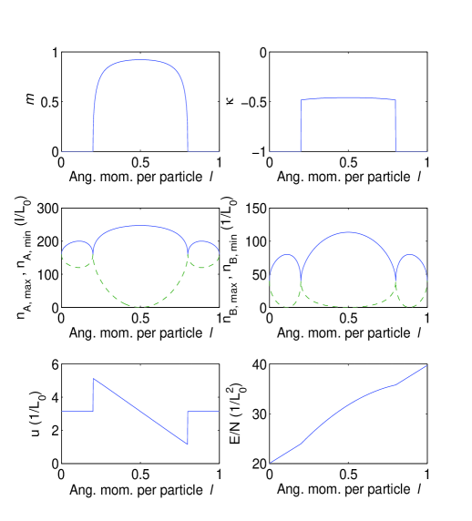
Figure 1: The parameters $m$, $\kappa$, $n_{A,B,{\rm max}}$ (solid line), $n_{A,B,{\rm min}}$ (dashed line), the propagation velocity and the dispersion relation as functions of the angular momentum per particle $l$, for $N_{A}=160$, $N_{B}=40$, and $\gamma_{0}L_{0}=0.2$. For $\ell=1/2$ there is a node in the density of each species (at different points). Also, the velocity of propagation $u$ has a discontinuity at $\ell=x_{A}$ and $\ell=x_{B}$.

One interesting aspect of the periodic gray-bright solution with period equal to $L_{0}$, which is expected to be the yrast state (i.e., the state of minimum energy for some fixed value of the angular momentum), is its size relative to $L_{0}$. A reasonable measure of this size is the ratio of the complex to the real period of the doubly periodic Jacobi solution, since the complex period controls the exponential decay of the solution. In Fig. 2 we plot the ratio of the two periods versus the angular momentum. This ratio becomes infinite when $\ell\to N_{B}/N$, and it has its minimum value when $\ell=1/2$. This suggests that the solution is most localized when $\ell=1/2$. However, even in this case the period ratio is not close to zero, suggesting that the yrast state is not very localized but rather has a size comparable to $L_{0}$ even for strong interatomic interactions. As seen from Fig. 2 when $\gamma_{0}L_{0}=0.2$, i.e., when the ratio between the interaction energy of the homogeneous system and the kinetic energy, $N\gamma_{0}L_{0}/(4\pi^{2})$, is equal to 1, the minimum value of the ratio of the periods is $\approx 0.6$. We have also found numerically that the corresponding minimal ratio for $\gamma_{0}L_{0}=2$, is $\approx 0.37$, suggesting that the size of the waves is comparable to $L_{0}$ even for strong coupling.

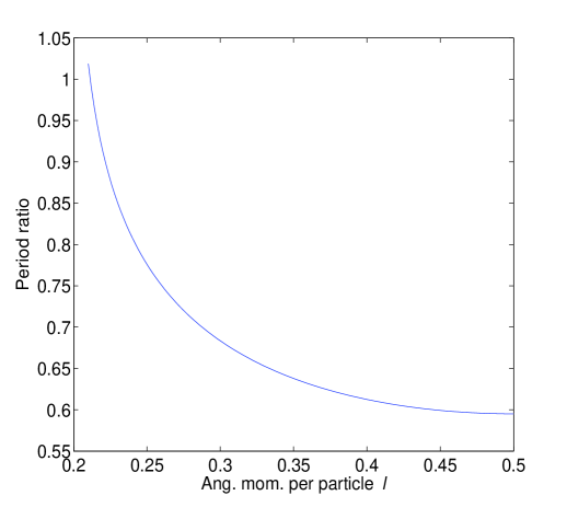
Figure 2: The ratio of the imaginary to the real period of the gray-bright solution for $N_{A}=160$, $N_{B}=40$, and $\gamma_{0}L_{0}=0.2$ as a function of $l$. The period ratio diverges to infinity as $\ell\to N_{B}/N=0.2$. When $\ell=1/2$ we have the minimal ratio, suggesting that we have the most localized solution. However, the ratio is $\approx 0.6$ and thus the size of the localized wave is still approximately two thirds of the size of the period length $L_{0}$.

VII Diagonalization of the Hamiltonian for weak interactions

For sufficiently weak interactions, $\gamma_{0}L_{0}<<1$, it is reasonable to truncate our Hamiltonian to the lowest two angular momentum modes only. Doing this, the second-quantized Hamiltonian becomes

$$\widehat{H}=\frac{1}{2}\left(\frac{2\pi}{L_{0}}\right)^{2}(a_{1}^{\dagger}a_{1}+b_{1}^{\dagger}b_{1})\hskip 80.00012pt$$

$$+\frac{1}{2}\frac{\gamma_{0}}{L_{0}}(a_{0}^{\dagger 2}a_{0}^{2}+b_{0}^{\dagger 2}b_{0}^{2}+a_{1}^{\dagger 2}a_{1}^{2}+b_{1}^{\dagger 2}b_{1}^{2}$$

$$+4a_{0}^{\dagger}a_{1}^{\dagger}a_{0}a_{1}+4b_{0}^{\dagger}b_{1}^{\dagger}b_{0}b_{1}\hskip 55.00008pt$$

$$+2a_{0}^{\dagger}b_{0}^{\dagger}a_{0}b_{0}+2a_{0}^{\dagger}b_{1}^{\dagger}a_{0}b_{1}+2a_{1}^{\dagger}b_{0}^{\dagger}a_{1}b_{0}$$

$$+2a_{1}^{\dagger}b_{1}^{\dagger}a_{1}b_{1}+2a_{1}^{\dagger}b_{0}^{\dagger}a_{0}b_{1}+2a_{0}^{\dagger}b_{1}^{\dagger}a_{1}b_{0}).$$ (84)

We can diagonalize this Hamiltonian by considering the algebra of the bilinears of annihilation-creation operators appearing in it. We define the operators

$$\widehat{n}_{A0} = a_{0}^{\dagger}a_{0},\,\,\widehat{n}_{B0}=b_{0}^{\dagger}b_{0},\,\,\widehat{n}_{A1}=a_{1}^{\dagger}a_{1},\,\,\widehat{n}_{B1}=b_{1}^{\dagger}b_{1},$$

$$\widehat{J}_{A} = a_{1}^{\dagger}a_{0},\,\,\widehat{J}_{A}^{\dagger}=a_{0}^{\dagger}a_{1},\,\,\widehat{J}_{B}=b_{1}^{\dagger}b_{0},\,\,\widehat{J}_{B}^{\dagger}=b_{0}^{\dagger}b_{1}.$$ (85)

The first four operators are the usual number operators. The last four can be used to generate two copies of the ${\rm SU}(2)$ algebra. Since $[\widehat{n}_{A1}-\widehat{n}_{A0},\widehat{J}_{A}]=2\widehat{J}_{A}$, it is natural to define

$$\widehat{J}_{A3}=\frac{1}{2}(\widehat{n}_{A1}-\widehat{n}_{A0}), \widehat{J}_{B3}=\frac{1}{2}(\widehat{n}_{B1}-\widehat{n}_{B0}).$$ (86)

These bilinears can be divided into three sets. One set consists of the operators $\widehat{n}_{A0}+\widehat{n}_{A1}$ and $\widehat{n}_{B0}+\widehat{n}_{B1}$. These operators commute with all other bilinears and are hence central elements. Their eigenvalues are determined by the particle numbers $N_{A}$ and $N_{B}$. The second set consists of the operators $\widehat{J}_{A3}$, $\widehat{J}_{A}$, and $\widehat{J}_{A}^{\dagger}$. The third set consists of the operators $\widehat{J}_{B3}$, $\widehat{J}_{B}$, and $\widehat{J}_{B}^{\dagger}$. The operators in the second set commute with the operators in the third set and the operators in each set satisfy the commutation relations

$$[\widehat{J}_{A3,B3},\widehat{J}_{A,B}]=\widehat{J}_{A,B},\,\,[\widehat{J}_{A3,B3},\widehat{J}_{A,B}^{\dagger}]=-\widehat{J}_{A,B}^{\dagger},$$ (87)

and

$$[\widehat{J}_{A,B},\widehat{J}_{A,B}^{\dagger}]=2\widehat{J}_{A3,B3}.$$ (88)

These are the ${\rm SU}(2)$ commutation relations, which means that the algebra of the bilinears splits into a direct sum of two copies of the ${\rm U}(1)$ algebra and two copies of the ${\rm SU}(2)$ algebra. Note the angular momentum operator can be expressed in terms of these operators as

$$\widehat{L}=\widehat{n}_{A1}+\widehat{n}_{B1}=\frac{1}{2}(N_{A}+N_{B})+(\widehat{J}_{A3}+\widehat{J}_{B3}).$$ (89)

It is now possible to split the Hamiltonian into a central part and an ${\rm SU}(2)$ part, $\widehat{H}=H_{C}+\widehat{H}_{0}$, where

$$H_{C}=\frac{\pi^{2}}{L_{0}^{2}}(N_{A}+N_{B})-\frac{1}{2}\frac{\gamma_{0}}{L_{0}}(N_{A}+N_{B})$$

$$+\frac{3}{4}\frac{\gamma_{0}}{L_{0}}(N_{A}^{2}+N_{B}^{2})+\frac{\gamma_{0}}{L_{0}}N_{A}N_{B},$$ (90)

and

$$\widehat{H}_{0}=\frac{1}{2}\left(\frac{2\pi}{L_{0}}\right)^{2}(\widehat{J}_{A3}+\widehat{J}_{B3})+\frac{\gamma_{0}}{L_{0}}(\widehat{J}_{A}\widehat{J}_{B}^{\dagger}+\widehat{J}_{A}^{\dagger}\widehat{J}_{B}-\widehat{J}_{A3}^{2}-\widehat{J}_{B3}^{2}).$$ (91)

The linear part of $\widehat{H}_{0}$ is can readily be expressed in terms of the angular momentum. Since the Hamiltonian is rotationally symmetric, the quadratic part of $\widehat{H}_{0}$ must commute with the angular momentum. This places significant constraints on the form of the quadratic part of the Hamiltonian. Indeed, if we set $\widehat{J}_{A,B}=\widehat{J}_{A1,B1}+i\widehat{J}_{A2,B2}$ and $\vec{\widehat{J}}_{A,B}=(\widehat{J}_{A1,B1},\widehat{J}_{A2,B2},\widehat{J}_{A3,B3})$, it is possible to rewrite $\widehat{H}_{0}$ in the form

$$\widehat{H}_{0}=\frac{1}{2}\left(\frac{2\pi}{L_{0}}\right)^{2}(\widehat{L}-N/2)-\frac{\gamma_{0}}{L_{0}}(\widehat{L}-N/2)^{2}$$

$$+\frac{\gamma_{0}}{L_{0}}[(\vec{\widehat{J}}_{A}+\vec{\widehat{J}}_{B})^{2}-\vec{\widehat{J}}_{A}^{2}-\vec{\widehat{J}}_{B}^{2}].$$ (92)

Since the angular momentum $\widehat{L}$ depends only on $\widehat{J}_{A3}+\widehat{J}_{B3}$, it commutes with $\vec{\widehat{J}}_{A,B}^{2}$ and with $(\vec{\widehat{J}}_{A}+\vec{\widehat{J}}_{B})^{2}$. Also, since $\widehat{J}_{A3,B3}$ are given in terms of the number operators in Eq. (86), it is clear that their eigenvalues range from $-N_{A,B}/2$ to $N_{A,B}/2$. This means that we are in the spin $j_{A,B}=N_{A,B}/2$ representation of the ${\rm SU}(2)$ algebra. This means that $\vec{\widehat{J}}_{A,B}^{2}$ and $(\vec{\widehat{J}}_{A}+\vec{\widehat{J}}_{B})^{2}$ are given by

$$\vec{J}_{A,B}^{2} = \frac{N_{A,B}}{2}\left(\frac{N_{A,B}}{2}+1\right)\widehat{I}$$ (93)

$$(\vec{J}_{A}+\vec{J}_{B})^{2} = j_{AB}(j_{AB}+1)\widehat{I},$$ (94)

where $\widehat{I}$ stands for the identity operator and $j_{AB}$ ranges from $|j_{A}-j_{B}|=(N_{A}-N_{B})/2$ to $j_{A}+j_{B}=N/2$ as a consequence of the usual rules for the addition of angular momentum. The eigenvalues of the angular momentum operator $\widehat{L}$ are $L=N/2+m_{AB}$, where $m_{AB}$ ranges from $-j_{AB}$ to $j_{AB}$ due to Eq. (89). Therefore, $\widehat{H}_{0}$ can be written in the form

$$\widehat{H}_{0}=\frac{1}{2}\left(\frac{2\pi}{L_{0}}\right)^{2}(\widehat{L}-N/2)-\frac{\gamma_{0}}{L_{0}}(\widehat{L}-N/2)^{2}\hskip 70.0001pt$$

$$+\frac{\gamma_{0}}{L_{0}}\left[j_{AB}(j_{AB}+1)-\frac{N_{A}}{2}\left(\frac{N_{A}}{2}+1\right)-\frac{N_{B}}{2}\left(\frac{N_{B}}{2}+1\right)\right]\widehat{I},$$

(95)

and its eigenvalues are

$$E_{0}=\frac{1}{2}\left(\frac{2\pi}{L_{0}}\right)^{2}(L-N/2)-\frac{\gamma_{0}}{L_{0}}(L-N/2)^{2}$$

$$+\frac{\gamma_{0}}{L_{0}}[j_{AB}(j_{AB}+1)-\frac{N_{A}}{2}\left(\frac{N_{A}}{2}+1\right)-\frac{N_{B}}{2}\left(\frac{N_{B}}{2}+1\right)].$$

(96)

Adding to this the contribution from $H_{C}$ we get that the energy eigenvalues are

$$E=-\frac{\gamma_{0}}{L_{0}}L^{2}+\frac{1}{2}\left(\frac{2\pi}{L_{0}}\right)^{2}L+\frac{\gamma_{0}}{L_{0}}NL+\frac{1}{2}\frac{\gamma_{0}}{L_{0}}N(N-1)$$

$$-\frac{1}{2}\frac{\gamma_{0}}{L_{0}}N_{A}N_{B}+\frac{\gamma_{0}}{L_{0}}[j_{AB}(j_{AB}+1)-\frac{N_{A}}{2}\left(\frac{N_{A}}{2}+1\right)$$

$$-\frac{N_{B}}{2}\left(\frac{N_{B}}{2}+1\right)].$$

(97)

It is now possible to determine the yrast energy. Since $L=N/2+m_{AB}$, the value of $m_{AB}$ is completely determined, and the minimum energy is obtained for the minimum value of $j_{AB}$. For $0<L<N_{B}$, $-N/2<m_{AB}<-(N_{A}-N_{B})/2$, and the minimum value of $j_{AB}$ is $|m_{AB}|=N/2-L$. Substituting this value of $j_{AB}$ into Eq. (97) yields

$$E_{0<L<N_{B}}^{\rm gr}=\frac{1}{2}\left(\frac{2\pi}{L_{0}}\right)^{2}L+\frac{\gamma_{0}}{L_{0}}\left(\frac{1}{2}N(N-1)-L\right).$$ (98)

The excited energy levels are given by Eq. (97), with $N/2-L<j_{AB}\leq N/2$.

For $N_{B}<L<N_{A}$ the minimum value of $j_{AB}$ is by $(N_{A}-N_{B})/2$, independent of $L$. In this case the minimum energy is

$$E_{N_{B}<L<N_{A}}^{\rm gr}=\frac{1}{2}\left(\frac{2\pi}{L_{0}}\right)^{2}L+\frac{\gamma_{0}}{L_{0}}\left(\frac{1}{2}N(N-1)\right.$$

$$\left.-N_{A}N_{B}-N_{B}-L^{2}+NL\right).$$ (99)

The energy levels of the excited states are given by Eq. (97) with $(N_{A}-N_{B})/2<j_{AB}\leq N/2$.

For $N_{A}<L<N$, $(N_{A}-N_{B})/2<m_{AB}<N/2$, and the minimum value of $j_{AB}$ is $m_{AB}=L-N/2$. Substitution into Eq. (97) now gives

$$E_{N_{A}<L<N}^{\rm gr}=\frac{1}{2}\left(\frac{2\pi}{L_{0}}\right)^{2}L+\frac{\gamma_{0}}{L_{0}}\left(\frac{1}{2}N(N-1)-N+L\right).$$ (100)

The excited energy levels are again given by Eq. (97) with $L-N/2<j_{AB}\leq N/2$.

VIII Conclusions

The issue of finding solitary-wave solutions of the nonlinear Schrödinger equation is an old problem with varying degrees of difficulty. The most elementary question is that of a single component which extends to infinity. The case of a single component with periodic boundary conditions introduces some interesting complications. In the presence of a second component, the similar questions introduce additional complications, as there are now two coupled equations. Here we have considered the case of solitary-wave solutions in a two-component Bose-Einstein condensed gas, which is confined to a zero width (i.e., one dimensional) ring of finite radius, therefore requiring the imposition of periodic boundary conditions.

Within the mean-field approximation and with the use of a reasonable ansatz for the solution, we have integrated the coupled nonlinear equations describing order parameters to find two analytic solutions which can be expressed in terms of Jacobi elliptic functions.

This problem is also connected to the determination of the yrast state, i.e., the state of lowest energy state solution given some fixed value of the expectation value of the angular momentum. We have shown explicitly that the yrast state for this problem is the gray-bright solution, in accordance with general arguments equiv . The corresponding phase winding numbers that describe the global minima depend on the angular momentum of the system, giving rise in this way to various sectors of the dispersion relation, which nevertheless remains continuous. For weak coupling, this is shown analytically, however the numerical solution of the constraints suggests that the situation does not change qualitatively for stronger couplings.

Going beyond the mean-field approximation, we have also diagonalized the many-body Hamiltonian exactly in the limit of weak interactions, which allows us to truncate the Hamiltonian to the two lowest-angular momentum modes. We have thus managed to derive the entire excitation spectrum of this many-body system, which in a sense corresponds to a “quantum” solitary-wave solution.

Ideally we would like to find solutions for arbitrary masses $M_{A}$ and $M_{B}$, for arbitrary coupling constants $\gamma_{AA}$, $\gamma_{BB}$, and $\gamma_{AB}$, and for arbitrary $u$. We have found analytic solutions by imposing the “artificial” constraints that $M_{A}=M_{B}$ and $\gamma_{AA}=\gamma_{BB}=\gamma_{AB}$. We expect that small violations of these constraints would lead to new (linear) equations that would be non-singular and well-behaved. This suggests that the present constrained solutions are broadly representative of all solutions which do not violate the constraints “violently”.

Appendix 1

Let us consider the expansion of the gray-bright solution when $m$ is close to zero. The Lambert series for the Jacobi elliptic functions tell us that, for $q(m)$ close to 1,

$${\rm sn}(\frac{2K(m)z}{L_{0}}|m)\sim\frac{2\pi}{K(m)\sqrt{m}}\left(\frac{q(m)^{1/2}}{1-q(m)}\sin(\frac{\pi z}{L_{0}})\right.$$

$$\left.+\frac{q(m)^{3/2}}{1-q(m)^{3}}\sin(\frac{3\pi z}{L_{0}})+\cdots\right),$$ (101)

where $q(m)$ is the nome function. Its expansion for small $m$ is

$$q(m)=\frac{m}{16}+\frac{m^{2}}{32}+{\cal O}(m^{3}).$$ (102)

Making use of the the expansion of the first elliptic integral $K(m)$,

$$K(m)=\frac{\pi}{2}\left(1+\frac{1}{4}m+\frac{9}{64}m^{2}+O(m^{3})\right),$$ (103)

we find that

$${\rm sn}(\frac{2K(m)z}{L_{0}}|m)\sim\sin(\frac{\pi z}{L_{0}})+$$

$$+\frac{m}{16}(\sin(\frac{\pi z}{L_{0}})+\sin(\frac{3\pi z}{L_{0}}))+{\cal O}(m^{2}).$$ (104)

Similarly, we find

$${\rm cn}(\frac{2K(m)z}{L_{0}}|m)\sim\cos(\frac{\pi z}{L_{0}})+$$

$$+\frac{m}{16}(-\cos(\frac{\pi z}{L_{0}})+\cos(\frac{3\pi z}{L_{0}}))+{\cal O}(m^{2}).$$ (105)

Expansions similar to Eq. (103) also exist for the second and the third elliptic integrals,

$$E(m)=\frac{\pi}{2}\left(1-\frac{1}{4}m-\frac{3}{64}m^{2}+{\cal O}(m^{3})\right),$$ (106)

and

$$\Pi(a|m)=\frac{\pi}{2\sqrt{1-a}}+\frac{\pi m}{4a}\left(\frac{1}{\sqrt{1-a}}-1\right)$$

$$-\frac{\pi m^{2}}{32a}\left(3a-\frac{6}{\sqrt{1-a}}+6\right)+{\cal O}(m^{3}).$$ (107)

Appendix 2

We wish to evaluate the integral appearing in Eq. (39). In doing this we will use the integrals

$$\int_{-K(m)}^{K(m)}{\rm sn}^{2}(u|m)du = \frac{2(K(m)-E(m))}{m},$$ (108)

$$\int_{-K(m)}^{K(m)}{\rm sn}^{4}(u|m)du = \frac{2[(m+2)K(m)-2(m+1)E(m)]}{3m^{2}}.$$

Recalling that the solution ansatz tells us that $n_{B}=\kappa n_{A}+\lambda$, the normalization condition gives $\lambda=(N_{B}-\kappa N_{A})/L_{0}$. Making this substitution in Eq. (39), we obtain

$$E_{0}=\gamma_{0}\Big{[}(1+\kappa)^{2}\int_{-L_{0}/2}^{L_{0}/2}n_{A}^{2}dz+\frac{N_{A}N_{B}}{L_{0}}-\frac{3}{2}\kappa\frac{N_{A}^{2}}{L_{0}}$$

$$-\kappa^{2}\frac{N_{A}^{2}}{L_{0}}+\frac{N_{B}^{2}}{L_{0}}+\frac{1}{2\kappa}\frac{N_{B}^{2}}{L_{0}}\Big{]}.\hskip 20.00003pt$$ (110)

The particle normalization condition can be used to reduce the remaining integral to

$$\int_{-L_{0}/2}^{L_{0}/2}{\rm sn}^{2}(\frac{2K(m)z}{L_{0}}|m)dz=\frac{L_{0}}{m}(1-\frac{E(m)}{K(m)})$$

$$=\frac{N_{A}-n_{A,{\rm min}}L_{0}}{n_{A,{\rm max}}-n_{A,{\rm min}}}.\hskip 80.00012pt$$ (111)

The normalization condition also enables to eliminate the ratio $E(m)/K(m)$ to obtain

$$\int_{-L_{0}/2}^{L_{0}/2}{\rm sn}^{4}(\frac{2K(m)z}{L_{0}}|m)dz$$

$$=\frac{L_{0}}{3m^{2}}\Big{[}(m+2)-2(m+1)\frac{E(m)}{K(m)}\Big{]}=$$

$$\frac{L_{0}}{3m}\Big{[}-1+2(m+1)\frac{N_{A}/L_{0}-n_{A,{\rm min}}}{n_{A,{\rm max}}-n_{A,{\rm min}}}\Big{]}.$$ (112)

Substituting Eqs. (111) and (112) into Eq. (110), we obtain Eq. (40).

References

• (1) S. Burger, K. Bongs, S. Dettmer, W. Ertmer, K. Sengstock, A. Sanpera, G. V. Shlyapnikov, and M. Lewenstein, Phys. Rev. Lett. 83, 5198 (1999).
• (2) J. Denschlag, J. E. Simsarian, D. L. Feder, Charles W. Clark, L. A. Collins, J. Cubizolles, L. Deng, E. W. Hagley, K. Helmerson, W. P. Reinhardt, S. L. Rolston, B. I. Schneider, and W. D. Phillips, Science 287, 97 (2000).
• (3) K. E. Strecker, G. B. Partridge, A. G. Truscott, and R. G. Hulet, Nature (London) 417, 150 (2002).
• (4) L. Khaykovich, F. Schreck, G. Ferrari, T. Bourdel, J. Cubizolles, L. D. Carr, Y. Castin, and C. Salomon, Science 296, 1290 (2002).
• (5) Christoph Becker, Simon Stellmer, Parvis Soltan-Panahi, Sören Dörscher, Mathis Baumert, Eva-Maria Richter, Jochen Kronjäger, Kai Bongs, and Klaus Sengstock, Nature Phys. 4, 496 (2008).
• (6) T. Tsuzuki, J. Low Temp. Phys. 4, 441 (1971).
• (7) V. E. Zakharov and A. B. Shabat, Zh. Eksp. Teor. Fiz. 64, 1627 (1973) [Sov. Phys. JETP 37, 823 (1973)].
• (8) L. D. Carr, C. W. Clark, and W. P. Reinhardt, Phys. Rev. A 62, 063610 (2000).
• (9) J. Smyrnakis, M. Magiropoulos, G. M. Kavoulakis, and A. D. Jackson, Phys. Rev. A 82, 023604 (2010).
• (10) E. Lieb, Phys. Rev. 130, 1616 (1963).
• (11) P. P. Kulish, S. V. Manakov, and L. D. Faddeev, Theor. Math. Phys. 28, 615 (1976); M. Ishikawa and H. Takayama, J. Phys. Soc. Jpn. 49, 1242 (1980).
• (12) S. Trillo, S. Wabnitz, E. M. Wright, and G. I. Stegeman, Opt. Lett. 13, 871 (1988).
• (13) D. N. Christodoulides, Phys. Lett. A 132, 451 (1988).
• (14) M. Shalaby and A. J. Barthelemy, IEEE J. Quantum Electron. 28, 2736 (1992).
• (15) P. Ohberg and L. Santos, Phys. Rev. Lett. 86, 2918 (2001).
• (16) T. Busch and J. R. Anglin, Phys. Rev. Lett. 87, 010401 (2001).
• (17) P. G. Kevrekidis, H.E. Nistazakis, D. J. Frantzeskakis, B. A. Malomed, and R. Carretero-Gonzalez, Eur. Phys. J. D 28, 181 (2004).
• (18) N. G. Berloff, Phys. Rev. Lett. 94, 120401 (2005).
• (19) V. A. Brazhnyi and V. V. Konotop, Phys. Rev. E 72, 026616 (2005).
• (20) X. Liu, H. Pu, B. Xiong, W. M. Liu, and J. Gong, Phys. Rev. A 79, 013423 (2009).
• (21) S. V. Manakov, Sov. Phys. JETP 38, 248 (1974).
• (22) J. Smyrnakis, M. Magiropoulos, A. D. Jackson, and G. M. Kavoulakis, e-print arXiv:1203.2020.
• (23) J. Smyrnakis, S. Bargi, G. M. Kavoulakis, M. Magiropoulos, K. Karkkainen, and S. M. Reimann, Phys. Rev. Lett. 103, 100404 (2009).
• (24) R. Kanamoto, L. D. Carr, and M. Ueda, Phys. Rev. A 81, 023625 (2010).
• (25) A. D. Jackson, J. Smyrnakis, M. Magiropoulos, and G. M. Kavoulakis, Europh. Lett. 95, 30002 (2011).
• (26) F. Bloch, Phys. Rev. A 7, 2187 (1973).