Phylogenetic confidence intervals for the optimal trait value
Krzysztof Bartoszek and Serik Sagitov
Abstract
We consider a stochastic evolutionary model for a phenotype developing amongst
related species with unknown phylogeny.
The unknown tree is modelled by a Yule process conditioned on
contemporary nodes.
The trait value is assumed to evolve along lineages as an Ornstein–Uhlenbeck process.
As a result, the trait values of the species form a sample with dependent observations.
We establish three limit theorems for the sample mean corresponding to three domains for the
adaptation rate.
In the case of fast adaptation, we show that for large the normalized sample mean is
approximately normally distributed.
Using these limit theorems, we develop novel confidence interval formulae for the optimal
trait value.
Phylogenetic comparative methods deal with multi-species trait value data.
This is an established and rapidly expanding area of research concerning evolution of phenotypes in groups of
related species living under various environmental conditions. An important feature of such data is the
branching structure of evolution causing dependence among the observed trait values.
For this reason the usual starting point for phylogenetic comparative studies is an inferred phylogeny
describing the evolutionary relationships. The likelihood can be computed by assuming a model for trait
evolution along the branches of this fixed tree, such as the Ornstein-Uhlenbeck process.
The one-dimensional Ornstein-Uhlenbeck model is characterized by four parameters: the optimal value ,
the adaptation rate , the ancestral value , and the noise size .
The classical Brownian motion model [14] can be viewed as a special case with and
being irrelevant. As with any statistical procedure, it is important to be able to compute confidence
intervals for these parameters. However, confidence intervals are often not mentioned in
phylogenetic comparative studies [8].
There are a number of possible numerical ways of calculating such confidence intervals when the underlying
phylogenetic tree is known.
Using a regression framework one can apply standard regression theory methods to compute confidence
intervals for conditionally on [15, 20, 28, 33].
Notably in [16] the authors derive analytical formulae for confidence intervals for under the
Brownian motion model.
In more complicated situations a parametric bootstrap is a (computationally very demanding) way out
[8, 11, 27]. Another approach
is to report a support surface [20, 21], or consider the curvature of the
likelihood surface [7].
All of the above methods have in common that they assume that the phylogeny describing the evolutionary
relationships is fully resolved.
Possible errors in the topology can cause problems – the closer to the tips they occur, the more problematic they can be
[43].
On the other hand, the regression estimators will remain unbiased even with a misspecified
tree [34] and also seem to be robust with respect to errors in the phylogeny
at least for the Brownian motion model [42]. There are only few papers addressing the issue of
phylogenetic uncertainty.
An MCMC procedure to jointly estimate the phylogeny and parameters of the
Brownian model of trait evolution was suggested in [26, 25].
Recently, [36] develops an Approximate Bayesian Computation framework to estimate
Brownian motion parameters in the case of an incomplete tree.
Our paper studies a situation when nothing is known about the phylogeny. The simplest stochastic model addressing
this case is a combination of a Yule tree and the Brownian motion on top of it:
already in the 1970s, a
joint maximum likelihood estimation procedure of a Yule tree and Brownian motion on top of
it was proposed
in [13]. This basic evolutionary model allows for far reaching analytical analysis
[6, 12, 35].
A more realistic stochastic model of this kind combines the Brownian motion with a birth-death tree allowing for
extinction of species [10]. For the latter model [35] explicitly compute the
so-called
interspecies correlation coefficient.
Such “tree-free” models are appropriate for working with fossil data when there may be available rich fossilized
phenotypic information but the
molecular material might have degraded so much that it is impossible to infer evolutionary relationships.
In [12] the usefulness of the tree-free approach for contemporary species
is demonstrated in an Carnivora order case study and in [31] the distribution
over the space of Yule trees of the interspecies correlation coefficient is calculated.
Conditioned birth–death processes as stochastic models for species trees,
have received significant attention in the last decade
[3, 18, 29, 38, 39, 40].
In this work the unknown tree is modeled by the Yule process conditioned on extant species while the
evolution of a trait along a lineage is viewed as the Ornstein-Uhlenbeck process, see Fig. 1.
We study the properties of the sample mean and sample variance computed from the vector of trait values.
Our main results are three asymptotic confidence interval formulae for the optimal trait value .
These three formulae represent three asymptotic regimes for different values of the adaptation rate .
In the discussion in [12] it is pointed out that “as evolutionary biologists further refine our
knowledge of
the tree of life, the number of clades whose phylogeny is truly unknown may diminish, along with
interest in tree-free estimation methods.” In our opinion the main contribution
of such methods is that they indicate statistical and asymptotic properties of phylogenetic samples
under given evolutionary models. These properties can then be verified for
other models of tree growth or real phylogenies
[4, 5, 17, 22, 23, 24, 30].
We believe furthermore that
the easy-to-compute tree-free predictions
will always play an important role of a sanity check to see
whether the conclusions based on the inferred phylogeny deviate much from those
from a “typical” phylogeny.
Moreover, results like those presented here can also be used as a method of testing
software for phylogenetic comparative models.
A detailed description of the evolutionary model along with our
main results are presented in Section
2. Section 3 contains new formulae for the Laplace transforms of important
characteristics of the conditioned Yule species tree: the time to origin and the time to the most
recent common ancestor for a pair of two species chosen at random out of extant species.
In Section 4 we calculate the interspecies correlation coefficient for the Yule–Ornstein–Uhlenbeck model
and Section 5 contains the proof of our limit theorems.
In Section 6 we establish the consistency of the stationary variance estimator,
which is needed for our confidence interval formulae, cf [20] where
the residual sum of squares was suggested to estimate the stationary variance.
In Appendix A we calculate all the joint moments of and .
Our main result, Theorem 2.1, should be compared with the limit theorems obtained in
[1, 2]. They also revealed three asymptotic regimes in a related,
though different setting,
dealing with a branching Ornstein–Uhlenbeck process. In their case the time of observation is
deterministic and the number of the tree tips is random, while in our case the observation time is
random and the number of the tips is deterministic. Although it is possible (with some effort)
to deduce our results from [1, 2], our proof provides a much more
elementary derivation. We believe that our approach will be useful in addressing other biologically
relevant issues like the formulae for the higher moments given in Appendix A.
Another similar limit theorem, but one conditional on the sequence of species trees
generated by different mechanisms,
is derived in [5].
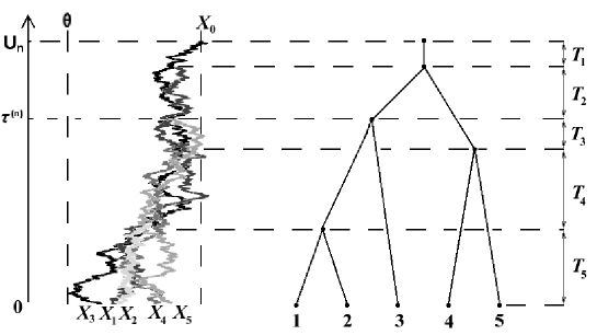
Figure 1:
On the left: a branching Ornstein–Uhlenbeck process simulated on a realization of the Yule -tree with tips using the
TreeSim [38, 39] and mvSLOUCH [7] R [32] packages.
Parameters used are , , , after the tree height was scaled to 1.
On the right: the species tree disregarding the trait values supplied with the notation for the inter–speciation times.
For the pair of tips (2,3) the time to their most recent common ancestor is marked on the time axis
(starting at present and going back to the time of origin).
2 The model and main results
This work deals with what we call the Yule–Ornstein–Uhlenbeck model which is characterized by four parameters and consists of two ingredients
1.
the species tree connecting extant species is modeled by the pure birth Yule process [44] with
a unit speciation rate and conditioned on having tips [18],
2.
the observed trait values on the tips of the tree evolved from the ancestral state following the
Ornstein–Uhlenbeck process with parameters .
Definition 2.1
Let be independent exponential random variables with parameters . We define the Yule -tree as a random tree with tips which is
constructed using a bottom-up algorithm based on the following two simple rules.
(1) During the time period the tree has branches.
(2) For the reduction from to branches occurs as two randomly chosen branches
coalesce into one branch.
The height the Yule -tree is now .
As shown in [18], this definition corresponds to the standard Yule tree conditioned on having tips at the moment of observation, assuming that the time to the origin has the improper uniform prior.
Following [11, 20], we model trait evolution along a lineage using the Ornstein–Uhlenbeck process given by the stochastic differential equation
(1)
Here is the adaptation rate, is the optimal trait value, is the noise variance, and is the standard Wiener process.
The distribution of is normal with,
(2)
implying that looses the effect of the ancestral state at an exponential rate.
In the long run the Ornstein–Uhlenbeck process acquires a stationary normal distribution with mean and variance .
We propose asymptotic confidence interval formulae for the optimal value which take into account phylogenetic uncertainty. To this end we study properties of the sample mean and sample variance
Using the properties of the Yule–Ornstein–Uhlenbeck model we find explicit expressions for , , ,
study the asymptotics of , and prove the following limit theorem revealing three different asymptotic regimes.
Theorem 2.1
Let be a normalized difference between the ancestral and optimal values.
Consider the normalized sample mean
of the Yule-Ornstein-Uhlenbeck process with . As the process has the following limit behavior.
(i) If , then is asymptotically normally distributed with zero mean and variance
.
(ii) If , then is asymptotically normally distributed with zero mean and variance .
(iii) If , then
converges a.s. and in to a random variable with and .
Let be the -quantile of the standard normal distribution, and be the -quantile of the limit . Denote by the sample standard deviation defined as the square root of . As it will be shown in Section 6, the sample variance is a consistent estimator of . This fact together with Theorem 2.1 allows us to state the following three approximate
-level confidence intervals for assuming that we know the value of :
Notably, the first of these confidence intervals differs from the classical confidence interval for the mean
just by a factor . The latter is larger than 1, as it should, in view of a positive correlation among the
sample observations. The correction factor becomes negligible in the case of a very strong adaptation,
, when the dependence due to common ancestry can be neglected.
Remark 2.1
Observe that our standing assumption , see Definition 2.1, of
having one speciation event per unit of time causes no loss of generality.
To incorporate an arbitrary speciation rate one has to replace in our
formulae parameters and by and .
This transformation corresponds to the time scaling by factor in Eq. (1),
it changes neither the optimal value nor the stationary variance .
3 Sampling leaves from the Yule -tree
Here we consider the Yule -tree, see Definition 2.1 and study some properties of its
subtree joining randomly (without replacement) chosen tips, where .
In particular, we compute the joint Laplace
transform of the height of the Yule -tree
and ,
the height of the most recent common ancestor for two randomly sampled tips, see Fig. 1.
For other results concerning the distribution of and see also
[18, 19, 29, 35, 37, 38, 40, 41].
Lemma 3.1
Consider a random -subtree of the conditioned Yule -tree. It has
bifurcating events.
Let be the
consecutive numbers of the bifurcation events in the Yule -tree (counted from the root toward the leaves)
corresponding to the bifurcating events of the -subtree. Put and .
The sequence forms a time inhomogeneous Markov chain with transition probabilities
where for all , and
Proof
Tracing the lineages of randomly sampled tips of the Yule -tree towards the root,
the first coalescent event can be viewed as the success in a sequence of independent Bernoulli trials.
This argument leads to the expression cf [38]
confirming the formula stated for the transition probabilities . The transition probabilities for are obtained similarly. Notice, as a check, that .
Lemma 3.2
Consider the inter-bifurcation times for the -subtree of the Yule -tree
so that for any , and .
Then for we have
where , , and
Proof
The Laplace transform of the sum of independent exponentials:
together with Lemma 3.1 implies the stated equality
Lemma 3.3
The joint Laplace
transform of the height of the Yule -tree
and
the height of the most recent common ancestor for two randomly sampled tips is given by
This implies the main formula claimed by Lemma 3.3 giving after putting .
With ,
When this directly becomes
In the case of we use the following relation (easily verified by induction when )
(9)
to derive
Lemma 3.4
As for positive and we have the following asymptotic results
where
Proof
The stated results are obtained from Lemma 3.3 using the first of the following three asymptotic properties of the function
These three relations will often be used tacitly in what follows.
4 Interspecies correlation
Denote by the –algebra containing all information on the Yule -tree.
The scaled trait values , in view of Eq. (2), are conditionally
normal with
which together with the results from Section 3 entails
Lemma 4.1
In the framework of the Yule-Ornstein-Uhlenbeck model, for an arbitrary pair of traits we have
where is the backward time to the most recent common ancestor of the tips .
Proof
Denote by the normalized trait value of the most recent common ancestor of the tips .
Let stand for the –algebra generated by , then using Eq. (2) we get
implying the statement of this lemma
Lemma 4.2
Consider the interspecies correlation coefficient, the unconditioned correlation between two randomly sampled trait values
Applying the results of Section 3 we arrive at the asserted relations for . Observe that asymptotically as the interspecies correlation coefficient decays to as
Lemma 4.3
Consider the sample mean and the sample variance
of the scaled trait values. For all we have . For
and in the singular case
Proof
Obviously, .
To prove the other assertions we turn to [35], where the concept of interspecies correlation was originally introduced. It was shown there that the variance of the sample average and the expectation
of the sample variance can be compactly expressed as
Since , , and
it remains to combine Lemma 4.2 with the known expression for .
A more direct proof of Lemma 4.3 can be obtained using the following result on conditional expectations.
Put
with .
For any the sequence forms a martingale
converging a.s. and in .
Moreover, converges in distribution to a random variable having the
standard Gumbel distribution.
Proof
The martingale property is obvious
Since the second moments
are uniformly bounded over , we may conclude that a.s. and in
with .
It follows that , and therefore, . The latter is a convergence of Laplace transforms confirming the stated
convergence in distribution.
Observe that the Gumbel limit for can be obtained using the
classical extreme value theory, in view of the representation
in terms of independent exponentials with parameter 1.
Notice also that has the same distribution as the total branch length of Kingman’s -coalescent.
Lemma 5.2
Denote by the –algebra containing information on the Yule -tree realization
as well as the corresponding information on the evolution of trait values. Set
The sequence forms a martingale with .
Proof
Notice that,
Hence
Lemma 5.3
For all positive we have
as .
Proof
For a given realization of the Yule -tree we denote by and two independent versions of corresponding to two independent choices of pairs of tips out of available. We have,
Taking the difference between the last two expressions we find
Using the simple equality
we see that it suffices to prove that,
where
To verify these two asymptotic relations observe that
Since
,
it follows
and
Proof of Theorem 2.1 (i) and (ii).
Let . To establish the stated normal approximation it is enough to prove the convergence in probability of the first two conditional moments
since then, due to the conditional normality of , we will get the following convergence of characteristic functions
It remains to observe that on one hand, according to Lemma 5.3
and on the other hand, , implying that . This together with holding in and therefore in probability, entails , finishing the proof of part (i).
Part (ii) is proven similarly.
Proof of Theorem 2.1 (iii). Let . Turning to Lemma 5.2 observe that the martingale has uniformly bounded second moments. Indeed, due to Lemma 4.4
Thus, according to Lemma 3.4 we have . Referring to the martingale -convergence theorem we conclude that almost surely and in . Due to Lemma 5.1 it follows that
Finally, as
6 Consistency of the sample variance
Recall that , and according to Lemma 4.3 we have . The aim of this section is to show that as which is equivalent to
(10)
To this end we will need the following formula, see Eq. (13) in [9]
valid for any normally distributed vector with means and covariances
:
In the special case with it follows
(11)
Writing instead of we use the representation
to find out that
Denoting by a random sample without replacement of four trait values out of available, so that
we derive
(12)
We compute the five fourth-order moments in the last expression using the conditional normality of the random quadruple
with conditional moments given by
where is the time to the most recent ancestor for the pair of tips among randomly chosen tips of the Yule -tree. Clearly, all have the same distribution as , and for
Using an estimate for similar to that we used in (iv), we find as .
Finally, putting the above results (i) - (v) into Eq. (12) we arrive at Eq. (10).
Acknowledgments
We are grateful to Thomas F. Hansen and Anna Stokowska for helpful suggestions and comments. Special thanks to an anonymous referee for the constructive suggestions to the earlier version of the paper, in particular, for the remark added after Lemma 5.1.
The research of Serik Sagitov was supported by the Swedish Research Council grant 621-2010-5623.
Krzysztof Bartoszek was supported by the Centre for Theoretical Biology at the University of Gothenburg,
Svenska Institutets Östersjösamarbete
scholarship nr. 11142/2013,
Stiftelsen för Vetenskaplig Forskning och Utbildning i Matematik
(Foundation for Scientific Research and Education in Mathematics),
Knut and Alice Wallenbergs travel fund, Paul and Marie Berghaus fund, the Royal Swedish Academy of Sciences,
and Wilhelm and Martina Lundgrens research fund.
Appendix A
All moments of and
Eq. (3) for the Laplace transforms of the random
variable can be used to calculate the moments of using,
(13)
For a fixed we introduce the following notation,
Notice that
and is the –th generalized harmonic number of order ,
(14)
We can write Eq. (3) as . Its first derivative with respect
to is , and the second derivative is .
For the general recursive formula we introduce the following notation.
We will denote by
infinite dimensional vectors with integer–valued components, and write if all and .
Therefore represents the set of all possible ways to represent as a sum of positive integers. We will also
use the multi–index notation
.
Since ,
and , we can show by induction that,
(15)
where coefficients are defined for all vectors with integer–valued components using the recursion,
(16)
with and
The boundary conditions for the recursion of Eq. (16) consist of two parts:
•
, if all , or one of the coordinates of the vector is negative,
The technique for calculating the –th derivative of the Laplace
transform of given by Eq. (7) is the same but requires new notation
Notice that ,
,
and if is even or if is odd.
One can then inductively show that,
with the coefficients defined as previously by Eq. (16).
Therefore, we get,
Similarly we can use Eq. (3) to calculate the joint moments for and in terms of,
For and we first get,
and then from the above,
References
Adamczak and Miłoś [2011]
R. Adamczak and P. Miłoś.
CLT for Ornstein–Uhlenbeck branching particle system.
ArXiv e-prints, 2011.
Adamczak and Miłoś [in press]
R. Adamczak and P. Miłoś.
U–statistics of Ornstein–Uhlenbeck branching particle system.
J. Th. Probab., in press.
Aldous and Popovic [2005]
D. Aldous and L. Popovic.
A critical branching process model for biodiversity.
Adv. Appl. Probab., 37(4):1094–1115,
2005.
Ané [2008]
C. Ané.
Analysis of comparative data with hierarchical autocorrelation.
Ann. Appl. Stat., 2(3):1078–1102, 2008.
Ané et al. [2014]
C. Ané, L. S. T. Ho, and S. Roch.
Phase transition on the convergence rate of parameter estimation
under an Ornstein–Uhlenbeck diffusion on a tree.
ArXiv e-prints, 2014.
Bartoszek [2014]
K. Bartoszek.
Quantifying the effects of anagenetic and cladogenetic evolution.
Math. Biosc., 254:42–57, 2014.
Bartoszek et al. [2012]
K. Bartoszek, J. Pienaar, P. Mostad, S. Andersson, and T. F. Hansen.
A phylogenetic comparative method for studying multivariate
adaptation.
J. Theor. Biol., 314:204–215, 2012.
Boettiger et al. [2012]
C. Boettiger, G. Coop, and P. Ralph.
Is your phylogeny informative? Measuring the power of comparative
methods.
Evolution, 2012.
Bohrnstedt and Goldberger [1969]
G. W. Bohrnstedt and A. S. Goldberger.
On the exact covariance of products of random variables.
J. Am. Stat. Assoc., 64:1439–1442, 1969.
Bokma [2010]
F. Bokma.
Time, species and seperating their effects on trait variance in
clades.
Syst. Biol., 59(5):602–607, 2010.
Butler and King [2004]
M. A. Butler and A. A. King.
Phylogenetic comparative analysis: a modelling approach for adaptive
evolution.
Am. Nat., 164(6):683–695, 2004.
Crawford and Suchard [2013]
F. W. Crawford and M. A. Suchard.
Diversity, disparity, and evolutionary rate estimation for unresolved
Yule trees.
Syst. Biol., 62(3):439–455, 2013.
Edwards [1970]
A. W. F. Edwards.
Estimation of the branch points of a branching diffusion process.
J. Roy. Stat. Soc. B, 32(2):155–174,
1970.
Felsenstein [1985]
J. Felsenstein.
Phylogenies and the comparative method.
Am. Nat., 125(1):1–15, 1985.
Garland and Ives [2000]
T. Garland and A. R. Ives.
Using the past to predict the present: Confidence intervals for
regression equations in phylogenetic comparative methods.
Am. Nat., 155(3):346–364, 2000.
Garland et al. [1999]
T. Garland, P. E. Midford, and A. R. Ives.
An introduction to phylogenetically based statistical methods, with a
new method for confidence intervals on ancestral values.
Amer. Zool., 39:374–388, 1999.
Gascuel and Steel [2014]
O. Gascuel and M. Steel.
Predicting the ancestral character changes in a tree is typically
easier than predicting the root state.
Syst. Biol., 63(3):421–435, 2014.
Gernhard [2008a]
T. Gernhard.
The conditioned reconstructed process.
J. Theor. Biol., 253:769–778, 2008a.
Gernhard [2008b]
T. Gernhard.
New analytic results for speciation times in neutral models.
B. Math. Biol., 70:1082–1097, 2008b.
Hansen [1997]
T. F. Hansen.
Stabilizing selection and the comparative analysis of adaptation.
Evolution, 51(5):1341–1351, 1997.
Hansen et al. [2008]
T. F. Hansen, J. Pienaar, and S. H. Orzack.
A comparative method for studying adaptation to a randomly evolving
environment.
Evolution, 62:1965–1977, 2008.
Ho and Ané [2013]
L. S. T. Ho and C. Ané.
Asymptotic theory with hierarchical autocorrelations:
Ornstein–Uhlenbeck tree models.
Ann. Stat., 41(2):957–981, 2013.
Ho and Ané [2014]
L. S. T. Ho and C. Ané.
A linear–time algorithm for Gaussian and non-Gaussian trait
evolution models.
Syst. Biol., 63(3):397–408, 2014.
Ho and Ané [in press]
L. S. T. Ho and C. Ané.
Intrinsic inference difficulties for trait evolution with
Ornstein–Uhlenbeck models.
Meth. Ecol. Evol., in press.
Huelsenbeck and Rannala [2003]
J. P. Huelsenbeck and B. Rannala.
Detecting correlation between characters in a comparative analysis
with uncertain phylogeny.
Evolution, 57(6):1237–1247, 2003.
Huelsenbeck et al. [2000]
J.P. Huelsenbeck, B. Rannala, and J.P. Masly.
Accommodating phylogenetic uncertainty in evolutionary studies.
Science, 88:2349–2350, 2000.
Ives et al. [2007]
A. R. Ives, P. E. Midford, and T. Garland.
Within–species variation and measurement error in phylogenetic
comparative methods.
Syst. Biol., 56(2):252–270, 2007.
Martins and Hansen [1997]
E. P. Martins and T. F. Hansen.
Phylogenies and the comparative method: a general approach to
incorporating phylogenetic information into the analysis of interspecific
data.
Am. Nat., 149(4):1341–1351, 1997.
Mooers et al. [2012]
A. Mooers, O. Gascuel, T. Stadler, H. Li, and M. Steel.
Branch lengths on birth–-death trees and the expected loss of
phylogenetic diversity.
Syst. Biol., 61(2):195–203, 2012.
Mossel and Steel [2014]
E. Mossel and M. Steel.
Majority rule has transition ratio 4 on Yule trees under a 2–state
symmetric model.
J. Theor. Biol., 360:315–318, 2014.
Mulder and Crawford [2015]
W. H. Mulder and F. W. Crawford.
On the distribution of interspecies correlation for Markov models
of character evolution on Yule trees.
J. Theor. Biol., 364:275–283, 2015.
R Core Team [2013]
R Core Team.
R: A Language and Environment for Statistical Computing.
R Foundation for Statistical Computing, Vienna, Austria, 2013.
URL http://www.R-project.org.
Rohlf [2001]
F. J. Rohlf.
Comparative methods for the analysis of continuous variables:
geometric interpretations.
Evolution, 55(11):2143–2160, 2001.
Rohlf [2006]
F. J. Rohlf.
A comment on phylogenetic correction.
Evolution, 60(7):1509–1515, 2006.
Sagitov and Bartoszek [2012]
S. Sagitov and K. Bartoszek.
Interspecies correlation for neutrally evolving traits.
J. Theor. Biol., 309:11–19, 2012.
Slater et al. [2012]
G. J. Slater, L. J. Harmon, D. Wegmann, P. Joyce, L. J. Revell, and M. E.
Alfaro.
Fitting models of continuous trait evolution to incompletely sampled
comparative data using Approximate Bayesian Computation.
Evolution, 66(3):752–762, 2012.
Stadler [2008]
T. Stadler.
Lineages–through–time plots of neutral models for speciation.
Math. Biosci., 216:163–171, 2008.
Stadler [2009]
T. Stadler.
On incomplete sampling under birth-death models and connections to
the sampling-based coalescent.
J. Theor. Biol., 261(1):58–68, 2009.
Stadler [2011]
T. Stadler.
Simulating trees with a fixed number of extant species.
Syst. Biol., 60(5):676–684, 2011.
Stadler and Steel [2012]
T. Stadler and M. Steel.
Distribution of branch lengths and phylogenetic diversity under
homogeneous speciation models.
J. Theor. Biol., 297:33–40, 2012.
Steel and McKenzie [2001]
M. Steel and A. McKenzie.
Properties of phylogenetic trees generated by Yule–type speciation
models.
Math. Biosci., 170:91–112, 2001.
Stone [2011]
E. A. Stone.
Why the phylogenetic regression appears robust to tree
misspecification.
Syst. Biol., 60(3):245–260, 2011.
Symonds [2002]
M. R. E. Symonds.
The effects of topological inaccuracy in evolutionary trees on the
phylogenetic comparative method of independent contrasts.
Syst. Biol., 51(4):541–553, 2002.
Yule [1924]
G. U. Yule.
A mathematical theory of evolution: based on the conclusions of Dr.
J. C. Willis.
Philos. T. Roy. Soc. B, 213:21–87, 1924.