1.73em minitoctocrightmargin2.55em plus 1fil

Basic Data Analysis and More – A Guided Tour Using python

Oliver Melchert
Institute of Physics
Faculty of Mathematics and Science
Carl von Ossietzky Universität Oldenburg
D-26111 Oldenburg
Germany

Abstract.

In these lecture notes, a selection of frequently required statistical tools will be introduced and illustrated. They allow to post-process data that stem from, e.g., large-scale numerical simulations (aka sequence of random experiments). From a point of view of data analysis, the concepts and techniques introduced here are of general interest and are, at best, employed by computational aid. Consequently, an exemplary implementation of the presented techniques using the python programming language is provided. The contents of these lecture notes is rather selective and represents a computational experimentalist’s view on the subject of basic data analysis, ranging from the simple computation of moments for distributions of random variables to more involved topics such as hierarchical cluster analysis and the parallelization of python code.

Note that in order to save space, all python snippets presented in the following are undocumented. In general, this has to be considered as bad programming style. However, the supplementary material, i.e., the example programs you can download from the MCS homepage, is well documented (see Ref. [1]).

1 Basic python: selected features

Although python syntax is almost as readable as pseudocode (allowing for an intuitive understanding of the code-snippets listed in the present section), it might be useful to discuss a minimal number of its features, needed to fully grasp the examples and scripts in the supplementary material (see Ref. [1]). In this regard, the intention of the present notes is not to demonstrate every nut, bolt and screw of the python programming language, it rather illustrates some basic data structures and shows how to manipulate them. To get a more comprehensive introduction to the python programming language, Ref. [2] is a good starting point.

There are two elementary data structures which one should be aware of when using python: lists and dictionaries. Subsequently, the use of these is illustrated by means of the interactive python mode. One can enter this mode by simply typing python on the command line.

Lists.

A list is denoted by a pair of square braces. The list elements are indexed by integer numbers, where the smallest index has value $0$. Generally speaking, lists can contain any kind of data. Some basic options to manipulate lists are shown below:

1  >>> ## set up an empty list 2  ... a=[] 3  >>> ## set up a list containing integers 4  ... a=[4,1] 5  >>> ## append a further element to the list 6  ... a.append(2) 7  >>> ## print the list and the length of the list 8  ... print "list=",a,"length=",len(a) 9  list= [4, 1, 2] length= 3 10  >>> ## lists are circular, list has indices 0...len(a)-1 11  ... print a[0], a[len(a)-1], a[-1] 12  4 2 2 13  >>> ## print a slice of the list (upper bound is exclusive) 14  ... print a[0:2] 15  [4, 1] 16  >>> ## loop over list elements 17  ... for element in a: 18  ...   print element, 19  ... 20  4 1 2 21  >>> ## the command range() generates a special list 22  ... print range(3) 23  [0, 1, 2] 24  >>> ## loop over list elements (alternative) 25  ... for i in range(len(a)): 26  ...   print i, a[i] 27  ... 28  0 4 29  1 1 30  2 2

Dictionaries.

A dictionary is an unordered set of key:value pairs, surrounded by curled braces. Therein, the keys serve as indexes to access the associated values of the dictionary. Some basic options to manipulate dictionaries are shown below

1  >>> ## set up an empty dictionary 2  ... m = {} 3  >>> ## set up a small dictionary 4  ... m = {’a’:[1,2]} 5  >>> ## add another key:value-pair 6  ... m[’b’]=[8,0] 7  >>> ## print the full dictionary 8  ... print m 9  {’a’: [1, 2], ’b’: [8, 0]} 10  >>> ## print only the keys/values 11  ... print m.keys(), m.values() 12  [’a’, ’b’] [[1, 2], [8, 0]] 13  >>> ## check if key is contained in map 14  ... print ’b’ in m 15  True 16  >>> print ’c’ in m 17  False 18  >>> ## loop over key:value pairs 19  ... for key,list in m.iteritems(): 20  ...   print key, list, m[key] 21  ... 22  a [1, 2] [1, 2] 23  b [8, 0] [8, 0]

Handling files.

Using python it takes only a few lines to fetch and decompose data contained in a file. Say you want to pass through the file myResults.dat, which contains the results of your latest numerical simulations:

1  0 17.48733 2  1 8.02792 3  2 7.04104Now, disassembling the data can be done as shown below:

1  >>> ## open file in reade-mode 2  ... file=open("myResults.dat","r") 3  >>> ## pass through file, line by line 4  ... for line in file: 5  ...   ## separate line at blank spaces 6  ...   ## and return a list of data-type char 7  ...   list = line.split() 8  ...   ## eventually cast elements 9  ...   print list, int(list[0]), float(list[1]) 10  ... 11  [’0’, ’17.48733’] 0 17.48733 12  [’1’, ’8.02792’] 1 8.02792 13  [’2’, ’7.04104’] 2 7.04104 14  >>> ## finally, close file 15  ... file.close()

Modules and functions.

In python the basic syntax for defining a function reads def funcName(args): <indented block>. python allows to emphasize on code modularization. In doing so, it offers the possibility to gather function definitions within some file, i.e. a module, and to import the respective module to an interactive session or to some other script file. E.g., consider the following module (myModule.py) that contains the function myMean():

1  def myMean(array): 2          return sum(array)/float(len(array))Within an interactive session this module might be imported as shown below

1  >>> import myModule 2  >>> myModule.myMean(range(10)) 3  4.5 4  >>> sqFct = lambda x : x*x 5  >>> myModule.myMean(map(sqFct,range(10))) 6  28.5This example also illustrates the use of namespaces in python: the functionmyModule() is contained in an external module and must be imported in order to be used. As shown above, the function can be used if the respective module name is prepended. An alternative would have been to import the function directly via the statement from myModule import myMean. Then the simpler statement myMean(range(10)) would have sufficed to obtain the above result. Furthermore, simple functions can be defined “on the fly” by means of the lambda statement. Line 4 above shows the definition of the function sqFct, a lambda function that returns the square of a supplied number. In order to apply sqFct to each element in a given list, the map(sqFct,range(10)) statement, equivalent to the list comprehension [sqFct(el) for el in range(10)] (i.e. an inline looping construct), might be used.

Basic sorting.

Note that the function sorted(a) (used in the script pmf.py, see Section 2.1 and supplementary material), which returns a new sorted list using the elements in a, is not available for python versions prior to version $2.4$. As a remedy, you might define your own sorting function. In this regard, one possibility to accomplish the task of sorting the elements contained in a list reads

1  >>> ## set up unsorted list 2  ... a = [4,1,3] 3  >>> ## def func that sorts list in place 4  ... def sortedList(a): 5  ...   a.sort(); return a 6  ... 7  >>> for element in sortedList(a): 8  ...   print element, 9  ... 10  1 3 4Considering dictionaries, its possible to recycle the function sortedList() to obtain a sorted list of the keys by defining a function similar to

1  def sortedKeys(myDict): return sortedList(myDict.keys())As remark, note that python uses Timsort [3], a hybrid sorting algorithm based on merge sort and insertion sort [14].

To sum up, python is an interpreted (no need for compiling) high-level programming language with a quite simple syntax. Using python, it is easy to write modules that can serve as small libraries. Further, a regular python installation comes with an elaborate suite of general purpose libraries that extend the functionality of python and can be used out of the box. These are e.g., the random module containing functions for random number generation, the gzip module for reading and writing compressed files, the math module containing useful mathematical functions, the os module providing a cross-platform interface to the functionality of most operating systems, and the sys module containing functions that interact with the python interpreter.

2 Basic data analysis

2.1 Distribution of random variables

Numerical simulations, performed by computational means, can be considered as being random experiments, i.e., experiments with outcome that is not predictable. For such a random experiment, the sample space $\Omega$ specifies the set of all possible outcomes (also referred to as elementary events) of the experiment. By means of the sample space, a random variable $X$ (accessible during the random experiment), can be understood as a function

$$X:\Omega\rightarrow\mathbb{R}\qquad\Big{(}\text{\parbox{108.405pt}{$X=$ random variable $\Omega=$ sample space}}\Big{)}$$ (1)

that relates some numerical value to each possible outcome of the random experiment thus considered. To be more precise, for a possible outcome $\omega\in\Omega$ of a random experiment, $X$ yields some numerical value $x=X(\omega)$. To facilitate intuition, an exemplary random variable for a $1D$ random walk is considered in the example below. Note that it is also possible to combine several random variables $\{X^{(i)}\}_{i=0}^{k}$ to define a new random variable as a function of those, i.e.

$$Y=f(X^{(0)},\ldots,X^{(k)})\qquad\Big{(}\text{\parbox{130.08731pt}{combine several random variables to a new one}}\Big{)}.$$ (2)

To compute the outcome $y$ related to $Y$, one needs to perform random experiments for the $X^{(i)}$, resulting in the outcomes $x^{(i)}$. Finally, the numerical value of $y$ is obtained by equating $y=f(x^{(0)},\ldots,x^{(k)})$, as illustrated in the example below.

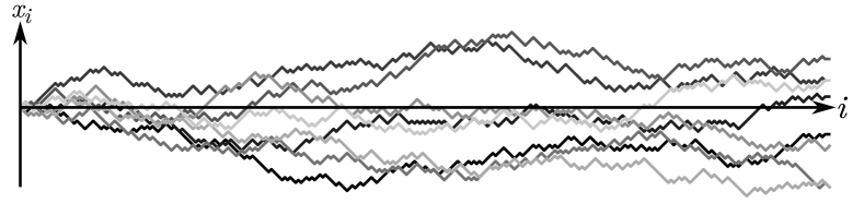
Figure 1: A number of $8$ independent symmetric $1D$ random walks, where each walk takes a number of $N=300$ steps. The position after the $i$th step (horizontal axis) is referred to as $x_{i}$ (vertical axis). The individual line segments connect subsequent positions along the $1D$ random walk.

 

Example: The symmetric $1D$ random walk

The $1D$ random walk, see Fig. 1, is a very basic example of a trajectory that evolves along the line of integer numbers $\mathbb{Z}$. Let us agree that each step along the walk has length $1$, leading to the left or right with equal probability (such a walk is referred to as symmetric).

Now, consider a random experiment that reads: Take a step! Then, the sample space which specifies the set of all elementary events for the random experiment is just $\Omega=\{\text{left},\text{right}\}$. To signify the effect of taking a step we might use a random variable $X$ that results in $X(\text{left})=-1$ and $X(\text{right})=1$. Note that this is an example of a discrete random variable.

Further, let us consider a symmetric $1D$ random walk that starts at the distinguished point $x_{0}=0$ and takes $N$ successive steps, where the position after the $i$th step is $x_{i}$.

As random experiment one might ask for the end position of the walk after $N$ successive steps. Thus, the random experiment reads: Determine the end position $x_{N}$ for a symmetric $1D$ random walk, attained after $N$ independent steps! In order to accomplish this, we might refer to the same random variable as above, where $\Omega=\{\text{left},\text{right}\}$, $X(\text{left})=-1$, and $X(\text{right})=1$. A proper random variable that tells the end position of the walk after an overall number of $N$ steps is simply $Y=\sum_{i=0}^{N-1}X^{(i)}$. The numerical value of the end position is given by $x_{N}=\sum_{i=0}^{N-1}X(\omega_{i})$, wherein $\omega_{i}$ signifies the outcome of the $i$th random experiment (i.e. step).

 

The behavior of such a random variable is fully captured by the probabilities of observing outcomes smaller or equal to a given value $x$. To put the following arguments on solid ground, we need the concept of a probability function

$$P:2^{\Omega}\rightarrow[0,1]\qquad\Big{(}\text{\parbox{130.08731pt}{$P=$ probability function $2^{\Omega}=$ power set}}\Big{)},$$ (3)

wherein $2^{\Omega}$ specifies the set of all subsets of the sample space $\Omega$ (also referred to as power set). In general, the probability function satisfies $P(\Omega)=1$ and for two disjoint events $A^{(1)}$ and $A^{(2)}$ one has $P(A^{(1)}\cup A^{(2)})=P(A^{(1)})+P(A^{(2)})$. Further, if one performs a random experiment twice, and if the experiments are performed independently, the total probability of a particular event for the combined experiment is the product of the single-experiment probabilities. I.e., for two events $A^{(1),(2)}$ one has $P(A^{(1)},A^{(2)})=P(A^{(1)})P(A^{(2)})$.

 

Example: Probability function

For the sample space $\Omega=\{\text{left},\text{right}\}$, associated to the random variable $X$ considered in the above example on the symmetric $1D$ random walk, one has the power set $2^{\Omega}=\{\emptyset,\{\text{left}\},\{\text{right}\},\{\text{left},\text{right}\}\}$. Consequently, the probability function reads: $P(\emptyset)=0$, $P(\{\text{left}\})=P(\{\text{right}\})=0.5$, and $P(\{\text{left},\text{right}\})=1$. Further, if two successive steps of the symmetric $1D$ random walk are considered, the probability for the (exemplary) combined outcome $(\text{left},\text{left})$ reads: $P(\{(\text{left},\text{left})\})=P(\{\text{left}\})P(\{\text{left}\})=0.25$.

 

By means of the probability function $P$, the (cumulative) distribution function $F_{X}$ of a random variable $X$ signifies a function

$$F_{X}:\mathbb{R}\rightarrow[0,1],~{}\text{where}~{}F_{X}=P(X\leq x)\qquad\Big{(}\text{\parbox{151.76964pt}{$F_{X}=$ distribution function $P=$ probability function}}\Big{)}.$$ (4)

The distribution is non-decreasing, implying that $F_{X}(x_{1})\leq F_{X}(x_{2})$ for $x_{1}<x_{2}$, and normalized, i.e., $\lim_{x\to-\infty}F_{X}(x)\to 0$ and $\lim_{x\to\infty}F_{X}(x)\to 1$. Further, it holds that $P(x_{0}<X\leq x_{1})=F_{X}(x_{1})-F_{X}(x_{0})$.

Considering the result of a sequence of random experiments, it is useful to draw a distinction between different types of data, to be able to choose a proper set of methods and tools for post-processing. Subsequently, we will distinguish between discrete random variables (as, e.g., the $1D$ random walk used in the above examples) and continuous random variables.

Discrete probability distributions

Besides the concept of the distribution function, an alternative description of a discrete random variable $X$ is possible by means of its associated probability mass function (pmf),

$$p_{X}:\mathbb{R}\rightarrow[0,1],~{}\text{where}~{}p_{X}(x)=P(X=x)\qquad\Big{(}\text{\parbox{151.76964pt}{$p_{X}=$ prob. mass function $P=$ probability function}}\Big{)}.$$ (5)

Related to this, note that a discrete random variable can only yield a countable number of outcomes (for an elementary step with unit step length in the $1D$ random walk problem these where just $\pm 1$) and hence, the pmf is zero almost everywhere. E.g., the nonzero entries of the pmf related to the random variable $X$ considered in the context of the symmetric $1D$ random walk are $p_{X}(-1)=p_{X}(1)=0.5$. Finally, the distribution function is related to the pmf via $F_{X}(x)=\sum_{\tilde{x}_{i}\leq x}p_{X}(\tilde{x}_{i})$ (where $\tilde{x}_{i}$ refers to those outcomes $u$ for which $p_{X}(u)>0$).

Figure 2: Results for the symmetric $1D$ random walk. (a) approximate pmf associated to the end positions after $N=100$ steps (solid vertical lines) for the symmetric $1D$ random walk as compared to a Gaussian distribution with zero mean and width $\sqrt{N}$ (dashed curve), and (b) related distribution function. For the figure, a number of $n=10^{5}$ independent random walks where considered.

 

Example: Monte Carlo simulation for the symmetric $1D$ random walk

Let us fix the number of steps in an individual symmetric $1D$ random walk to $N=100$ and consider an ensemble of $n=10^{5}$ independent walks. Now, what does the distribution of end points $x_{N}$ of the ensemble of walks thus considered look like?

If you want to tackle that question by means of computer simulations, you may follow the subsequent three steps:

(i) Implement the symmetric $1D$ random walk model using your favorite programming language. Using $\tt{python}$ [4], a minimal program to simulate the above model (1D_randWalk.py, see supplementary material) reads:

1 from random import seed, choice2 N = 1003 n = 1000004 for s in range(n):5   seed(s)6   endPos = 0 7   for i in range(N):8      endPos += choice([-1,1])9   print s,endPos In line 1, the convenient random module that implements pseudo-random number generators (PRNGs) for different distributions is imported. The function seed() is used to set an initial state for the PRNG, and choice() returns an element (chosen uniformly at random) from a specified list. In lines 2 and 3, the number of steps in a single walk and the overall number of independent walks are specified, respectively. In lines 6–7, a single path is constructed and the seed as well as the resulting final position are sent to the standard outstream in line 9. It is a bit tempting to include data post-processing directly within the simulation code above. However, from a point of view of data analysis you are more flexible if you store the output of the simulation in an external file. Then it is more easy to “revisit” the data, in case you want to (or are asked to) perform some further analyses. Hence, we might invoke the python script on the command line and redirect its output as follows

1 > python 1D_randWalk.py > N100_n100000.datAfter the script has terminated successfully, the file N100_n100000.dat keeps the simulated data available for post-processing at any time.

(ii) An approximate pmf associated to the distribution of end points can be constructed from the raw data contained in file N100_n100000.dat. We might write a small, stand-alone python script that handles that issue. However, from a point of view of code-recycling and modularization it is more rewarding to collect all “useful” functions, i.e., functions that might be used again in a different context, in a particular file that serves as some kind of tiny library. If we need a data post-processing script, we can then easily include the library file and use the functions defined therein. As a further benefit, the final data analysis scripts will consist of a few lines only. Here, let us adopt the name MCS2012_lib.py (see supplementary material) for the tiny library file and define two functions as listed below:

1  def fetchData(fName,col=0,dType=int): 2  myList = [] 3  file = open(fName,"r") 4  for line in file: 5  myList.append(dType(line.split()[col])) 6  file.close() 7  return myList 8 9  def getPmf(myList): 10  pMap = {} 11  nInv = 1./len(myList) 12  for element in myList: 13     if element not in pMap: 14        pMap[element] = 0. 15    pMap[element] += nInv 16 return pMap

Lines 1–7 implement the function fetchData(fName,col=0,dType=int), used to collect data of type dType from column number col (default column is 0 and default data type is int) from the file named fName. In function getPmf(myList), defined in lines 9–16, the integer numbers (stored in the list myList) are used to approximate the underlying pmf.

So far, we started to build the tiny library. A small data post-processing script (pmf.py, see supplementary material) that uses the library in order to construct the pmf from the simulated data reads:

1  import sys 2  from MCS2012_lib import * 3 4  ## parse command line arguments 5  fileName = sys.argv[1] 6  col      = int(sys.argv[2]) 7 8  ## construct approximate pmf from data 9  rawData  = fetchData(fileName,col) 10  pmf      = getPmf(rawData) 11 12  ## dump pmf/distrib func. to standard outstream 13  FX = 0. 14  for endpos in sorted(pmf): 15 FX += pmf[endpos] 16 print endpos,pmf[endpos],FX

This already illustrates lots of the python functionality that is needed for a decent data post-processing. In line 1, a basic python module, called sys, is imported. Among other things, it allows to access command line parameters stored as a list with the default name sys.argv. Note that the first entry of the list is reserved for the file name. All “real” command line parameters start at the list index 1. In line 2, all functions contained in the tiny library MCS2012_lib.py are imported and are available for data post-processing by means of their genuine name (no MCS2012_lib. statement has to precede a functions name). In lines 14–16, the approximate pmf as well as the related distribution function are sent to the standard outstream (for a comment on the built-in function sorted(), see paragraph “Basic sorting” in Section 1).

To cut a long story short, the approximate pmf for the end positions of the symmetric $1D$ random walks stored in the file N100_n100000.dat can be obtained by calling the script on the command line via

1 > python pmf.py N100_n100000.dat 1 > N100_n100000.pmfTherein, the digit $1$ indicates the column of the supplied file where the end position of the walks is stored, and the approximate pmf and the related distribution function are redirected to the file N100_n100000.pmf.

(iii) On the basis of analytical theory, one can expect that the enclosing curve of the pmf is well represented by a Gaussian distribution with mean $0$ and width $\sqrt{N}$. However, we need to rescale the approximate pmf, i.e., the observed probabilities, by a factor of $2$ if we want to compare it to the expected probabilities given by the Gaussian distribution. Therein, the factor $2$ reflects the fact that if we consider walks with an even (or odd) number of steps only, the effective length-scale that characterizes the distance between two neighboring positions is $2$. A less handwaving way to arrive at that conclusion is to start with the proper end point distribution for a symmetric $1D$ random walk, given by a (discrete) symmetric binomial distribution (see Section 2.4), and to approximate it, using Stirlings expansion, by a (continuous) distribution. The factor $2$ is then immediate. Using the convenient gnuplot plotting program [5], you can visually inspect the difference between the observed and expected probabilities by creating a file, e.g. called endpointDistrib.gp (see supplementary material), with content:

1  set multiplot 2 3  ## probability mass function 4   set origin 0.,0. 5   set size 0.5,0.65 6   set key samplen 1. 7   set yr [:0.05]; set ytics (0.00,0.02,0.04) 8   set xr [-50:50] 9   set xlabel "x_N" font "Times-Italic" 10   set ylabel "p_X(X=x_N)" font "Times-Italic" 11 12   ## expected probability 13   f(x)=exp(-(x-mu)**2/(2*s*s))/(s*sqrt(2*pi)) 14   mu=0; s=10 15 16   p "N100_n100000.pmf" u 1:($2/2) w impulses t "observed"\ 17   , f(x) t "expected" 18 19  ## distribution function 20   set origin 0.5,0. 21   set size 0.5,0.65 22   set yr [0:1]; set ytics (0.,0.25,0.5,0.75,1.) 23   set xr [-50:50] 24   set ylabel "F_X(x_N)" font "Times-Italic" 25 26   p "N100_n100000.pmf" u 1:($3) w steps notitle 27 28  unset multiplot Calling the file via gnuplot -persist endpointDistrib.gp, the output should look similar to Fig. 2.

 

Continuous probability distributions

Given a continuous distribution function $F_{X}$, the density of a continuous random variable $X$, referred to as probability density function (pdf), reads

$$p_{X}:\mathbb{R}\rightarrow[0,1],~{}\text{where}~{}p_{X}(x)=\frac{dF_{X}(x)}{dx}\qquad\Big{(}\text{\parbox{130.08731pt}{$p_{X}=$ prob. density function $F_{X}=$ distribution functin}}\Big{)}.$$ (6)

The pdf is strictly nonnegative, and, as should be clear from the definition, the probability that $X$ falls within a certain interval, say $x\to x+\Delta x$, is given by the integral of the pdf $p_{X}(x)$ over that interval, i.e. $P(x<X\leq x+\Delta x)=\int_{x}^{x+\Delta x}~{}p_{X}(u)~{}du$. Since the pdf is normalized, one further has $1=\int_{-\infty}^{\infty}p_{X}(u)~{}du$.

 

Example: The continuous $2D$ random walk

The continuous $2D$ random walk (see Fig. 3) is an example for a random walk with fixed step-length (for simplicity assume unit step length), where the direction of the consecutive steps is drawn uniformly at random. As continuous random variable $X$ we may choose the distance of the walk to its starting point after a number of $N$ steps, referred to as $R_{N}$. To implement this random walk model, we can recycle the python script for the $1D$ random walk, written earlier. A proper code (2d_randWalk.py, see supplementary material) to simulate the model is listed below:

1  from random import seed, random 2  from math import sqrt, cos, sin, pi 3 4  N = 100 5  n = 100000 6  for s in range(n): 7    seed(s) 8    x = y = 0. 9    for i in range(N): 10       phi = random()*2*pi 11       x  += cos(phi) 12       y  += sin(phi) 13    print s,sqrt(x*x+y*y)

Therein, in line 10, the direction of the upcoming step is drawn uniformly at random, and, in lines 11–12, the two independent walk coordinates are updated. Note that in line 2, the basic mathematical functions and constants are imported. Finally, in line 13, the distance $R_{N}$ for a single walk is sent to the standard output. Invoking the script on the command line and redirecting its output to the file 2dRW_N100_n100000.dat, we can further obtain an approximation to the underlying pdf by constructing a normalized histogram of the distances $R_{N}$ by means of the script hist.py (see supplementary material) as follows:

1 > python hist.py 2dRW_N100_n100000.dat 1 100 \2 > > 2dRW_N100_n100000.pdfThe two latter numbers signify the column of the file, where the relevant data is stored, and the desired number of bins, respectively. At this point, let us just use the script hist.py as a “black-box” and postpone the discussion of histograms until Section 2.2. After the script has terminated successfully, the file 2dRW_N100_n100000.pdf contains the normalized histogram. For values of $N$ large enough, one can expect that $R_{N}$ is properly characterized by the Rayleigh distribution

$$p_{N}(R_{N})=\frac{R_{N}}{\sigma^{2}}\exp\{-R_{N}^{2}/(2\sigma^{2})\}~{},$$ (7)

where $\sigma^{2}=(2n)^{-1}\sum_{i=0}^{n-1}R_{N,i}^{2}$. Therein, the values $R_{N,i}$, $i=0\ldots n-1$, comprise the sample of observed distances. In order to compute $\sigma$ for the sample of observed distances, one could use a cryptic python one-liner. However, it is more readable to accomplish that task in the following way (sigmaRay.py, see supplementary material):

1 import sys,math2 from MCS2012_lib import fetchData34 rawData = fetchData(sys.argv[1],1,float)56 sum2=0.7 for val in rawData: sum2+=val*val8 print "sigma=",math.sqrt(sum2/(2.*len(rawData))) Invoking the script on the command line yields:

1 > python sigmaRay.py 2dRW_N100_n100000.dat2 sigma= 7.09139394259Finally, an approximate pdf of the distance to the starting point of the walkers, i.e., a histogram using 100 bins, as well as the Rayleigh probability distribution function with $\sigma=7.091$ is shown in Fig. 3(b).

 

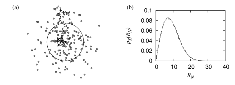
Figure 3: Results for the $2D$ random walk. (a) Snapshot of an ensemble of $n=150$ independent walkers (grey dots) after $N=200$ steps. The trail of a single walker is indicated by the zigzag line. The origin of that line also indicates the common starting point of all walkers. Further, the circle denotes the average distance $\langle R_{N}\rangle$ of the walks to the starting point after $N=200$ steps. (b) Approximate pdf for the distance to the starting point (using $100$ bins indicated by the solid step-curve, see Section 2.2 on histograms below), estimated from $n=10^{5}$ walks after $N=100$ steps, compared to the functional form (dashed line) explained in the text.

Basic parameters related to random variables

To characterize the gross features of a distribution function, it is useful to consider statistical measures that are related to its moments. Again, drawing a distinction between discrete and continuous random variables, the $k$th moment of the distribution function, related to some random variable $X$, reads

$$E[X^{k}]=\begin{cases}\sum_{i}x_{i}^{k}~{}p_{X}(x_{i}),&\text{for $X$ \emph{discrete}, and $p_{X}=$ pmf,}\\ \int_{-\infty}^{\infty}x^{k}~{}p_{X}(x)~{}dx,&\text{for $X$ \emph{continuous}, and $p_{X}=$ pdf.}\end{cases}$$ (8)

Therein, $E[\cdot]$ denotes the expectation operator.

Usually, numerical simulations result in a large but finite amount of data and the random variables considered therein yield a sequence of effectively discrete numerical values. As a consequence, from a practical point of view, the pdf underlying the data is not known precisely. Bearing this in mind, we proceed by estimating the gross statistical features of a sample of $N$ statistically independent numerical values $x=\{x_{0},\ldots,x_{N-1}\}$, i.e., the associated random variables are assumed to be independent and identically distributed. For simplicity, we may assume the uniform pmf $p_{X}(x_{i})=1/N$ for $i=0\ldots N-1$. Commonly, $N$ is referred to as sample size. The average or mean value of the sample is then properly estimated by the finite sum

$${\rm av}(x)=\frac{1}{N}\sum_{i=0}^{N-1}x_{i}~{},\qquad\text{(average or mean value)},$$ (9)

which simply equates the finite sequence to the first moment of the (effectively unknown) underlying distribution. Note that for values that stem from a probability distribution that decreases slowly as $x\to\infty$ (aka having a broad tail), the convergence properties of the sum might turn out to be very poor for increasing $N$. Further, one might be interested in the spread of the values within the sample. A convenient measure related to that is the variance, defined by

$${\rm Var}(x)=\frac{1}{N-1}\sum_{i=0}^{N-1}[x_{i}-{\rm av}(x)]^{2}~{}.\qquad\text{(variance)}.$$ (10)

Essentially, the variance measures the mean squared deviation of the values contained in the sequence, relative to the mean value. Usually, the mean is not known a priori and has to be estimated from the data beforehand, e.g. by using Eq. (9). This reduces the number of independent terms of the sum by one and leads to the prefactor of $N-1$. To be more precise, Eq. (10) defines the corrected variance, as opposed to the uncorrected variance ${\rm uVar}(x)=(N-1)/N\times{\rm Var}(x)$. The latter one can also be written as ${\rm uVar}(x)={\rm av}([x-{\rm av}(x)]^{2})$. While the corrected variance is an unbiased estimator for the spread of the values within the sequence, the uncorrected variance is biased (see discussion below). A note on implementation: in order to improve on a naive implementation, and so to reduce the round-off error in Eq. (10), the so-called “corrected two-pass algorithm” (see Ref. [20]) might be used. The square root of the variance yields the standard deviation

$${\rm sDev}(x)=\sqrt{{\rm Var}(x)}~{}.\qquad\text{(standard deviation)}$$ (11)

At this point, note that the variance and standard deviation depend on the second moment of the underlying distribution. Again, the subtleties of an underlying distribution with a broad tail might lead to a non-converging variance or standard deviation as $N\to\infty$ (see example below). For a finite sequence of values, the standard error of the mean, referred to as sErr, is also a measure of great treasure. Assuming that the values in the sample are statistically independent, it is related to the standard deviation by means of

$${\rm sErr}(x)=\frac{{\rm sDev}(x)}{\sqrt{N}}~{}.\qquad\text{(standard error).}$$ (12)

For a finite sample size $N$, the standard error is of interest since it gives an idea of how accurate the sample mean approximates the true mean (attained in the limit $N\to\infty$).

 

Example: Basic statistics

We may amend the tiny library MCS2012_lib.py by implementing the function basicStatistics() as listed below:

1  def basicStatistics(myList): 2 av = var = tiny = 0. 3 N = len(myList) 4 for el in myList: 5 av += el 6 av /= N 7 for el in myList: 8 dum   = el - av 9 tiny += dum 10 var  += dum*dum 11 var  = (var - tiny*tiny/N)/(N-1) 12 sDev = sqrt(var) 13 sErr = sDev/sqrt(N) 14 return av, sDev, sErr Therein, the variance of the numerical values contained in the list myList is computed by means of the corrected two-pass algorithm. To facilitate the computation of the standard deviation, we further need to import the square root function, available in the math module, by adding the line from math import sqrt at the very beginning of the file.

Good convergence (Gaussian distributed data):

In a preceding example we gained the intuition that the pmf of the end points for a symmetric $1D$ random walk, involving a number of $N$ steps, can be expected to compare well to a Gaussian distribution with mean $\langle x_{N}\rangle=0$ ($={\tt av}(x)$ as $n\to\infty$; $n=$sample size) and width $\sigma=\sqrt{N}$ ($={\tt sDev}(x)$ as $n\to\infty$). In order to compute averages of data stored in some file, we may write a small data analysis script (basicStats.py, see supplementary material) as listed below:

1  import sys 2  from MCS2012_lib import * 3 4  ## parse command line arguments 5  fileName     = sys.argv[1] 6  col          = int(sys.argv[2]) 7 8  ## construct approximate pmf from data 9  rawData      = fetchData(fileName,col) 10  av,sDev,sErr = basicStatistics(rawData) 11 12  print "av   = %4.3lf"%av 13  print "sErr = %4.3lf"%sErr 14  print "sDev = %4.3lf"%sDev Basically, the script imports all the functions defined in the tiny library MCS2012_lib.py (line 2), reads the data stored in a particular column of a supplied file (line 9) and computes the mean, standard deviation and error associated to the sequence of numerical values (line 10). If we invoke the script for the data accumulated for the symmetric $1D$ random walk (bear in mind to indicate the column number where the data can be found), it yields:

1 > python basicStats.py N100_n100000.dat 12 av   = 0.0083 sErr = 0.0324 sDev = 10.022Apparently, the results of the Monte Carlo simulation are in agreement with the expectation.

Poor convergence (power-law distributed data):

The probability density function $p_{X}(x)$ for power-law distributed continuous real variables $x$ can be written as

$$p_{X}(x)=\frac{\alpha-1}{x_{0}}\Big{(}\frac{x}{x_{0}}\Big{)}^{-\alpha}\sim x^{-\alpha},\qquad\text{(power-law pdf),}$$ (13)

where, in order for the pdf to be normalizable, we might assume $\alpha>1$, and where $x_{0}$ shall denote the smallest $x$-value for which the power-law behavior holds. Pseudo random numbers, drawn according to this pdf, can be obtained via the inversion method. For that, one draws a random real number $r$ uniformly in $[0,1)$ and generates a power-law distributed random number $x$ as $x=x_{0}(1-r)^{-1/(\alpha-1)}$, where $x_{0}\leq x<\infty$. A small, stand-alone python script (poorConvergence.py; see supplementary material) that implements the inversion method to obtain a sequence of $N=10^{5}$ random real numbers drawn from the power-law pdf with $\alpha=2.2$ and $x_{0}=1$ is listed below:

1  from random import seed, random 2  from MCS2012_lib import basicStatistics 3 4  ## inversion method to obtain power law 5  ## distributed pseudo random numbers 6  N = 100000 7  seed(0) 8  alpha = 2.2 9  myList = [] 10  for i in range(N): 11 r = pow(1.-random() , -1./(alpha-1.)  ) 12 myList.append(r) 13 14  ## basic statistics for different sample sizes to 15  ## assess convergence properties for av and sDev 16  M = 100; dN = N/M 17  for Nmax in [dN+i*dN for i in range(M)]: 18 av,sDev,sErr = basicStatistics(myList[:Nmax]) 19 print Nmax, av, sErr, sDev In line 2, the function basicStatistics(), as defined in MCS2012_lib.py, is imported and available for data post-processing. The inversion method to obtain random numbers according to Eq. (13) is implemented in lines 10 and 11. The resulting numbers are stored in a list which is subsequently used to estimate the mean, standard error of the mean and standard deviation for a number of $N=10^{3}\ldots 10^{5}$ (in steps of $\Delta N=1000$) samples (lines 16–19). As a result, the convergence properties of the mean and standard error are shown in Fig. 4. Apparently, the estimate for the mean converges quite well (see Fig. 4(a)), while the standard deviation exhibits poor convergence properties (see main plot of Fig. 4(b)). In such a case, the standard deviation is said to be not robust. On second thought, this is intuitive, since for the moments of a power-law distribution it holds that

$$\langle x^{k}\rangle=\frac{\alpha-1}{x_{0}^{-\alpha+1}}\int_{x_{0}}^{\infty}x^{-\alpha+k}~{}dx=\frac{\alpha-1}{x_{0}^{-\alpha+1}}\Big{[}\frac{x^{-\alpha+k+1}}{(-\alpha+k+1)}\Big{]}_{x_{0}}^{\infty}~{},$$ (14)

and thus one arrives at the conclusion that $\langle x^{k}\rangle$ is finite only if $k+1<\alpha$ while all higher moments diverge. In particular, for $\alpha=2.2$, the second moment of the distribution, needed to compute the variance, does not converge as the sample size increases. Note that a more robust estimate of the deviations within the data set is provided by the absolute deviation

$${\rm aDev}(x)=\frac{1}{N}\sum_{i=0}^{N-1}|x_{i}-{\rm av}(x)|~{},\qquad\text{(absolute deviation),}$$ (15)

shown in the inset of Fig. 4(b).

 

Figure 4: Results for estimating (a) the mean (error bars denote the standard error), and (b) the standard deviation, for a sequence of $N=10^{3}\ldots 10^{5}$ random numbers (in steps of $\Delta N=1000$) drawn from a power-law pdf with $\alpha=2.2$ and $x_{0}=1$. Apparently, the mean converges well and the standard deviation exhibits rather poor convergence properties. However, the absolute deviation shown in the inset of (b) represents a more robust estimation of the deviation within the data set.

Estimators with(out) bias

In principle, there is no strict definition of how to ultimately estimate a specific parameter $\phi$ for a given data set $x$. To obtain an estimate for $\phi$, an estimator (for convenience let us refer to it as $\hat{\phi}(x)$) is used. The hope is that the estimator maps a given data set to a particular value that is close to $\phi$. However, regarding a specific parameter, it appears that some estimators are better suited than others. In this regard, a general distinction is drawn between biased and unbiased estimators. To cut a long story short, an estimator is said to be unbiased if it holds that $E[\hat{\phi}(x)]=\phi$. Therein, the computation of the expected value is with respect to all possible data sets $x$. In words: an estimator is unbiased if its expectation value is equal to the true value of the parameter. Otherwise, $\hat{\phi}$ is biased.

To be more specific, consider a finite set of $N$ numerical values $x=\{x_{0},\ldots,x_{N-1}\}$, where the associated random variables are assumed to be independent and identically distributed, following a pdf with (true) mean value $\mu$ and (true) variance $\sigma^{2}$. As an example for an unbiased estimator, consider the computation of the mean value, i.e. $\phi\equiv\mu$. As an estimator we might use the definition of the sample mean according to Eq. (9), i.e. $\hat{\phi}(x)\equiv{\rm av}(x)$. We thus have

$$E[{\rm av}(x)]=\frac{1}{N}\sum_{i=0}^{N-1}E[x_{i}]=\frac{1}{N}(N\mu)=\mu~{}.$$ (16)

Further, the mean square error (MSE) $E[(\hat{\phi}(x)-\phi)^{2}]$ of the estimator ${\rm av}(x)$ reads

$$E[({\rm av}(x)-\mu)^{2}]=\frac{1}{N^{2}}\sum_{i=0}^{N-1}E[(x_{i}-\mu)^{2}]=\frac{1}{N^{2}}(N\sigma^{2})=\frac{\sigma^{2}}{N}~{}.$$ (17)

In principle, the MSE measures both, the variance of an estimator and its bias. Consequently, for an unbiased estimator as, e.g., the definition of the sample mean used above, the MSE is equal to its variance. Further, since $\lim_{N\to\infty}E[({\rm av}(x)-\mu)^{2}]=0$, the estimator is said to be consistent.

As an example for a biased estimator, consider the computation of the variance, i.e. $\phi\equiv\sigma^{2}$. As an estimator we might use the uncorrected variance, as defined above, to find

$$E[{\rm uVar}(x)]=\frac{1}{N}\sum_{i=0}^{N-1}E[(x_{i}-\mu)^{2}]-E[({\rm av}(x)-\mu)^{2}]=\frac{N-1}{N}\sigma^{2}~{}.$$ (18)

Since here it holds that $E[{\rm uVar}(x)]\neq\sigma^{2}$, the uncorrected variance is biased. Note that the (corrected) variance, defined in Eq. (10), provides an unbiased estimate of $\sigma^{2}$. Finally, note that the question whether bias arises is solely related to the estimator, not the estimate (obtained from a particular data set).

2.2 Histograms: binning and graphical representation of data

In the preceding section, we have already used histograms as a tool to construct approximate distribution functions from a finite set of data. Now, to provide a more precise definition of a histogram, consider a data set $x\equiv\{x_{i}\}_{i=0}^{N-1}$ that stems from repeated measurements of a continuous random variable $X$ during a random experiment. To get a gross idea of the properties of the underlying continuous distribution function, and to allow for a graphical representation of the respective data, e.g., for the purpose of communicating results to the scientific community, a histogram of the observed data is of great use.

The idea is simply to accumulate the elements of the data set $x$ in a finite number of, say, $n$ distinct intervals (or classes) $C_{i}=[c_{i},c_{i+1})$, $i=0\ldots n-1$, called bins, where the $c_{i}$ specify the interval boundaries. The frequency density $h_{i}$ (i.e., the relative frequency per unit-interval) associated with the $i$th bin can easily be obtained as $h_{i}=n_{i}/(N\Delta c_{i})$, where $n_{i}$ specifies the number of elements that fall into bin $C_{i}$, and $\Delta c_{i}=c_{i+1}-c_{i}$ is the respective bin width. The resulting set $H$ of tuples $(C_{i},h_{i})$, i.e.

$$H=\{(C_{i},h_{i})\}_{i=0}^{n-1}~{},\qquad\Big{(}\text{\parbox{164.77771pt}{$C_{i}=[c_{i},c_{i+1})$, i.e.\ the $i$th bin $h_{i}=$ frequency density}}\Big{)},$$ (19)

specifies the histogram and give a discrete approximation to the pdf underlying the random variable. Note that if one considers a finite sample size $N$, it is only possible to construct an approximate pdf. However, as the sample size increases one can be confident to approximate the true pdf quite well. All the values that fall within a certain bin $C_{i}$ are further represented by a particular value $x_{i}^{\prime}\in C_{i}$. Often, $x_{i}^{\prime}$ is chosen as the center of the bin. Also note that, in order to properly represent the observed data, it might be useful to choose different widths $\Delta c_{i}=c_{i+1}-c_{i}$ for the different bins $b_{i}$. As an example, one may decide to go for linear or logarithmic binning, detailed below.

Linear binning

Considering linear binning, the whole range of data $[x_{\rm min},x_{\rm max})$ is collected using $n$ bins of equal width $\Delta c=(x_{\rm max}-x_{\rm min})/n$. Therein, a particular bin $C_{i}$ accumulates all elements in the interval $[c_{i},c_{i+1})$, where the interval bounds are given by

$$c_{i}=x_{\rm min}+i\Delta c~{},~{}{\text{for}}~{}i=0\ldots n~{}.$$ (20)

During the binning procedure, a particular element belongs to bin $C_{i}$, where the integer identifier of the bin is given by $i=\lfloor x/\Delta c\rfloor$.

Logarithmic binning

Considering logarithmic binning, the whole range of data $[x_{\rm min},x_{\rm max})$ is collected within $n$ bins that have equal width on a logarithmic scale, i.e., $\log(c_{i+1})=\log(c_{i})+\Delta c^{\prime}$ where $\Delta c^{\prime}=\log(x_{\rm max}/x_{\rm min})/n$. In case of logarithmic binning, a particular bin $C_{i}$ accumulates all elements in the interval $[c_{i},c_{i+1})$, where the interval bounds are consequently given by

$$c_{i}=c_{0}\times\exp\{i\Delta c^{\prime}\}~{},~{}{\text{for}}~{}i=0\ldots n~{}.$$ (21)

During the histogram build-up, a particular element belongs to bin $C_{i}$, where $i=\lfloor\log(x/x_{\rm min})/\Delta c^{\prime}\rfloor$. Note that on a linear scale, the width of the bins increases exponentially, i.e. $\Delta c_{i}=c_{i}\times(\exp\{\Delta c^{\prime}\}-1)\propto c_{i}$. Such a binning is especially well suited to represent power-law distributed data, see the example below.

A general drawback of any binning procedure is that many data in a given range $[c_{i},c_{i+1})$ are represented by only a single representative $x_{i}^{\prime}$ of that interval. As a consequence, data binning always comes to the expense of information loss.

 

Example: Data binning

A small code-snippet that illustrates a python implementation of a histogram using linear binning is listed below as hist_linBinning():

1  def hist_linBinning(rawData,xMin,xMax,nBins=10): 2 h = [0]*nBins 3 4 dx = (xMax-xMin)/nBins 5 def binId(val):   return int(floor((val-xMin)/dx)) 6 def bdry(i):      return xMin+i*dx, xMin+(i+1)*dx 7 def GErr(q,n,dx): return sqrt(q*(1-q)/(N-1))/dx 8 9 for value in rawData: 10    if 0 <= binId(value) < nBins: 11       h[binId(value)] += 1 12 13 N = sum(h) 14 for bin in range(nBins): 15    hRel   = float(h[bin])/N 16    low,up = bdry(bin) 17    width  = up-low 18    print low, up, hRel/width, GErr(hRel,N,width) The first argument in the function call, see line 1 of the code listing, indicates a list of the raw data, followed by the minimal and maximal variable value that should be considered during the binning procedure. The last argument in the function call specifies the number of bins that shall be used therein (the default value is set to 10). Based on the supplied data range and number of bins, the uniform bin width is computed in line 4. Note that within the function hist_linBinning(), 3 more functions are defined. Those facilitate the calculation of the integer bin id that corresponds to an element of the raw data (line 5), the lower and upper boundaries of a bin (line 6), and the Gaussian error bar for the respective data point (line 7). In lines 9–11, the binning procedure is kicked off. Since the upper bin boundary is exclusive, bear in mind that the numerical value xMax is identified with the bin index nBins+1. As a consequence it will not be considered during the histogram build-up. Finally, in lines 13–18 the resulting normalized bin entries and their associated errors are sent to the standard out-stream. The function is written in a quite general form, so that in order to implement a different kind of binning procedure only the definitions in lines 4–7 have to be modified. As regards this, for a more versatile variant that offers linear or logarithmic binning of the data, see the function hist in the tiny library MCS2012_lib.py.

Binning of the data obtained for the $2D$ random walk:

The approximate pdf of the average distance to the starting point for $10^{5}$ independent $100$-step $2D$ random walks, see Fig. 3, was obtained by a linear binning procedure using the function hist_linBinning() outlined above. For that task, the small script hist.py listed below (see supplementary material) was used:

1 import sys2 from MCS2012_lib import fetchData, hist_linBinning34 fName = sys.argv[1]5 col   = int(sys.argv[2])6 nBins = int(sys.argv[3])7 myData = fetchData(fName,col,float)8 hist_linBinning(myData,min(myData),max(myData),nBins) In principle, the Gaussian error bars are adequate for that data. However, for a clearer presentation of the results, the error bars are not shown in Fig. 3(b).

Binning of power-law distributed data:

To illustrate the pros and cons of the binning types introduced above, consider a data set consisting of $N=10^{6}$ random numbers drawn from the power-law pdf, Eq. (13), with $\alpha=2.5$ and $x_{0}=1$. Fig. 5(a) shows a histogram of the data using linear binning. In order to cover the whole range of data, the histogram uses $n=2\times 10^{4}$ bins with equal bin width $\Delta c\approx 0.36$. In principle, for a finite set of data and for power-law exponents $\alpha>1$, the number of samples per bin decreases as the bin-index $i$, see Eq. (20), increases. For a more elaborate discussion of the latter issue you might also want to consult Ref. [19]. Consequently, the tail of the (binned) distribution is rather noisy. Thus, as evident from Fig. 5(a), a linear binning procedure appears to be inadequate for power-law distributed data. One can do better by means of logarithmic binning, see Fig. 5(b). Considering log-binning, the bins in the tail accumulate more samples, resulting in reduced statistical noise. In comparison to linear binning, data points in the tail are less scattered and the power law decay of the data can be followed further to smaller probabilities. As a further benefit, on a logarithmic scale one has bins with equal width. As a drawback note that any binning procedure involves a loss of information. Also note that for the case of logarithmic binning, the Gaussian error bars are not adequate.

 

Figure 5: The plots illustrate a data set consisting of $10^{6}$ random numbers, drawn from the power-law distribution, see Eq. (13), with $\alpha=2.5$ and $x_{0}=1$. To give a visual account of the underlying probability distribution, the data was binned to yield (a) a histogram using linear binning (displayed on log scale) and an overall number of $n=2\times 10^{4}$ bins, and, (b) a histogram using logarithmic binning and $n=55$ bins (for the same data as in (a)). In either histogram, the center of a bin (on a linear scale) was chosen to represent all values that fall within that bin.

2.3 Bootstrap resampling: the unbiased way to estimate errors

In a previous section, we discussed different parameters that may serve to characterize the statistical properties of a finite set of data. Amongst others, we discussed estimators for the sample mean and standard deviation. While there was a straight forward estimator for the standard error of the sample mean, there was no such measure for the standard deviation. As a remedy, the current section illustrates a method that proves to be highly valuable when it comes to the issue of estimating errors related to quite a lot of observables (for some more details you might want to consult chapter $15.6$ of Ref. [20]), in an unbiased way. To get an idea about the subtleties of the method, picture the following situation: you perform a sequence of random experiments for a given model system and generate a sample $x$, consisting of $N$ statistically independent numbers.

Your aim is to measure some quantity $q$, e.g. some function $q\equiv f(x)$, that characterizes the simulated data. At this point, bear in mind that this does not yield the true quantity $q^{\star}$ that characterizes the model under consideration. Instead, the numerical value of $q$ (very likely) differs from the latter value to some extent. To provide an error estimate that quantifies how good the observed value $q$ approximates the true value $q^{\star}$, the bootstrap method utilizes a Monte Carlo simulation. This can be decomposed into the following two-step procedure: Given a data set $x$ that consists of $N$ numerical values, where the corresponding random variables are assumed to be independent and identically distributed:

• generate a number of $M$ auxiliary bootstrap data sets $\tilde{x}^{(k)}$, $k=0\ldots M-1$ by means of a resampling procedure. To obtain one such data set, draw $N$ data points (with replacement) from the original set $x$. During the construction procedure of a particular data set, some of the elements contained in $x$ will be chosen multiple times, while others won’t appear at all;

• measure the observable of interest for each auxiliary data set, to yield the set of estimates $\tilde{q}=\{\tilde{q}_{k}\}_{k=0}^{M-1}$. Estimate the value of the desired observable using the original data set and compute the corresponding error as the standard deviation

  $${\rm sDev}(\tilde{q})=\Big{(}\frac{1}{M-1}\sum_{k=0}^{M-1}[\tilde{q}_{k}-{\rm av}(\tilde{q})]^{2}\Big{)}^{1/2}\qquad\text{(bootstrap error estimate)}$$ (22)

  of the $M$ resampled (auxiliary) bootstrap data sets.

The finite sample $x$ only allows to get a coarse-grained glimpse on the probability distribution underlying the data. In principle, the latter one is not known. Now, the basic assumption on which the bootstrap method relies is that the values $\tilde{q}_{k}$ (as obtained from the auxiliary data sets $\tilde{x}^{(k)}$) are distributed around the value $q$ (obtained from $x$) in a way similar to how further estimates of the observable obtained from further independent simulations are distributed around $q^{\star}$. From a practical point of view, the procedure outlined above works quite well.

 

Example: Error estimation via bootstrap resampling

The code snippet below lists a python implementation of the bootstrap method outlined above. It is most convenient to amend the tiny library by the function bootstrap(). Note that it makes reference to basicStatistics(), already defined in MCS2012_lib.py.

1  def bootstrap(myData,estimFunc,M=128): 2         N        = len(myData) 3         h        = [0.0]*M 4         bootSamp = [0.0]*N 5         for sample in range(M): 6     for val in range(N): 7        bootSamp[val] = myData[randint(0,N-1)] 8     h[sample] = estimFunc(bootSamp) 9         origEstim = estimFunc(myData) 10         resError = basicStatistics(h)[1] 11         return origEstim,resError In lines 5–8, a number of $M$ auxiliary bootstrap data sets are obtained (the default number of auxiliary data sets is set to $M=128$, see function call in line 1). In line 9, the desired quantity, implemented by the function estimFunc, is computed for the original data set. Finally, the corresponding error is found as the standard deviation of the $M$ estimates of estimFunc for the auxiliary data sets in line 10. Note that the function bootstrap() needs integer random numbers, uniformly drawn in the interval $0\ldots N-1$, in order to generate the auxiliary data sets. For this purpose the line from random import randint must be included at the beginning of the file MCS2012_lib.py.

As an example we may write the following small script that computes the mean and standard deviation, along with an error for those quantities computed using the bootstrap method, for the data accumulated earlier for the symmetric $1D$ random walk (bootstrap.py, see supplementary material).

1  import sys 2  from MCS2012_lib import * 3 4  fileName = sys.argv[1] 5  M        = int(sys.argv[2]) 6  rawData  = fetchData(fileName,1) 7 8  def mean(array): return basicStatistics(array)[0] 9  def sDev(array): return basicStatistics(array)[1] 10 11  print "# estimFunc: q +/- dq" 12  print "mean: %5.3lf +/- %4.3lf"%bootstrap(rawData,mean,M) 13  print "sDev: %5.3lf +/- %4.3lf"%bootstrap(rawData,sDev,M) Note that the statement from MCS2012_lib import * imports all functions from the indicated file and makes them available for data post-processing. Invoking the script on the command line via

1  > python bootstrap.py N100_n100000.dat 1024where the latter number specifies the desired number of bootstrap samples, the bootstrap method yields the results:

1  # estimFunc: q +/- dq 2  mean:  0.008 +/- 0.032 3  sDev: 10.022 +/- 0.022For the sample mean, the bootstrap error is in good agreement with the standard error ${\rm sErr}(x)=0.032$ estimated in the “basic statistics” example (as it should be). Regarding the bootstrap error for the standard deviation, the result is in agreement with the expectation $\sigma=10$ (for a number of $100$ steps in an individual walk). In Fig. 6, the resulting distribution of the resampled estimates for the mean value (see Fig. 6(a)) and standard error (see Fig. 6(b)) are illustrated. For comparison, if we reduce the number of bootstrap samples to $M=24$ we obtain the two bootstrap errors $0.033$ and $0.024$ for the mean and standard error, respectively.

 

Figure 6: Result of the bootstrap resampling procedure ($M=1024$ auxiliary data sets) for the data characterizing the end point distribution for the symmetric $1D$ random walk. (a) Approximate pdf (histogram using 18 bins) of the resampled average value. The non-filled square marks the mean value and the associated error bar indicates the standard error as obtained in the example on “basic statistics” in Section 2.1. (b) Approximate pdf (histogram using 18 bins) of the resampled standard deviation. The estimate of both quantities, as obtained from the original data set, is indicated by a solid vertical line, while the bootstrap error bounds are shown by dashed vertical lines.

2.4 The chi-square test: observed vs. expected

The chi-square ($\chi^{2}$) goodness-of-fit test is commonly used to check whether the approximate pdf obtained from a set of sampled data appears to be equivalent to a theoretical density function. Here, “equivalent” is meant in the sense of “the observed frequencies, as obtained from the data set, are consistent with the expected frequencies, as obtained from assuming the theoretical distribution function”. More precisely, assume that you obtained a set $\{(C_{i},n_{i})\}_{i=0}^{n-1}$ of binned data, summarizing an original data set of $N$ uncorrelated numerical values, where $C_{i}=[c_{i},c_{i+1})$ signifies the $i$th bin with boundaries $c_{i}$ and $c_{i+1}$, and $n_{i}$ is the number of observed events that fall within that bin. With reference to Section 2.2, the set of binned data is referred to as frequency histogram. Further, assume you already have a (more or less educated) guess about the expected limiting distribution function underlying the data, which we call $f(x)$ in the following. Considering this expected limiting function, the number of expected events in the $i$th bin can be estimated as

$$e_{i}=N\times\int_{c_{i}}^{c_{i+1}}f(x)~{}dx\qquad\text{(expected frequencies).}$$ (23)

To address the question whether the observed data might possibly be drawn from $f(x)$, the chi-square test compares the number of observed events in a given bin to the number of expected events in that bin by means of the expression

$$\chi^{2}=\sum_{i=0}^{n-1}\frac{(n_{i}-e_{i})^{2}}{e_{i}}\qquad\text{(chi-square test).}$$ (24)

A further quantity that is important in relation to that test is the number of degrees of freedom, termed ${\rm dof}$. Usually it is equal to the number of bins less $1$, reflecting the fact that the sum of the expected events has been re-normalized to match the sample size of the original data set, i.e. $\sum_{i}e_{i}=N$. However, if the function $f(x)$ involves additional free parameters that have to be determined from the original data in order to properly represent the expected limiting distribution function, each of these free parameters decreases the number of degrees of freedom by one. Now, the wisdom behind the chi-square test is that for $\chi^{2}\approx{\rm dof}$, one can consider the observed data as being consistent with the expected limiting distribution function. If it holds that $\chi^{2}\gg{\rm dof}$, then the discrepancy between both is significant. Besides listing the values of $\chi^{2}$ and ${\rm dof}$, a more convenient way to state the result of the chi-square test is to report the reduced chi-square, i.e. chi-square per dof, $\tilde{\chi}^{2}=\chi^{2}/{\rm dof}$. It is independent of the number of degrees of freedom and the observed data is consistent with the expected distribution function if $\tilde{\chi}^{2}\approx 1$.

For an account of more strict criteria that allow to assess the “quality” of the chi-square test and what to pay attention to if one attempts to compare two sets of binned data that summarize data sets with possibly different sample sizes, see Refs. [20, 17]. Let us leave it at that. As a final note, notice that the chi-square test cannot be used to prove that the observed data is drawn from an expected distribution function, it merely reports whether the observed data is consistent with it.

 

Example: Chi-square test

The code snippet below lists a python implementation of the chi-square test outlined above. It is most convenient to amend MCS2012_lib.py by the function definition

1 def chiSquare(obsFreq,expFreq,nConstr):2        nBins = len(obsFreq)3        chi2 = 0.04        for bin in range(nBins):5           dum   = obsFreq[bin]-expFreq[bin]6           chi2 += dum*dum/expFreq[bin]7        dof = nBins-nConstr8        return dof,chi2 A word of caution: it is a good advise to not trust a chi-square test for which some of the observed frequencies are less than, say, 4 (see Ref. [12]). For such small frequencies, the statistical noise is simply too large and the respective terms might lead to an exploding value of $\chi^{2}$. As a remedy one can merge a couple of adjacent bins to form a “super-bin” containing more than just 4 events.

For an illustrational purpose we might perform a chi-square test for the approximate pmf of the end positions of the symmetric $1D$ random walks, constructed earlier in Section 2.1. In this regard, let $\{(x_{i},n_{i})\}_{i=0}^{n-1}$ be the binned set of data, summarizing an original data set (for a discrete random variable) with sample size $M$. Therein, $n_{i}$ denotes the number of observed events that correspond to the value $x_{i}$. For the data at hand, the expected frequencies $e_{i}$ are simply proportional to the symmetric binomial distribution with variance $N/4$ (where $N$ is the number of steps in a single walk) at $x_{i}$. To be more precise, we have

$$e_{i}=M\times{\rm bin}(N,(x_{i}+N)/2)2^{-N},$$ (25)

for $i=0\ldots n-1$, wherein $N$ specifies the number of steps in a single walk and ${\rm bin}(a,b)=a!/[(a-b)!b!]$ defines the binomial coefficients. For the data on the symmetric $1D$ random walk, some of the observed frequencies in the tails of the distribution are smaller than $4$. As mentioned above, this requires the pooling of several bins in the regions of low probability density. Practically speaking, we create two super-bins that lump together all frequencies that correspond to values $x_{i}\geq R$ or $x_{i}\leq-R$, respectively. This procedure works well, since the distribution is symmetric. The following script implements this re-binning procedure and performs the chi-square test as defined above:

1  import sys 2  from math import factorial as fac 3  from MCS2012_lib import * 4  import scipy.special 5 6  fileName = sys.argv[1] 7  col      = int(sys.argv[2]) 8  R        = int(sys.argv[3]) 9 10  rawData  = fetchData(fileName,col) 11  pmf      = getPmf(rawData) 12 13  def bin(n,k): return fac(n)/(fac(n-k)*fac(k)) 14  def f(x,N):   return bin(N,(x+N)*0.5)*0.5**N 15 16  N=len(rawData) 17  oFr={}; eFr={} 18  for el in pmf: 19   if el >= R: 20         if R not in oFr: 21           oFr[R] = eFr[R] = 0 22         oFr[R] += pmf[el]*N 23         eFr[R] += f(el,100)*N 24   elif el <= -R: 25         if -R not in oFr: 26           oFr[-R] = eFr[-R] = 0 27         oFr[-R] += pmf[el]*N 28         eFr[-R] += f(el,100)*N 29   else: 30         oFr[el] = pmf[el]*N 31         eFr[el] = f(el,100)*N 32 33  o = map(lambda x: x[1], oFr.items()) 34  e = map(lambda x: x[1], eFr.items()) 35 36  dof,chi2 = chiSquare(o,e,1) 37  print "# dof=%d, chi2=%5.3lf"%(dof,chi2) 38  print "# reduced chi2=%5.3lf"%(chi2/dof) 39 40  pVal = scipy.special.gammaincc(dof*0.5,chi2*0.5) 41  print "# p=",pVal

Therein, in lines 13–14, the symmetric binomial distribution is defined, and in lines 16–31 the re-binning of the data is carried out. Finally, lines 33–34 prepare the re-binned data for the chi-sqare test (line 36). Note that the script above extends the chi-square goodness-of-fit test by also computing the so-called $p$-value for the problem at hand (line 40). The $p$-value is a standard way to assess the significance of the chi-square test, see Refs. [20, 17]. In essence, the numerical value of $p$ gives the probability that the sum of the squares of a number of ${\rm dof}$ Gaussian random variables (zero mean and unit variance) will be greater than $\chi^{2}$. To compute the $p$-value an implementation of the incomplete gamma function is needed. Unfortunately, this is not contained in a standard python package. However, the incomplete gamma function is available through the scipy-package [6], which offers an extensive selection of special functions and lots of scientific tools. Considering the $p$-value, the observed frequencies are consistent with the expected frequencies, if the numerical value of $p$ is not smaller than, say, $10^{-2}$.

If the script is called for $R=40$ it yields the result:

1  > python chiSquare.py N100_n100000.dat 1 40 2  # dof=40, chi2=38.256 3  # reduced chi2=0.956 4  # p= 0.549Hence, the pmf for the end point distribution of the symmetric $1D$ random walk appears to be consistent with the symmetric binomial distribution with mean $0$ and variance $N/4$, wherein $N$ specifies the number of steps in a single walk.

 

3 Object oriented programming in python

In addition to the built-in data types used earlier in these notes, python allows you to define your own custom data structures. In doing so, python makes it easy to follow an object oriented programming (OOP) approach. The basic idea of the OOP approach is to use objects in order to design computer programs. Therein, the term ’object’ refers to a custom data structure that has certain attributes and methods, where the latter can be understood as functions that alter the attributes of the data structure.

By following an OOP approach, the first step consists in putting the problem at hand under scrutiny and figuring out what the respective objects might be. Once this first step is accomplished one might go on and design custom data structures to represent the objects. In python this is done using the concept of classes.

In general, OOP techniques emphasize on data encapsulation, inheritance, and overloading. In less formal terms, data encapsulation means to ’hide the implementation’. I.e., the access to the attributes of the data structures is typically restricted, making them (somewhat) private. Access to the attributes is only granted for certain methods that build an interface by means of which an user can alter the attributes. The concept of data encapsulation slightly interferes with the ’everything is public’ consensus of the python community which follows the habit that even if one might be able to see the implementation one does not have to care about it. Nevertheless, python offers a kind of pseudo-encapsulation referred to as name-mangling which will be illustrated in Subsection 3.2

In OOP terms, inheritance means to ’share code among classes’. It highly encourages code recycling and easily allows to extend or specialize existing classes, thereby generating a hierarchy composed of classes and derived subclasses.

Finally, overloading means to ’redefine methods on subclass level’. This makes it possible to adapt methods to their context. Also known as polymorphism, this offers the possibility to have several definitions of the same method on different levels of the class hierarchy.

3.1 Implementing an undirected graph

An example by means of which all three OOP techniques can be illustrated is a graph data structure. For the purpose of illustration consider an undirected graph $G=(V,E)$. Therein, the graph $G$ consists of an unordered set of $n=|V|$ nodes $i\in V$ and an unordered set of $m=|E|$ edges $\{i,j\}\in E$ (cf. the contribution by Hartmann in this volume).

According to the first step in the OOP plan one might now consider the entity graph as an elementary object for which a data structure should be designed. Depending on the nature of the graph at hand there are different ’optimal’ ways to represent them. Here, let us consider sparse graphs, i.e., graphs with $O(m)\ll O(n^{2})$. In terms of memory consumption it is most beneficial to choose an adjacency list representation for such graphs, see Fig. 7(a). This only needs space $O(n+2m)$. An adjacency list representation for $G$ requires to maintain for each node $i\in V$ a list of its immediate neighbors. I.e., the adjacency list for node $i\in V$ contains node $j\in V$ only if $\{i,j\}\in E$. Hence, as attributes we might consider the overall number of nodes and edges of $G$ as well as the adjacency lists for the nodes. Further, we will implement six methods that serve as an interface to access and possibly alter the attributes.

To get things going, we start with the class definition, the default constructor for an instance of the class and a few basic methods:

1  class myGraph(object): 2 3 4 def __init__(self): 5 self._nNodes  = 0 6 self._nEdges  = 0 7 self._adjList = {} 8 9 @property 10 def nNodes(self): 11 return self._nNodes 12 13 @nNodes.setter 14 def nNodes(self,val): 15 print "will not change private attribute" 16 17 @property 18 def nEdges(self): 19 return self._nEdges 20 21 @nEdges.setter 22 def nEdges(self,val): 23 print "will not change private attribute" 24 25 @property 26 def V(self): 27 return self._adjList.keys() 28 29 def adjList(self,node): 30 return self._adjList[node] 31 32 def deg(self,node): 33 return len(self._adjList[node]) In line 1, the class definition myGraph inherits the propertis of object, the latter being the most basic class type that allows to realize certain functionality for class methods (as, e.g., the @property decorators mentioned below). The keyword ’self’ is the first argument that appears in the argument list of any method and makes a reference to the class itself (just like the ’this’ pointer in C++). Note that by convention the leading underscore of the attributes signals that they are considered to be private. To access them, we need to provide appropriate methods. E.g., in order to access the number of nodes, the method nNodes(self) is implemented and declared as a property (using the @property statement the precedes the method definition) of the class. As an effect it is now possible to receive the number of nodes by writing just [class reference].nNodes instead of [class reference].nNodes(). In the spirit of data encapsulation one has to provide a so-called setter in order to alter the content of the private attribute [class reference]._nNodes. Here, for the number of nodes a setter similar to nNodes(self,val), indicated by the preceding @nNodes.setter statement, might be implemented. Similar methods can of course be defined for the number of edges. These are examples of name-mangling, the python substitute for data encapsulation.

Further, the above code snippet illustrates a method that returns a list that represents the node set of the graph (V(self)), a method that returns the adjacency list of a particular node (adjList(self,node)), and a method that returns the degree, i.e., the number of neighbors, of a node (deg(self)).

Figure 7: Undirected example graph $G=(V,E)$, consisting of four nodes and four edges. (a) Adjacency list representation of $G$. (b) Visual representation of $G$.

Next, we might add some functionality to the graph. Therefore we might implement functions that add nodes and edges to an instance of the graph:

1 def addNode(self,node): 2 if node not in self.V: 3     self._adjList[node]=[] 4     self._nNodes += 1 5 6 def addEdge(self,fromNode,toNode): 7 flag=0 8 self.addNode(fromNode) 9 self.addNode(toNode) 10 if (fromNode != toNode) and\ 11    (toNode not in self.adjList(fromNode)): 12     self._adjList[fromNode].append(toNode) 13     self._adjList[toNode].append(fromNode) 14     self._nEdges += 1 15     flag = 1 16 return flag 17 18 __addEdge=addEdge The first method, addNode(self,node), attempts to add a node to the graph. If this node does not yet exist, it creates an empty adjacency list for the respective node and increases the number of nodes counter by one. Since the adjacency list is designed by means of the built-in dictionary data structure, the data type of node can be one out of many types, e.g., an integer identifier that specifies the node or some string that represents the node. The second method, addEdge(self,fromNode,toNode), attempts to add an edge to the graph and updates the adjacency lists of its terminal nodes as well as the number of edges in the graph accordingly. If the nodes do not yet exist, it creates them first by calling the addNode() method. Note that the addEdge() method returns a value of zero if the edge exists already and returns a value of one if the edge did not yet exist. Further, the last line in the code snippet above constructs a local copy of the method. Neither the use of the edge existence flag, nor the use of the local copy is obvious at the moment. Both we will be clarified below.

To make the graph class even more flexible we might amend it by implementing methods that delete nodes and edges:

1 def delNode(self,node): 2 for nb in [nbNodes for nbNodes in\ 3      self._adjList[node]]: 4     self.delEdge(nb,node) 5 del self._adjList[node] 6 self._nNodes -= 1 7 8 def delEdge(self,fromNode,toNode): 9 flag = 0 10 if fromNode in self.adjList(toNode): 11     self._adjList[fromNode].remove(toNode) 12     self._adjList[toNode].remove(fromNode) 13     self._nEdges -= 1 14     flag = 1 15 return flag 16 17 __delEdge=delEdge In the above code snippet, the method delNode(self,node) deletes a supplied node from the adjacency lists of all its neighbors, deletes the adjacency list of the node and finally decreases the number of nodes in the graph by one. The second method, called delEdge(self,fromNode,toNode), deletes an edge from the graph. Therefore, it modifies the adjacency lists of its terminal nodes and decreases the number of edges in the graph by one.

As a last point, we might want to print the graph. For that purpose we might implement the method __str__(self) that is expected to compute a string representation of the graph object, to return the graph as string using the graphviz dot-language [7]:

1 def __str__(self): 2 string  = ’graph G {\ 3   \n  rankdir=LR;\ 4   \n  node [shape = circle,size=0.5];\ 5   \n  // graph attributes:\ 6   \n  // nNodes=%d\ 7   \n  // nEdges=%d\ 8   \n’%(self.nNodes,self.nEdges) 9 10 # for a more clear presentation:  11 # write node list fist 12 string += ’\n  // node-list:\n’ 13 for n in self.V: 14   string += ’  %s; // deg=%d\n’%\ 15 (str(n),self.deg(n)) 16 17 # write edge list second  18 string += ’\n  // edge-list:\n’ 19 for n1 in self.V: 20   for n2 in self.adjList(n1): 21     if n1<n2: 22       string += ’  %s -- %s [len=1.5];\n’%\ 23 (str(n1),str(n2)) 24 string += ’}’ 25 return string

A small script that illustrates some of the graph class functionality is easily written (graphExample.py):

1  from undirGraph_oop import * 2 3  g = myGraph() 4 5  g.addEdge(1,1) 6  g.addEdge(1,2) 7  g.addEdge(1,3) 8  g.addEdge(2,3) 9  g.addEdge(2,4) 10 11  print g Invoking the script on the command-line yields the graph in terms of the dot-language:

1  > python graphExample.py 2  graph G { 3   rankdir=LR; 4   node [shape = circle,size=0.5]; 5   // graph attributes: 6   // nNodes=4 7   // nEdges=4 8 9   // node-list: 10   1; // deg=2 11   2; // deg=3 12   3; // deg=2 13   4; // deg=1 14 15   // edge-list: 16   1 -- 2 [len=1.5]; 17   1 -- 3 [len=1.5]; 18   2 -- 3 [len=1.5]; 19   2 -- 4 [len=1.5]; 20  } Using the graph drawing command-line tools provided by the graphviz library, the graph can be post-processed to yield Fig. 7(b). For that, simply pipe the dot-language description of the graph to a file, say graph.dot and post-process the file via neato -Tpdf graph.dot > graph.pdf to generate the pdf file that contains a visual representation of the graph.

Further, we might use the class myGraph as an base class to set up a subclass myWeightedGraph, allowing to handle graphs with edge weights. The respective class definition along with the default constructor for an instance of the class and some basic methods are listed below:

1  class myWeightedGraph(myGraph): 2 def __init__(self): 3 myGraph.__init__(self) 4 self._wgt = {} 5 6 @property 7 def E(self): 8 return self._wgt.keys() 9 10 def wgt(self,fromNode,toNode): 11 sortedEdge = (min(fromNode,toNode),\ 12       max(fromNode,toNode)) 13 return self._wgt[sortedEdge] 14 15 def setWgt(self,fromNode,toNode,wgt): 16 if toNode in self.adjList(fromNode): 17 sortedEdge = (min(fromNode,toNode),\ 18       max(fromNode,toNode)) 19 self._wgt[sortedEdge]=wgt Therein, the way in which the new class myWeightedGraph incorporates the existing class myGraph is an example for inheritance. In this manner, myWeightedGraph extends the existing graph class by edge weights that will be stored in the dictionary self._wgt. In the default constructor, the latter is introduced as a private class attribute. Further, the code snippet shows three new methods that are implemented to extend the base class. For the edge weight dictionary, it is necessary to explicitly store the edges, hence it comes at no extra ’cost’ to provide a method (E(self)) that serves to return a list of all edges in the graph. Further, the method wgt(self,fromNode,toNode) reports the weight of an edge if this exists already and the method setWgt(self,fromNode,toNode,wgt) sets the weight of an edge if the latter exists already.

Unfortunately, the existing base class methods for adding and deleting edges cannot be used in the ’extended’ context of weighted graphs. They have to be redefined in order to also make an entry in the edge weight dictionary once an edge is constructed. As an example for the OOP aspect of function overloading, this is illustrated in the following code snippet:

1 def addEdge(self,fromNode,toNode,wgt=1): 2 if self._myGraph__addEdge(fromNode,toNode): 3 self.setWgt(fromNode,toNode,wgt) 4 5 def delEdge(self,fromNode,toNode): 6 if self._myGraph__delEdge(fromNode,toNode): 7 sortedEdge = (min(fromNode,toNode),\ 8       max(fromNode,toNode)) 9 del self._wgt[sortedEdge] There are two things to note. First, an odd-named method _myGraph__addEdge() is called. This simply refers to the local copy __addEdge() of the addEdge() method on the level of the base class (hence the preceeing _myGraph). This is still intact, even though the method addEdge() is overloaded on the current level of the class hierarchy. Second, the previously introduced edge-existence flag is utilized to make an entry in the weight dictionary only if the edge is constructed during the current function call. In order to change an edge weight later on, the setWgt() method must be used.

This completes the exemplary implementation of a graph data structure to illustrate the three OOP techniques of data encapsulation, inheritance, and function overloading.

3.2 A simple histogram data structure

An example that is more useful for the purpose of data analysis is presented below (myHist_oop.py). We will implement a histogram data structure that performs the same task as the hist_linBinning() function implemented in Section 2.2, only in OOP style.

1  from math import sqrt,floor 2 3  class simpleStats(object): 4 def __init__(self): 5 self._N    =0 6 self._av   =0. 7 self._Q    =0. 8 9 def add(self,val): 10 self._N+=1 11 dum = val-self._av 12 self._av+= float(dum)/self._N 13 self._Q+=dum*(val-self._av) 14 15         @property 16 def av(self): return self._av 17 18         @property 19 def sDev(self): return sqrt(self._Q/(self._N-1)) 20 21         @property 22 def sErr(self): return self.sDev/sqrt(self._N) 23 24 25  class myHist(object): 26 27 def __init__(self,xMin,xMax,nBins): 28 self._min   = min(xMin,xMax) 29 self._max   = max(xMin,xMax) 30 self._cts   = 0 31 self._nBins = nBins 32 33 self._bin   = [0]*(nBins+2) 34 self._norm  = None 35 self._dx    = \ 36                    float(self._max-self._min)/self._nBins 37 38 self._stats = simpleStats() 39 40 def __binId(self,val): 41 return int(floor((val-self._min)/self._dx)) 42 43 def __bdry(self,bin): 44 return self._min+bin*self._dx,\ 45                        self._min+(bin+1)*self._dx 46 47 def __GErr(self,bin): 48 q=self._norm[bin]*self._dx 49 return sqrt(q*(1-q)/(self._cts-1))/self._dx 50 51 def __normalize(self): 52 self._norm = map(lambda x: float(x)/\ 53                             (self._cts*self._dx),self._bin) 54 55         @property 56 def av(self): return self._stats.av 57 58         @property 59 def sDev(self): return self._stats.sDev 60 61         @property 62 def sErr(self): return self._stats.sErr 63 64 def addValue(self, val): 65 self._stats.add(val) 66 if val<self._min: 67 self._bin[self._nBins]+=1 68 elif val>=self._max: 69 self._bin[self._nBins+1]+=1 70 else: 71 self._bin[self.__binId(val)]+=1 72 self._cts+=1 73 74 def __str__(self): 75 """represent histogram as string""" 76 self.__normalize() 77 myStr =’# min  = %lf\n’%(float(self._min)) 78 myStr+=’# max  = %lf\n’%(float(self._max)) 79 myStr+=’# dx   = %lf\n’%(float(self._dx)) 80 myStr+=’# av   = %lf (sErr = %lf)\n’%\ 81                                        (self.av,self.sErr) 82 myStr+=’# sDev = %lf\n’%(self.sDev) 83 myStr+=’# xL xH p(xL<=x<xH) Gauss_err\n’ 84 for bin in range(self._nBins): 85   low,up=self.__bdry(bin) 86           myStr+=’%lf %lf %lf %lf\n’%\ 87                     (low,up,self._norm[bin], self.__GErr(bin)) 88 return myStr

In the above code snippet, the first class definition (line 3) defines the data structure simple statistics. It implements methods to compute the average, standard deviation and standard error of the supplied values in single-pass fashion. Numerical values are added by calling the class method add(), defined in lines 9–13.

The second class definition (line 25) belongs to the histogram data structure. The class implements a histogram using linear binning of the supplied data. It computes the probability density function that approximates the supplied data and further provides some simple statistics such as average, standard deviation and standard error.

Upon initialization an instance of the class requires three numerical values, as evident from the default constructor for an instance of the class (lines 27–38). These are xMin, a lower bound (inclusive) on values that are considered in order to accumulate frequency statistics for the histogram, xMax, an upper bound (exclusive) on values that are considered to accumulate frequency statistics for the histogram, and nBins, the number of bins used to set up the histogram. All values $x$ that are either smaller than xMin or greater or equal to xMax are not considered for the calculation of frequency statistics, but are considered for the normalization of the histogram to yield a probability density function (pdf). Further, all values are used to compute the average, standard deviation and standard error.

In the scope of the histogram class, several “private” methods are defined (signified by preceding double underscores), that, e.g., compute the integer identifier of the bin that corresponds to a supplied numerical value (lines 40–41), compute upper and lower boundaries of a bin (lines 43–45), compute a Gaussian error bar for each bin (lines 47–49), and normalize the frequency statistics to yield a probability density (lines 51–53).

Further, the user interface consists of four methods, the first three of which are av(), sDev(), and sErr(), providing access to the mean, standard deviation, and standard error of the supplied values, respectively. Most important, lines 64–72 implement the fourth method addValue(), that adds a value to the histogram and updates the frequencies and overall statistics accordingly. Finally, lines 74–88 implement the string representation of the histogram class.

As an example, we might generate a histogram from the data of the $2D$ random walks using the myHist_oop class (rw2D_hist_oop.py):

1  import sys 2  from myHist_oop import myHist 3  from MCS2012_lib import fetchData 4 5  def main(): 6         ## parse command line args 7         fName = sys.argv[1] 8         col   = int(sys.argv[2]) 9         nBins = int(sys.argv[3]) 10 11         ## get data from file 12         myData = fetchData(fName,col,float) 13 14         ## assemble histogram 15         h = myHist(min(myData),max(myData),nBins) 16         for val in myData: 17                 h.addValue(val) 18         print h 19 20  main()

Invoking the script on the commandline yields:

1 > python rw2D_hist_oop.py ./2dRW_N100_n100000.dat 1 222 # min  = 0.0394083 # max  = 35.1543254 # dx   = 1.5961335 # av   = 8.892287 (sErr = 0.014664)6 # sDev = 4.6371527 # xLow xHigh p(xLow <= x < xHigh) Gaussian_error8 0.039408 1.635541 0.016371 0.0003169 ...10 31.962060 33.558193 0.000019 0.00001111 33.558193 35.154325 0.000006 0.000006

4 Scientific Python (SciPy): increase your efficiency in a blink!

Basically all analyses illustrated above (apart from bootstrap resampling) can be done without the need to implement the core routines on your own. The python community is very active and hence there is a vast number of well tested and community approved modules, one of which might come in handy to accomplish your task. A particular open source library that I use a lot in order to get certain things done quick and clean is scipy, a python module tailored towards scientific computing [6]. It is easy to use and offers lots of scientific tools, organized in sub-modules that address, e.g., statistics, optimization, and linear algebra.

However, it is nevertheless beneficial to implement things on your own from time to time. I do not think of this as “reinventing the wheel”, but more as an exercise that assures you get the coding routine needed as a programmer. The more routine you have, the more efficient your planning, implementing, and testing cycles will become.

4.1 Basic data analysis using scipy

As an example to illustrate the capabilities of the scipy module, we will re-perform and extend the analysis of the data for the $2D$ random walks. To be more precise, we will compute basic parameters related to the data, generate a histogram to yield a pdf of the geometric distance $R_{N}$ the walkers traveled after $N=100$ steps, and perform a $\chi^{2}$ goodness-of-fit test to assess whether the approximate pdf appears to be equivalent to a Rayleigh distribution. A full script to perform the above analyses using the scipy module reads (rw2d_analysis_scipy.py):

1  import sys 2  import scipy 3  import scipy.stats as sciStat 4  from MCS2012_lib import fetchData 5 6  def myPdf(x): return sciStat.rayleigh.pdf(x,scale=sigma) 7  def myCdf(x): return sciStat.rayleigh.cdf(x,scale=sigma) 8 9  fileName = sys.argv[1] 10  nBins  = int(sys.argv[2]) 11 12  rawData  = fetchData(fileName,1,float) 13 14  print ’## Basic statistics using scipy’ 15  print ’# data file:’, fileName 16  N     = len(rawData) 17  sigma = scipy.sqrt(sum(map(lambda x:x*x,rawData))*0.5/N) 18  av    = scipy.mean(rawData) 19  sDev  = scipy.std(rawData) 20  print ’# N     =’, N 21  print ’# av    =’, av 22  print ’# sDev  =’, sDev 23  print ’# sigma =’, sigma 24 25  print ’## Histogram using scipy’ 26  limits = (min(rawData),max(rawData)) 27  freqObs,xMin,dx,nOut =\ 28         sciStat.histogram(rawData,nBins,limits) 29  bdry = [(xMin+i*dx ,xMin+(i+1)*dx) for i in range(nBins)] 30 31  print ’# nBins = ’, nBins 32  print ’# xMin  = ’, xMin 33  print ’# dx    = ’, dx 34  print ’# (binCenter) (pdf-observed) (pdf-rayleigh distrib.)’ 35  for i in range(nBins): 36         x = 0.5*(bdry[i][0]+bdry[i][1]) 37         print x, freqObs[i]/(N*dx), myPdf(x) 38 39  print ’## Chi2 - test using scipy’ 40  freqExp = scipy.array( 41            [N*(myCdf(x[1])-myCdf(x[0])) for x in bdry]) 42 43  chi2,p = sciStat.chisquare(freqObs,freqExp,ddof=1) 44  print ’# chi2     = ’, chi2 45  print ’# chi2/dof = ’, chi2/(nBins-1) 46  print ’# pVal     = ’, p In lines 2 and 3, the scipy module and its submodule scipy.stats are imported. The latter contains a large number of discrete and continuous probability distributions (that allow to draw random variates, or to evaluate the respective pdf and cdf) and a huge library of statistical functions. E.g., in lines 18 and 19 we use the scipy functions scipy.mean(rawData) and scipy.std(rawData), respectively, to compute the mean and standard deviation of the individual values of $R_{N}$ stored in the array rawData.

However, be aware that the function scipy.std(x) computes the square-root of the uncorrected variance ${\rm uVar}(x)={\rm av}([x-{\rm av}(x)]^{2})$. Hence, the scipy implementation of the above function yields no unbiased estimate of the standard deviation. An unbiased estimate of the standard deviation can be obtained using scipy.sqrt(N/(N-1))*scipy.std(x), where N=len(x).

Next, in lines 25–37 a pdf of the geometric distance $R_{N}$ is computed. Therefore, in lines 27–28, a frequency histogram for the raw data is calculated using the function scipy.stats.histogram(). As arguments, the function takes the array rawData with events that are to be binned, the integer nBins specifying the number of histogram bins, and the tuple limits, holding the upper and lower limits of the histogram range. The histogram function returns the four-tuple freqObs,xMin,dx,nOut, where freqObs is an array containing the number of events for the individual bins, xMin is the lower boundary value of the smallest bin, dx is the bin width, and nOut counts the number of events that fall not within the range of the histogram. In line 29 the boundary values of all individual bins are reconstructed from the output of the histogram function by means of a list comprehension (i.e. an inline looping construct). In lines 35–37, the frequencies are transformed to probability densities and listed as function of the bin centers. As discussed earlier (see the example on the continuous $2D$ random walk in Section 2), for $N$ large enough, $R_{N}$ is properly described by the Rayleigh distribution with shape parameter $\sigma$. In order to facilitate a comparison of the observed pdf to the pdf thus expected, the scipy probability distribution scipy.stats.rayleigh.pdf(x,shape=sigma), abbreviated as myPdf(x) in line 6, is listed, too.

From the corresponding cumulative distribution function (abbreviated myCdf(x) in line 7), scipy.stats.rayleigh.cdf(x,shape=sigma), the expected number of events within each bin is computed in lines 40–41. Finally, in line 43, and by using the function scipy.stats.chisquare(), a chi-square goodness-of-fit test is performed to assess whether the observed distribution is in agreement with the expected limiting distribution. In the above function, the first two arguments refer to the observed and expected frequencies of events, respectively, and the parameter ddof serves to adjust the number of degrees of freedom for the $p$-value test. Here, the assignment ddof=1 ensures that the number of degrees of freedom is set to nBins-1, to account for the fact that the sum of the expected events has been re-normalized to $N$ (to further improve on the reliability of the chi-square test, one might further take care of those bins that have very small observed frequencies, see Section 2.4).

Invoking the above script for the data on $n=10^{5}$ individual $2D$ random walks of $N=100$ steps yields:

1  > python rw2d_analysis_scipy.py 2dRW_N100_n100000.dat 30 2  ## Basic statistics using scipy 3  # data file: ../EX_2DrandWalk/2dRW_N100_n100000.dat 4  # N     = 100000 5  # av    = 8.89228749223 6  # sDev  = 4.63712834129 7  # sigma = 7.09139394259 8  ## Histogram using scipy 9  # nBins =  30 10  # xMin  =  0.0394084293183 11  # dx    =  1.17049722938 12  # (binCenter) (pdf-observed) (pdf-rayleigh distrib.) 13  0.624657044008 0.0122084868219 0.0123735271797 14  1.79515427339 0.0346604835806 0.0345718951134 15  ... 16  34.569076696 1.70867555241e-05 4.75360576683e-06 17  ## Chi2 - test using scipy 18  # chi2     =  36.6268754006 19  # chi2/dof =  1.26299570347 20  # pVal     =  0.127319735292Hence, in view of a reduced chi-square value of $\approx 1.26$ and a $p$-value of $O(10^{-1})$, the hypotheses that the pdf is consistent with a Rayleigh distribution might be accepted.

4.2 Least-squares parameter estimation using scipy

Up to now, we only have an estimate of the scale parameter $\sigma$ without error bars. In the following, we will compute an error estimate $\Delta\sigma$ using two different methods: (i) via resampling using the formula $\sigma^{2}=(2n)^{-1}\sum_{i=0}^{n-1}R_{N,i}^{2}$, and, (ii) via resampling of least-squares parameter estimates obtained by fitting a model function to the data. In the latter case, independent estimates of $\sigma$ are obtained by fitting a function of the form $f(x)=(x/\sigma)^{2}\,\exp[-x^{2}/(2\sigma^{2})]$, see Eq. (7), to resampled data sets. This will be accomplished by minimizing the sum-of-squares error, referring to the difference between observations (based on the data) and expectations (based on a model). Here, method (ii) is used to illustrate the scipy submodule scipy.optimize. A small script that performs tasks (i) and (ii) is illustrated below (scipy_fitSigma.py):

1  import sys 2  import scipy 3  import scipy.optimize as sciOpt 4  import scipy.stats as sciStat 5  from MCS2012_lib import fetchData, bootstrap 6 7  def sigma(rawData): 8         N = len(rawData) 9         sum2 = sum(map(lambda x:x*x,rawData)) 10         return scipy.sqrt(sum2*0.5/N) 11 12  def myFit(data,nBins=30): 13 14         freqObs,xMin,dx,nOut = sciStat.histogram(data,nBins) 15 16         N = len(data) 17         xVals = [xMin + (i+0.5)*dx for i in range(nBins)] 18         yVals = [freqObs[i]/(N*dx) for i in range(nBins)] 19 20         fitFunc = lambda s,x: sciStat.rayleigh.pdf(x,scale=s) 21         objFunc = lambda s,x,y: (y - fitFunc(s,x)) 22 23         s0=10. 24         s,flag = sciOpt.leastsq(objFunc,s0,args=(xVals,yVals)) 25 26         return s[0] 27 28  fileName  = sys.argv[1] 29  nBootSamp = int(sys.argv[2]) 30 31  rawData  = fetchData(fileName,1,float) 32  s1,s1_Err  = bootstrap(rawData,sigma,nBootSamp) 33  s2,s2_Err  = bootstrap(rawData,myFit,nBootSamp) 34 35  print "sigma = %lf +/- %lf"%(s1,s1_Err) 36  print "sigma = %lf +/- %lf (least-squares fit)"%(s2,s2_Err) In lines 3 and 4, the optimization and statistics submodules are imported under the names sciOpt and sciStat, respectively. Lines 7–10 implement the simple formula that characterizes method (i), while lines 12–26 define a routine that uses the scipy function scipy.optimize.leastsq() in order to fit the function $f(x)$ to the pdf that approximates the raw data. More precisely, in line 14, the raw data is binned to obtain a frequency histogram using nBins histogram bins. Note that if no limits for the histogram range are specified, the full range of data is considered. As evident from the argument list in line 14, the value of nBins defaults to 30. In lines 17 and 18, the observed $x$-values (i.e. bin centers) and $y$-values (probability densitites for the respective bins) are computed using list comprehensions. Line 20 defines the fit function, and line 21 defines the objective funtion as the vertical difference between the observed data and the fit function. In line 24, a least-squares fit is performed using the function scipy.optimize.leastsq(). As shown here, the least-squares function takes three arguments (in principle, it takes up to 13 arguments!): objFunc, referring to the objective funtion, s0, specifying an initial guess for the fit parameter (in principle, this might also be a tuple), and the tuple args, comprising all additional parameters to the objective function. If the least-squares function terminates succesfully, indicated by a return value of flag $>0$, the tuple s contains the found solution.

Invoking the script on the commandline using $20$ bootstrap samples yields the output:

1 > python scipy_fitSigma.py 2dRW_N100_n100000.dat 202 sigma = 7.091394 +/- 0.0107463 sigma = 7.131461 +/- 0.013460 (least-squares fit)Albeit not within error bars, the results are in reasonable agreement (considering the comparatively small sample size; we further made no attempt to study the influence of the number of histogram bins). The results of the least-squares fit is shown in Figs. 8(a),(b).

A similar analysis for a synthetic data set consisting of a number of $10^{5}$ standard normal variates, where also the bootstrap resampling routine was implemented using the scipy module, is available at Scipy Central [8], a code-sharing and software list site focused on Scientific Python. In that example, entitled “Error estimates for fit parameters resulting from least-squares fits using bootstrap resampling”, the distribution of the resampled observable as well as the influence of the number of bootstrap data sets was studied. Apparently, a number of $O(10)$ bootstrap data sets usually suffices in order to obtain a reasonable error estimate.

4.3 Maximum-likelihood parameter estimation using scipy

Maximum-likelihood estimation (MLE) represents a standard approach to the problem of parameter estimation. Generally speaking, it is concerned with the following inverse problem [18]: given the observed sample $x=\{x_{i}\}_{i=1}^{N}$ and a model, comprising a parametrized family of probability distributions, find the model parameters that yield the pdf that is most likely to have generated the data.

In this regard, let $p(x|\underline{\omega})$ specify the total probability density function (pdf) of observing the sample, given the $k$-component parameter vector $\underline{\omega}=(\omega_{1},\ldots,\omega_{k})$. If the individual observations $x_{i}\in x$ are statistically independent, the total pdf is simply the product of all the single-observation pdfs:

$$p(x|\underline{\omega})=\prod_{i=1}^{N}p_{i}(x_{i}|\underline{\omega})$$ (26)

To solve the above inverse problem one makes use of the likelihood function. From a conceptual point of view, the latter is obtained by interchanging the role of the data set and the parameters to yield the function

$$\mathcal{L}(\underline{\omega}|x)=p(x|\underline{\omega}).$$ (27)

In the above equation, the rhs represents the pdf of the observed data $x$ given the parameter vector $\underline{\omega}$, defined on the data scale. In contrast to this, the lhs represents the likelihood (i.e. an unnormalized probability measure) of the parameter vector $\underline{\omega}$ given the observed data $x$, consequently defined on the parameter scale. In general, $\mathcal{L}(\underline{\omega}|x)$ is a $k$-dimensional surface over a $k$-dimensional hyperplane spanned by the probability vector $\underline{\omega}$.

Now, the basic principle of maximum-likelihood estimation is that the target pdf is the one that makes the observed sample $x$ “most likely”. Accordingly, the idea of MLE is to maximizes the likelihood function $\mathcal{L}(\underline{\omega}|x)$ for a given sample $x$ with respect to the parameter vector $\underline{\omega}$. The result of this optimization procedure is referred to as $\underline{\omega}_{\rm MLE}$. Instead of maximizing the likelihood function itself, it is usually more convenient to maximize its logarithm, the log-likelihood function $\ln(\mathcal{L}(\underline{\omega}|x))$. The respective transformation is monotonous, thus preserving the location of the maxima.

If $\underline{\omega}_{\rm MLE}$ exists, it must necessarily satisfy the so-called likelihood equation:

$$\left.\frac{\partial}{\partial\omega_{i}}\ln(\mathcal{L}(\underline{\omega}|x))\right|_{\omega_{i,{\rm MLE}}}=0,~{}i=1\ldots k.$$ (28)

To further ensure that $\ln(\mathcal{L}(\underline{\omega}|x))$ is a maximum, it needs to satisfy

$$\left.\frac{\partial^{2}}{\partial\omega_{i}^{2}}\ln(\mathcal{L}(\underline{\omega}|x))\right|_{\omega_{i,{\rm MLE}}}<0,~{}i=1\ldots k.$$ (29)

In some cases, i.e., when the model is sufficiently simple, the two equations above might yield an analytic solution for the MLE parameter estimates [13]. However, from a more general point of view the MLE parameter estimate has to be obtained by numerical methods using non-linear optimization algorithms. The subsequent script (scipy_MLE_sigma.py) shows how to cope with that task by using the scipy submodule scipy.optimize:

1  import sys 2  import scipy 3  import scipy.stats as sciStat 4  import scipy.optimize as sciOpt 5  from MCS2012_lib import fetchData, bootstrap 6 7  def myMleEstimate(myFunc,par,data): 8 9         def lnL_av(x,par): 10            N = len(x) 11            lnL = 0. 12            for i in range(N): 13               lnL +=  scipy.log(myFunc(par,x[i])) 14            return lnL/N 15 16         objFunc = lambda s: -lnL_av(data,s) 17         par_mle = sciOpt.fmin(objFunc,par,disp=0) 18         return par_mle 19 20  fileName   = sys.argv[1] 21  nBoot      = int(sys.argv[2]) 22 23  rawData    = fetchData(fileName,1,float) 24 25  Rayleigh   = lambda s,x: sciStat.rayleigh.pdf(x,scale=s) 26  objFunc    = lambda x: myMleEstimate(Rayleigh,7.1,x) 27 28  s_av,s_Err = bootstrap(rawData,objFunc,nBoot) 29  print "# sigma = %lf +/- %lf (MLE)"%(s_av,s_Err)

Figure 8: Results of the least-squares and maximum-likelihood parameter estimation approaches. (a) Approximate pdf for the distance to the starting point (using $30$ bins), estimated from $n=10^{5}$ $2D$ random walks after $N=100$ steps (data points) together with the most accurate fit to a Rayleigh distribution function obtained by a least-squares fit (solid line). (b) Approximate pdf (histogram using 16 bins) of the resampled parameter $\sigma$ as result of the bootstrap resampling procedure ($1000$ auxiliary data sets). The non-filled square indicates the result $\sigma=7.131(13)$. (c) Log-likelihood function as function of the single parameter $\sigma$. As evident from the figure, the maximum is approximately located at $\sigma=7.09$. (d) Approximate pdf (histogram using 16 bins) of the resampled parameter $\sigma_{\rm MLE}$ as result of the bootstrap resampling procedure ($1000$ auxiliary data sets). The non-filled square indicates the result $\sigma=7.091(11)$.

In lines 3 and 4, the optimization and statistics submodules are imported under the names sciStat and sciOpt, respectively. Lines 7–18 implement the function myMleEstim which estimates the parameter par for the model function myFunc that yields the pdf that is most likely to have generated the sample data. For that purpose it maximizes the average log-likelihood per observation (defined in lines 9 through 14) in line 17 (more precisely, it minimizes the negative thereof).

Say, we aim to obtain MLE estimates for the parameter $\sigma$ that enters the Rayleigh distribution, presumably describing the pdf of the distances $R_{N}$ traveled by the $2D$ random walk after $N$ steps. For that purpose, in line 25 the scipy implementation of the Rayleigh distribution is used and declared as the (permanent) first argument of the myMleEstim function (line 26). Similarly, the initial guess for $\sigma$ is permanently set to the value $7.1$. Finally, in order to obtain an error estimate on the model parameter $\sigma$, empirical bootstrap resampling is used (line 28).

Invoking the script on the command-line using $20$ bootstrap samples yields the output:

1 > python scipy_MLE_sigma.py 2dRW_N100_n100000.dat 202 sigma = 7.091420 +/- 0.012335 (MLE)In effect, this MLE parameter estimate appears to yield a slightly smaller numerical value for $\sigma$ as compared to the least-squares fit above. The results of the MLE procedure is shown in Figs. 8(c),(d).

To compare the least-squares parameter estimation (LSE) approach to the maximum-likelihood one, consider the objective of both procedures: In LSE one aims to obtain a most accurate description of the data by means of the model, considering a minimization of the sum-of-squares error between observations (based on the data) and expectations (based on the model). In MLE, one aims at those parameters that maximize the log-likelihood and consequently yield those parameters that have most likely generated the data. Generally, MLE and LSE estimates differ from each other. In any case, a MLE estimate should be preferred over an LSE estimate. Finally, note that for statistically independent observations that are normally distributed, the maximization of the log-likelihood is equivalent to a minimization of the sum-of-squares error function.

4.4 Hierarchical cluster analysis using scipy

A cluster analysis might be used to classify a given set of “objects” with regard to their “distance”. Therein, the measure of distance between either two objects can be quite general (not necessarily metric). E.g., below we will run a cluster analysis on a set of $6$ points located in a $2D$ plane, wherein the euclidean distance between two points is used to measure their distance (in this particular example the objects are vector-valued observations and the distance measure is metric).

In order to perform a cluster analysis, many different algorithmic schemes are available. Here we will illustrate one particular algorithm, falling into the realm of agglomerative clustering methods, that generates a hierarchical clustering for a supplied distance matrix [15]. The respective algorithm assembles a hierarchical cluster starting from single-object clusters and can be found in the cluster submodule of scipy. The particular function we will use here is called scipy.cluster.hierarchy.linkage. The subsequent script (scipy_clusterAnalysis_cophDist.py) comprises a basic example that illustrates the usage of the above function:

1  import sys 2  import scipy 3  import scipy.cluster.hierarchy as sch 4  import scipy.spatial.distance as ssd 5  from dumpDendrogram import droPyt_distMat_dendrogram_sciPy 6 7  def myDistMatrix_2D(N,s): 8         scipy.random.seed(s) 9         xVec = scipy.rand(N,2) 10         Dij  = scipy.zeros((N,N),dtype=’d’) 11         for i in range(N): 12           for j in range(N): 13             Dij[i,j] = ssd.euclidean(xVec[i],xVec[j]) 14         return Dij 15 16  def main(): 17         # construct distance matrix 18         N = 6 19         Dij_sq = myDistMatrix_2D(N,0) 20 21         # obtain hierarchical clustering via scipy 22         Dij_cd = ssd.squareform(Dij_sq) 23         clusterResult = sch.linkage(Dij_cd, method=’average’) 24         corr,Cij_cd   = sch.cophenet(clusterResult,Dij_cd) 25         Cij_sq = ssd.squareform(Cij_cd) 26 27         # print dendrogram on top of cophenetic distance  28         # matrix to standard outstream 29         droPyt_distMat_dendrogram_sciPy(Cij_sq,clusterResult,N) 30 31  main()

In lines 3 and 4, two scipy submodules are imported that are useful in the context of cluster analysis. The first one, scipy.cluster, contains a further submodule, implementing a collection of functions for hierarchical clustering, referred to as scipy.cluster.hierarchy. It allows to compute distance matrices from vector-valued observations, to generate hierarchical clusters from distance matrices, and to post-process the results obtained therein. The module scipy.spatial implements various data structures that facilitate “spatial” computations. In particular, its submodule scipy.spatial.distance contains functions that allow, e.g., to compute distance matrices from observations, and it implements a bunch of different distance functions, measuring the distance between two vector-valued observations. However, first and foremost, it allows to convert full (i.e. square) distance matrices to condensed (i.e. upper triangular) ones and vice versa. This is important since most functions in scipy.cluster operate on condensed distance matrices. In line 5, the python module dumpDendrogram is imported. It implements several functions that allow to display the results of a hierarchical cluster analysis as scalable vector graphics (SVG). (Note that scipy also offers means to display clusters via Dendrograms. However, sometimes it is useful to implement things on your own to dive into the nitty-gritty details and to arrive at a more deep understanding of the matter.)

In the main routine, comprising lines 16 through 29, a full distance matrix, stemming from $N=6$ vector-valued observations in $2D$, is computed (line 19). For this purpose, the function myDistMatrix_2D, defined in lines 7 through 14, is called. In line 13, this function makes use of the euclidean distance function, contained in the scipy.spatial.distance submodule (of course, one could have implemented this oneself). However, please note the way the multidimensional scipy array Dij is defined (line 10) and indexed (line 13). This is special to scipy arrays and is supposed to provide a slightly faster access to the array elements. As mentioned above, most scipy.cluster functions assume condensed distance matrices. For this reason, in line 22, the function scipy.spatial.squareform is used to convert the full to a condensed distance matrix.

Figure 9: Exemplary analysis of 6 data points in a plane using a hierarchical cluster analysis. (a) Location of points P0 through P5 in the plane. (b) Dendrogram illustrating the “distance” between the data points as obtained by hierarchical clustering (the distance between the data points is given by the euclidean distance between the points). (c) Dendrogram on top of the cophenetic distance matrix of the data points (in the distance matrix, a bright (dark) color indicate a significant dissimilarity (similarity) of the data points in terms of the distance function). The cophenetic distance between two data points is simply the distance between the respective clusters (see text).

In line 23, the scipy function linkage is used to generate a hierarchical clustering from the condensed distance matrix. In principal, it takes three arguments, the first of which is the condensed distance matrix. The second argument specifies the method by which the clustering will be computed, affecting the way distances between clusters are measured. It implements various linkage methods, e.g.,

• “single” assigns the distance $d(u,v)=\min({\rm dist}(u[i],v[j]))$ for all points $i$ in cluster $u$ and $j$ in cluster $v$ (also referred to as the nearest point algorithm),

• “complete” assigns the distance $d(u,v)=\max({\rm dist}(u[i],v[j]))$ for all points $i$ in cluster $u$ and $j$ in cluster $v$ (also referred to as the farthest point algorithm), and

• “average” assigns the distance $d(u,v)=\sum_{ij}\frac{{\rm dist}(u[i],v[j])}{(|u|*|v|)}$ for all points $i$ and $j$ where $|u|$ and $|v|$ are the number of points in the respective clusters (also referred to as the unweighted pair group with arithmetic mean algorithm (UPGMA)).

The argument “method” defaults to “single”. The third argument specifies the metric to be used for measuring the distance between individual points, and it defaults to the euclidean distance. Finally, the function returns the result of the cluster analysis as linkage matrix. To be more precise, the linkage matrix is a 4 by $N-1$ matrix $Z$ that encodes the progress of the analysis (see example below). I.e., at the $i$-th iteration of the hierarchical cluster algorithm, the entries $Z[i,0]$ and $Z[i,1]$ specify the clusters which are merged to form a cluster with integer identifier $N+i$ (note that a cluster with identifier smaller than $N$ corresponds to one of the original observations). The distance between the two merged clusters is stored in $Z[i,2]$, and $Z[i,3]$ contains the number of original observations in the new cluster.

In line 24, the cophenetic distances between the individual observations are computed and returned as condensed cophenetic distance matrix. Say, $i$ and $j$ label original observations in disjoint clusters $u$ and $v$, respectively, and $u$ and $v$ are joined by a direct parent cluster $w$. Then, the cophenetic distance between $i$ and $j$ is simply the distance between the clusters $u$ and $v$. In line 25, the condensed cophenetic distance matrix is transformed to a full one and converted to a SVG image in line 29. The resulting SVG image shows the Dendrogram that corresponds to the linkage matrix on top of the cophenetic distance matrix (see example below).

Invoking the script on the command line might yield the following output. The full distance matrix Dij_sq (computed in line 19; largest distance is set to 1 and all other distances are scaled accordingly) might read

1 [[ 0.     0.319  1.     0.903  0.796  0.829]2  [ 0.319  0.     0.709  0.627  0.528  0.518]3  [ 1.     0.709  0.     0.731  0.733  0.234]4  [ 0.903  0.627  0.731  0.     0.109  0.522]5  [ 0.796  0.528  0.733  0.109  0.     0.508]6  [ 0.829  0.518  0.234  0.522  0.508  0.   ]],for which the result of the cluster analysis (obtained in line 23) yields the linkage matrix clusterResult

1 [[ 3.          4.          0.109  2.   ]2  [ 2.          5.          0.234  2.   ]3  [ 0.          1.          0.319  2.   ]4  [ 6.          7.          0.624  4.   ]5  [ 8.          9.          0.739  6.   ]].Finally, the full cophenetic distance matrix Cij_sq (obtained in line 25) reads

1 [[ 0.     0.319  0.739  0.739  0.739  0.739]2  [ 0.319  0.     0.739  0.739  0.739  0.739]3  [ 0.739  0.739  0.     0.624  0.624  0.234]4  [ 0.739  0.739  0.624  0.     0.109  0.624]5  [ 0.739  0.739  0.624  0.109  0.     0.624]6  [ 0.739  0.739  0.234  0.624  0.624  0.   ]],and the resulting SVG image looks as shown in Fig. 9(c) while Figs. 9(a),(b) show the distribution of the 6 points and the Dendrogram obtained by the hierarchical cluster analysis, respectively.

There are several things to note that might facilitate the interpretation of Dendrograms. A Dendrogram displays the hierarchical structure from single-object clusters up to the full final cluster composed of all considered objects. Therein, the joining ’height’ of two clusters indicates the distance between the two clusters. The earlier two clusters merge, the more similar they are, while long branches indicate a large difference between the joined clusters. Usually, the order of the Dendrogram leaves has no particular relevance. Finally, a classification of the initial objects can be obtained by cutting the tree at a meaningful height. But that is an entirely different topic, which will not be covered here.

5 Struggling for speed

5.1 Combining C and python (Cython): sciencing as fast as you can!

To reimplement the example in the following section, you will need to have the cython extension module installed, see [9, 11].

As should be clear by now, code development in python is usually rather fast and the result is very concise and almost as readable as pseudocode. However, when it comes to scientific computing and computationally rather involved tasks in data analysis (as e.g. bootstrap resampling), python scripts tend to be comparatively slow. One possible reason for this might be that the program spends lots of time in looping constructs which are costly in terms of computing time (using pure python). As a remedy one might use cython [9], an extension to the python language. It offers the possibility to directly compile slightly modified python code to C, and to link the resulting C code against python. This yields compiled code that can be imported and executed by pure python scripts. In doing so, cython makes it possible to speed up python code and to directly interact with external C code.

In order to benefit from cython, there is no need to fully change your python programming habits. This means that in a first step you can assemble your software project as you would usually do in python, and in a second step you can identify those parts that might be optimized further by means of cython. In this way you can selectively speed up your code where it is most beneficial.

To prepare pure python scripts for use with cython, you might amend the existing code by statically declaring C data types for some variables using cython specific syntax. E.g., the cdef statement and the possibility to prepend data types in argument lists are cython extensions to the original python language.

In effect, cython combines the speed of C with the flexibility and conciseness of python [11].

As an example to illustrate the extent to which an existing script needs to be altered in order to achieve a valuable speed-up using cython, we will perform a small benchmark test of python vs. cython. For this purpose, consider the following pure python code (boxMueller_python.py) for the generation of Gaussian random numbers using the Box-Müller method:

1  from math import pi,sqrt,log,sin 2  from random import seed,random 3 4  def gaussRand(mu,sigma): 5         u1 = random() 6         u2 = random() 7         r   = sqrt(-2.*log(u1)) 8         phi = 2.*pi*u2 9         return mu+sigma*r*sin(phi) 10 11  def main_python(N,mu,sigma): 12         seed(0) 13         for i in range(N): 14                 z1 = gaussRand(mu,sigma) In lines 1 and 2, several python functions from the math and random libraries are imported. Lines 4 through 9 define the function gaussRand() that uses two random numbers uniformly distributed in $[0,1)$ in order to generate one random deviate drawn from a Gaussian distribution with mean mu and width sigma. (Note: in principle, one can generated two independent Gaussian random numbers by means of two independent uniformly distributed ones, but for the purpose of illustration let us just generate one of them.) Finally, lines 11 through 14 seed the random number generator and call the above function N times using a looping construct.

A modified script for use with cython might look as the following code snippet (boxMueller_cython.pyx; cython scripts usually have the suffix .pyx):

1  cdef extern from "math.h": 2         double sin(double) 3         double log(double) 4         double sqrt(double) 5         double M_PI 6 7  cdef extern from "stdlib.h": 8          double drand48() 9          void srand48(unsigned int SEED) 10 11  cdef double gaussRand(double mu,double sigma): 12         cdef double u1,u2,r,phi 13         u1 = drand48() 14         u2 = drand48() 15         r   = sqrt(-2.*log(u1)) 16         phi = 2.*M_PI*u2 17         return mu+sigma*r*sin(phi) 18 19  def main_cython(N,mu,sigma): 20         cdef int i 21         srand48(0) 22         for i from 0<=i<N: 23                 z = gaussRand(mu,sigma) Therein, in lines 1 through 9, the same functions as in the pure python script are imported. However, they are not imported from the “standard” python libraries but from the C header files math.h and stdlib.h. This illustrates the ability of cython to directly interact with C code. In comparison to the python implementation, the C implementation of these functions are quite fast (since they lack the typical python overheads spent by calling python functions). Regarding the function definition on line 11, the return value of the gaussRand() function is declared as double, and it is defined via the cdef statement. The latter results in faster function calling via cython. Further, in the argument list of the function the data types of the variables are prepended. More precisely, both arguments are declared to be of type double. In the block of statements that follows the function definition, the data types of all the variables are declared which also results in a significant speed-up of the resulting C code. Note that in principle one can also mix declaration and value assignment, i.e., statements such as cdef double phi = 2.*M_PI*u2 work very well. Finally, in line 20 the data type of the index idx is declared to be of type int and in line 22 a faster version of the for ... in range(...): statement, namely the for ... from ... : is implemented.

Post-processing of the resulting .pyx-cython script uses the setup script setup.py:

1 from distutils.core import setup2 from distutils.extension import Extension3 from Cython.Distutils import build_ext45 setup(6cmdclass    = {’build_ext’: build_ext},7ext_modules = [Extension("boxMueller_cython",\8                           ["boxMueller_cython.pyx"])],9 )

Invoking the script by python setup.py build_ext --inplace yields the shared library boxMueller_cython.so, which you can import and use within any python script. The above setup.py script uses the distutils module which provides support for building extension modules for python. Furthermore, it uses the Cython module to extend the capabilities of python.

Now, the benchmark test might be performed as follows: create a minimal python script that executes the functions main_python and main_cython for the parameters $N=10^{7}$, $\mu=0.$, $\sigma=1.$, and determines the respective running times using the timeit module [10] (timeit offers the possibility to time small pieces of python code; as an alternative you might use the common unix tool time). This might look as follows (benchmark_boxMueller.py):

1 from timeit import Timer23 N=1000000045 # time PYTHON code6 t_py = Timer("main_python(%d,0.,1.)"%(N),7             "from boxMueller_python import main_python"8             ).timeit(number=1)910 # time CYTHON code11 t_cy = Timer("main_cython(%d,0.,1.)"%(N),12             "from boxMueller_cython import main_cython"13             ).timeit(number=1)1415 print "# PYTHON vs CYTHON: Box-Mueller Benchmark test"16 print "# number of random deviates N=",N17 print "# PYTHON: t_PY =",t_py18 print "# CYTHON: t_CY =",t_cy19 print "# speed-up factor t_PY/t_CY =",t_py/t_cy Calling it on the command line yields:

1 > python benchmark_boxMueller.py2 # PYTHON vs CYTHON: Box-Mueller Benchmark test3 # number of random deviates N= 100000004 # PYTHON: t_PY = 10.77911496165 # CYTHON: t_CY = 0.3164210319526 # speed-up factor t_PY/t_CY = 34.0657348063Hence, the cython code outperforms the pure python code by a factor of approximately $34$. Given the few changes that were necessary in order to generate the shared library boxMueller_cython.so, this is an impressive speed-up.

5.2 Parallel computing and python: do both!

Another way to speed up computations is to perform them in parallel, if possible. For this purpose, python offers several modules such as, e.g., the threading and multiprocessing modules. However, if you want to benefit from the speed-up that can be achieved by using multiple cores simultaneously, you might want to go for the latter one. The problem with the threading module is that it suffers from the “Global Interpreter Lock” (GIT), which effectively limits the performance of the code since it allows only one thread at a time to execute python code. The multiprocessing module does not suffer from a GIT and yields a speed-up that depends on the number of cores that are available.

As an example to illustrate the multiprocessing module we here perform a parallel simulation of random walks. This is a rather simple application where subprocesses do not need to communicate (mp_2DrandWalk_oop.py):

1  from math import sqrt,cos,sin,pi 2  import random 3  import multiprocessing 4 5  class myProcess(multiprocessing.Process): 6         def __init__(self,myLock,myRng,mySeed,Nsteps): 7                 self.myLock = myLock 8                 self.myRng  = myRng 9                 self.mySeed = mySeed 10                 self.Nsteps = Nsteps 11                 multiprocessing.Process.__init__(self) 12 13         def run(self): 14                 self.myRng.seed(self.mySeed) 15                 x=y=0. 16                 for i in range(self.Nsteps): 17                    phi  = self.myRng.random()*2.*pi 18                    x   += cos(phi) 19                    y   += sin(phi) 20                 self.myLock.acquire() 21                 print self.mySeed,sqrt(x*x+y*y) 22                 self.myLock.release() 23 24  def main(): 25         N       = 10000 26         nSamp   = 5 27         myLock  = multiprocessing.Lock() 28         for s in range(nSamp): 29                 myRng   = random.Random() 30                 process = myProcess(myLock,myRng,s,N) 31                 process.start() 32 33         for p in multiprocessing.active_children(): 34                 print "random walk ID: ", p.mySeed 35 36  main() The pivotal object, contained in the multiprocessing module, is the Process class. In lines 5–22 of the above example, we derived the subclass myProcess that overwrites the default constructor of the Process class (lines 6–11) in order to generate an instance of the class that has several additional properties: myLock, a lock that prevents multiple processes to write to the standard output simultaneously, myRng and mySeed, specifying its own instance of a random number generator and the respective seed, and Nstep, referring to the number of steps in the walk. The method run, defined in lines 13–22, finally implements the $2D$ random walk and prints the seed and the geometric distance to the starting point to the standard output (thereby using the lock in order to make sure that the output is not messed up by other processes). In line 31 of the function main, the start method of the Process class is called. In effect, the start method invokes the run method of the class and starts the activity of the process. All active processes can be addressed by a call to active_children, which returns a list of all active children of the current process. This is illustrated in lines 33 and 34. Finally, invoking the script on the command line yields the output:

1  > python mp_2DrandWalk_oop.py 2  random walk ID:  2 3  random walk ID:  4 4  random walk ID:  0 5  random walk ID:  3 6  random walk ID:  1 7  0 105.760414243 8  2 61.8775421529 9  1 80.2195530965 10  3 144.975510642 11  4 66.9035741041

Figure 10: Speed-up obtained by parallelization of the random walk code using the multiprocessing module. (a) Execution times $t_{\rm seq}$ and $t_{\rm par}$ for random walks of length $N$ for a sequential and parallel implementation, respectively. For short execution times, the running time of the parallel code is dominated by a time overhead that is due to the parallel implementation. (b) Speed-up obtained on a 1.7 GHz Intel Core i5 with 2 cores.

The speed-up obtained by parallelizing your code will depend on several factors. First and foremost, it depends on the number of cores available and on the number of additional processes that are running on the machine. Further, the running time of the started processes also plays a role, since the parallelization comes to the expense of a small time overhead during the initialization phase. This means that if the running time of the individual processes is rather small, the overall running time is dominated by the time overhead. In Fig. 10(a) this is illustrated for random walks with an increasing number of steps $N$ (data obtained using the script mp_randWalk_timer.py, again using the timeit module). As evident from Fig. 10(b), the speed-up at large values of $N$ is approximately $1.8$ (obtained on a 1,7 GHz Intel Core i5 with 2 cores).

6 Further reading

In the following I will list a selection of references wherein some more background (or simply further useful information) on the topics covered in Section 2 can be found.

In order to prepare Section 2.1, I used Refs. [14] (see appendix C) and [17] (see chapter $7.1$). In particular, the part on “Basic parameters related to random variables” was prepared using Ref. [20] (see chapter $14.1$). The part on “Estimators with(out) bias” picked up a little bit of stem from Ref. [12]. Section 2.2 was prepared using Refs. [17] (see chapter $7.3.3$) and [19]. The latter reference is a research article with focus on analyzing power law distributed data. Section 2.3 on unbiased error estimation via bootstrap resampling could benefit from Refs. [20] (see chapter $15.6$) and [17] (see chapter $7.3.4$). Also, Ref. [16] considers the bootstrap method in terms of an example problem (see problem $11.12$), dealing with error estimation. Finally, Section 2.4 on the chi-square test was partly prepared using Refs. [20] (see chapter $14.3$), [17] (see chapter $7.5.1$), and [12] (see chapter $4.6$).

Acknowledgements.

I would like to thank A. K. Hartmann, C. Norrenbrock, and P. Fieth for critically reading the manuscript and for providing comments and suggestions that helped to amend the document.

Bibliography

- [1] The supplementary material can be downloaded from the site http://www.mcs.uni-oldenburg.de/.
- [2] A comprehensive python tutorial can be found at http://docs.python.org/tutorial/.
- [3] For more information on the Timsort algorithm, see http://en.wikipedia.org/wiki/Timsort.
- [4] Python is a high-level general-purpose programming language that can be applied to many different classes of problems, see http://www.python.org/.
- [5] gnuplot is a command-line driven interactive data and function plotting utility, see http://www.gnuplot.info.
- [6] For more information on the scipy package, see http://www.scipy.org/.
- [7] Graphviz is an open source graph visualization software, see http://www.graphviz.org/.
- [8] Scipy Central is a code sharing and software list site focused on the scipy module, see http://scipy-central.org/item/36/2/.
- [9] For more information on the cython extension to the python language, see http://www.cython.org/.
- [10] For more information on the timeit module, see http://docs.python.org/library/timeit.html.
- [11] S. Behnel, R. Bradshaw, C. Citro, L. Dalcin, D. S. Seljebotn, and K. Smith. Cython: The best of both worlds. IEEE Comp. Sci. and Eng., 13:31–39, 2010.
- [12] J. S. Bendat and A. G. Piersol. Random Data: Analysis and Measurement Procedures. Wiley-Interscience, New York, 1971.
- [13] A. Clauset, C. R. Shalizi, and M. E. J. Newman. Power-law distributions in empirical data. SIAM Rev., 51:661–703, 2007.
- [14] T. H. Cormen, C. E. Leiserson, R. L. Rivest, and C. Stein. Introduction to Algorithms, 2nd edition. MIT Press, 2001.
- [15] G. Gan, C. Ma, and J. Wu. Data Clustering: Theory, Algorithms, and Applications. ASA-SIAM, Philadelphia, 2007.
- [16] H. Gould, J. Tobochnik, and W. Christian. An Introduction to Computer Simulation Methods. Addison Wesley, San Francisco, 2007.
- [17] A. K. Hartmann. Practical Guide to Computer Simulations. World Scientific, Singapore, 2009.
- [18] I. J. Myung. Tutorial on maximum likelihood estimation. J. Math. Psych., 47:90–100, 2003.
- [19] M. E. J. Newman. Power laws, Pareto distributions and Zipf’s law. Contemporary Physics, 46:323–351, 2005.
- [20] W. H. Press, S. A. Teukolsky, W. T. Vetterling, and B. P. Flannery. Numerical Recipes in C. Cambridge University Press, Cambridge, U.K., 1992.