Generalized Rayleigh and Jacobi processes
and exceptional orthogonal polynomials

Abstract

We present four types of infinitely many exactly solvable Fokker-Planck equations, which are related to the newly discovered exceptional orthogonal polynomials. They represent the deformed versions of the Rayleigh process and the Jacobi process.

I Introduction

The Fokker-Planck equation (FPE) is one of the basic equations widely used for studying the effect of fluctuations in macroscopic systems RIS . It has been employed in many areas such as astrophysics NM ; HCDHQS , chemistry NOW ; LHE , biology SG ; FBF , finance FPR and others. Because of its broad applicability, it is therefore of great interest to obtain solutions of the FPE for various physical situations. Many methods, including analytical, approximate and numerical ones, have been developed to solve the FPE RIS ; BS ; MP ; BM ; HU ; LLPS ; LAN . More recently, the exact solvability of the FPE with both time-dependent drift and diffusion coefficients has been studied by the similarity method LH2 .

As with any other equation, exactly solvable FPE’s are hard to come by. Thus any new addition to the stock of exactly solvable FPE’s is always welcome. One of the methods of solving FPE with time-independent diffusion and drift coefficients is to transform the FPE into a time-independent Schrödinger equation, and then solve the eigenvalue problem of the latter RIS ; HS1 ; HD . The transformation to the Schrödinger equation of a FPE eliminates the first order spatial derivative in the FPE and creates a Hermitian spatial differential operator. Owing to this connection, an exactly solvable Schrödinger equation may lead to a corresponding exactly solvable FPE. In fact, the well-known solvable FPE describing the Ornsterin–Ulenbeck process is related to the Schrödinger equation of the harmonic oscillator RIS . Another interesting process, called the Rayleigh process, is described by a FPE transformable to the Schrödinger equation of the radial oscillator GAR .

Based on this relation, we would like to present infinitely many new exactly solvable FPE’s which are related to the quantal systems associated with the newly discovered polynomials, the so-called exceptional orthogonal polynomials (GKM1 -PTV ). The discoveries of these new kinds of polynomials, and the quantal systems related to them, have been among the most interesting developments in mathematical physics in recent years. Unlike the classical orthogonal polynomials, these new polynomials have the remarkable properties that they start with degree $\ell=1,2\ldots,$ polynomials instead of a constant, and yet they still form complete sets with respect to some positive-definite measure.

A brief remark on the main developments of these new polynomials is in order. For a recent review, see eg. Que4 . Two families of such polynomials, namely, the Laguerre- and Jacobi-type $X_{1}$ polynomials, corresponding to $\ell=1$, were first proposed by Gómez-Ullate et al. in Ref. GKM1 , within the Sturm-Lioville theory, as solutions of second-order eigenvalue equations with rational coefficients. The results in Ref. GKM1 were reformulated in the framework of quantum mechanics and shape-invariant potentials by Quesne et al. Que1 ; Que2 . These quantal systems turn out to be rationally extended systems of the traditional ones which are related to the classical orthogonal polynomials. The most general $X_{\ell}$ exceptional polynomials, valid for all integral $\ell=1,2,\ldots$, were discovered by Odake and Sasaki OS1 (the case of $\ell=2$ was also discussed in Ref. Que2 ). Later, in Ref. HOS equivalent but much simpler looking forms of the Laguerre- and Jacobi-type $X_{\ell}$ polynomials were presented. Such forms facilitate an in-depth study of some important properties of the $X_{\ell}$ polynomials, such as the actions of the forward and backward shift operators on the $X_{\ell}$ polynomials, Gram-Schmidt orthonormalization for the algebraic construction of the $X_{\ell}$ polynomials, Rodrigues formulas, and the generating functions of these new polynomials. Structure of the zeros of the exception polynomials was studied in Ref. HS2 ; GMM . Recently, these polynomials were constructed by means of the Darboux-Crum transformation Que2 ; GKM2 ; STZ . An approach which does not rely on Darboux-Crum and shape invariance was reported in Ho2 . Generalizations of these new orthogonal polynomials to multi-indexed cases were discussed in Ref. GKM4 ; OS3 . Radial oscillator systems related to the exceptional Laguerre polynomials have been considered based on higher order supersymmetric quantum mechanics Que3 .

So far most of these studies concern mainly with the generation and mathematical structure of the new polynomials. Very few physical applications of these polynomials have been studied. In this regard, we mention that the role of these new polynomials was considered in MR for the Schrd̈ingier equation with a position-dependent mass, and in Ref. Ho1 for the Dirac equations coupled minimally and non-minimally with an electromagnetic field. Here we show that infinitely many exactly solvable FPE’s can be constructed with these new polynomials. They represent the generalized, or deformed versions of the Rayleigh and Jacobi processes.

The plan of the paper is as follows. In Sect. II we briefly review the transformation between FPE and the Schrödinger equation, and derive the general expression for the probability density function of the FPE which is related to the exceptional orthogonal polynomials. Sect. III and IV then discuss the generalized Rayleigh process and the Jacobi process, respectively. Sect. V concludes the paper.

II Fokker-Planck and Schrödinger equations

In one dimension, the FPE of the probability density function (PDF) $\mathcal{P}(x,t)$ is RIS

$$\frac{\partial}{\partial t}\mathcal{P}(x,t)=\left[-\frac{\partial}{\partial x}D^{(1)}(x)+\frac{\partial^{2}}{\partial x^{2}}D^{(2)}(x)\right]\mathcal{P}(x,t).$$ (2.1)

The functions $D^{(1)}(x)$ and $D^{(2)}(x)$ in the FPE are, respectively, the drift and the diffusion coefficient (we consider only time-independent case). The drift coefficient represents the external force acting on the particle, while the diffusion coefficient accounts for the effect of fluctuation. Without loss of generality, in what follows we shall take $D^{(2)}(x)=1$. The drift coefficient can be defined by a drift potential $U(x)$ as $D^{(1)}(x)=-U^{\prime}(x)$, where the prime denotes derivative with respective to $x$. The current density $J(x,t)$ is given by

$$J(x,t)=-\frac{\partial U(x)}{\partial x}\,P(x,t)-\frac{\partial}{\partial x}P(x,t).$$ (2.2)

The FPE is closely related to the Schrödinger equation HD ; HS1 ; RIS . To show this it is convenient to define a function $w(x)=-U(x)/2$, called the prepotential, so that $D^{(1)}(x)=2w^{\prime}(x)$. It is the prepotential that occurs naturally in the Schrödinger equation. Substituting

$$\mathcal{P}(x,t)\equiv e^{-\mathcal{E}t}e^{w(x)}\phi(x)$$ (2.3)

into the FPE, we find that $\phi$ satisfies the equation $H\phi=\mathcal{E}\phi$, where

$$H=-\frac{\partial^{2}}{\partial x^{2}}+w^{\prime}(x)^{2}+w^{\prime\prime}(x).$$

Thus $\phi$ satisfies the time-independent Schrödinger equation with Hamiltonian $H$ and eigenvalue $\mathcal{E}$, and $\phi_{0}=\exp(w)$ is the zero mode of $H$: $H\phi_{0}=0$.

This implies that a FPE transformable to an exactly solvable Schrödinger equations can be exactly solved. One needs only to link the prepotential $w(x)$ in the Schrödinger system with the drift coefficient $D^{(1)}(x)=2w^{\prime}(x)$ in the FPE. For example, the shifted oscillator potential in quantum mechanics corresponds to the FP equation for the well-known Ornstein–Uhlenbeck process RIS .

Specifically, suppose all the eigenfunctions $\phi_{n}$ ($n=0,1,2,\ldots$) of $H$ with eigenvalues $\mathcal{E}_{n}$ are solved, then $\mathcal{P}_{n}(x,t)=e^{-\mathcal{E}_{n}t}\phi_{0}(x)\phi_{n}(x)$ ($n=0,1,2,\ldots$) are solutions of the FPE (2.1). The stationary distribution, corresponding to $\mathcal{E}_{0}=0$, is $\mathcal{P}_{0}(x)=\phi_{0}^{2}(x)=\exp(2w(x))$ (with $\int\mathcal{P}_{0}(x)\,dx=1$), which is obviously non-negative. Any positive definite initial probability density $\mathcal{P}(x,0)$ can be expanded as $\mathcal{P}(x,0)=\phi_{0}(x)\sum_{n}c_{n}\phi_{n}(x)$, with constant coefficients $c_{n}$ ($n=0,1,\ldots$)

$$c_{n}=\int_{-\infty}^{\infty}\phi_{n}(x)\left(\phi_{0}^{-1}(x)\mathcal{P}(x,0)\right)dx.$$ (2.4)

Note that $c_{0}=\int_{-\infty}^{\infty}\mathcal{P}(x,0)dx=1$. At any later time $t$, the solution of the FPE is

$$\mathcal{P}(x,t)=\phi_{0}(x)\sum_{n}c_{n}\phi_{n}(x)\exp(-\mathcal{E}_{n}t).$$ (2.5)

In this paper we shall be interested in the initial profile given by the $\delta$-function

$$\mathcal{P}(x,t)=\delta(x-x_{0}).$$ (2.6)

This corresponds to the situation where the particle performing the stochastic motion is initially located at the point $x_{0}$. From Eqs. (2.4) and (2.5) we have

$$c_{n}=\phi_{0}^{-1}(x_{0})\phi_{n}(x_{0}),$$ (2.7)

and

$$\mathcal{P}(x,t)=\phi_{0}(x)\phi_{0}^{-1}(x_{0})\sum_{n}\phi_{n}(x_{0})\phi_{n}(x)\exp(-\mathcal{E}_{n}t).$$ (2.8)

We now consider exactly solvable FPEs associated with the newly discovered exceptional orthogonal polynomials. Only the singled-indexed exceptional orthogonal polynomials will be considered here. There are four basic families of the single-indexed exceptional orthogonal polynomials: two associated with the Laguerre types (termed the L1 and L2 types) , and the other two with the Jacobi types (termed the J1 and J2 types). Quantal systems associated with the Laguerre-type exceptional orthogonal polynomials are related to the radial oscillator, while the Jacobi-types are related to the Darboux-Pöschl-Teller potential. The corresponding FPEs describe the generalized Rayleigh process GAR , and the generalized Jacobi process, respectively.

The eigenfunctions of the corresponding Schrödinger equations are given by

$$\phi_{\ell,n}(x;\bm{\lambda})=N_{\ell,n}(\bm{\lambda})\phi_{\ell}(x;\bm{\lambda})P_{\ell,n}(\eta(x);\bm{\lambda}),$$ (2.9)

where $\eta(x)$ is a function of $x$, $\bm{\lambda}$ is a set of parameters of the systems, $N_{\ell,n}(\bm{\lambda})$ is a normalization constant, $\phi_{\ell}(x;\bm{\lambda})$ is the asymptotic factor, and $P_{\ell,n}(x;\bm{\lambda})$ is the polynomial part of the wave function, which is given by the exceptional orthogonal polynomials. When $\ell=0$, $P_{0,n}(x;\bm{\lambda})$ are simply the ordinary classical orthogonal polynomials of the corresponding quantal systems, with $P_{0,0}(x;\bm{\lambda})={\rm~{}constant}$. When $\ell>0$, $P_{\ell,n}(x;\bm{\lambda})$ is a polynomial of degree $\ell+n$. The PDF (2.8) for these generalized systems are

$$\mathcal{P}(x,t)= \phi_{\ell}^{2}(x;\bm{\lambda})P_{\ell,0}(\eta;\bm{\lambda})P^{-1}_{\ell,0}(\eta_{0}\bm{\lambda})$$ (2.10)

$$\times\sum_{n=0}^{\infty}N_{\ell,n}(\bm{\lambda})^{2}P_{\ell,n}(\eta;\bm{\lambda})P_{\ell,n}(\eta_{0};\bm{\lambda})\exp(-\mathcal{E}_{n}(\bm{\lambda})t).$$

In the next two sections, we shall consider the Laguerre and Jacobi systems separately.

III FPEs with Exceptional $X_{\ell}$ Laguerre polynomials

III.1 Deformed drift potential and probability density function

We now consider the exceptional $X_{\ell}$ Laguerre polynomials, which appear in the deformed radial oscillator potentials. The original radial oscillator potential is generated by the prepotential

$$w_{0}(x;g)=-\frac{x^{2}}{2}+g\log x,~{}~{}0<x<\infty.$$ (3.11)

The exactly solvable Schrödinger equations associated with the deformed radial oscillator potential are defined by the prepotentials ($\ell=1,2,\ldots$)

$$w_{\ell}(x;g)=-\frac{x^{2}}{2}+(g+\ell)\log x+\log\frac{\xi_{\ell}(\eta;g+1)}{\xi_{\ell}(\eta;g)}.$$ (3.12)

Here $\bm{\lambda}=g>0$ and $\eta(x)\equiv x^{2}$ and $\xi_{\ell}(\eta;g)$ is a deforming function. It turns out there are two possible sets of deforming functions $\xi_{\ell}(\eta;g)$, thus giving rise to two sets of infinitely many exceptional Laguerre polynomials, termed L1 and L2 type OS1 ; HOS . These $\xi_{\ell}$ are given by

$$\xi_{\ell}(\eta;g)=\left\{\begin{array}[]{ll}L_{\ell}^{(g+\ell-\frac{3}{2})}(-\eta)&:\text{L1}\\ L_{\ell}^{(-g-\ell-\frac{1}{2})}(\eta)&:\text{L2}\end{array}\right..$$ (3.15)

For both L1 and L2 type Laguerre systems, the eigen-energies are $\mathcal{E}_{\ell,n}(g)=\mathcal{E}_{n}(g+\ell)=4n$, which are independent of $g$ and $\ell$. Hence the deformed radial oscillator is iso-spectral to the ordinary radial oscillator. The eigenfunctions are given by

$$\phi_{\ell,n}(x;g)=N_{\ell,n}(g)\phi_{\ell}(x;g)P_{\ell,n}(\eta;g),~{}~{}~{}\phi_{\ell}(x;g) \equiv \frac{e^{-\frac{1}{2}x^{2}}x^{g+\ell}}{\xi_{\ell}(x^{2};g)},$$ (3.16)

where the corresponding exceptional Laguerre polynomials $P_{\ell,n}(\eta;g)$ ($\ell=1,2,\ldots$, $n=0,1,2,\ldots$) can be expressed as a bilinear form of the classical associated Laguerre polynomials $L^{\alpha}_{n}(\eta)$ and the deforming polynomial $\xi_{\ell}(\eta;g)$, as given in HOS :

$$P_{\ell,n}(\eta;g)=\left\{\begin{array}[]{ll}\xi_{\ell}(\eta;g+1)P_{n}(\eta;g+\ell-1)-\xi_{\ell}(\eta;g)\partial_{\eta}P_{n}(\eta;g+\ell-1)&:\text{L1}\\[2.0pt] (n+g+\frac{1}{2})^{-1}\bigl{\{}(g+\frac{1}{2})\xi_{\ell}(\eta;g+1)P_{n}(\eta;g+\ell+1)\\ \phantom{(n+g+\frac{1}{2})^{-1}\bigl{(}}\ \quad+\eta\xi_{\ell}(\eta;g)\partial_{\eta}P_{n}(\eta;g+\ell+1)\bigr{\}}&:\text{L2}.\end{array}\right.,$$ (3.20)

where $P_{n}(\eta;g)\equiv L_{n}^{(g-\frac{1}{2})}(\eta)$. The $X_{\ell}$ polynomials $P_{\ell,n}(\eta;g)$ are degree $\ell+n$ polynomials in $\eta$ and start at degree $\ell$: $P_{\ell,0}(\eta;g)=\xi_{\ell}(\eta;g+1)$. They are orthogonal with respect to certain weight functions, which are deformations of the weight function for the Laguerre polynomials (for details, see HOS ). From the orthogonality relation of $P_{\ell,n}(\eta;g)$, we get the normalization constants HOS

$$N_{\ell,n}(g)=\left\{\begin{array}[]{ll}\left[\frac{2n!(n+g+\ell-\frac{1}{2})}{(n+g+2\ell-\frac{1}{2})\Gamma(n+g+\ell+\frac{1}{2})}\right]^{\frac{1}{2}}&:\text{L1}\\[2.0pt] \left[\frac{2n!(n+g+\frac{1}{2})}{(n+g+\ell+\frac{1}{2})\Gamma(n+g+\ell+\frac{1}{2})}\right]^{\frac{1}{2}}&:\text{L2}\end{array}\right..$$ (3.21)

The drift coefficient and PDF of the FPE generated by the prepotential $w_{\ell}(x)$ in eq.(3.12) are

$$D^{(1)}(x)=-2x+2\frac{g+\ell}{x}+4x\left(\frac{\partial_{\eta}\xi_{\ell}(\eta;g+1)}{\xi_{\ell}(\eta;g+1)}-\frac{\partial_{\eta}\xi_{\ell}(\eta;g)}{\xi_{\ell}(\eta;g)}\right)$$ (3.22)

and

$$\mathcal{P}(x,t) = \phi_{\ell}^{2}(x;g)P_{\ell,0}(x^{2};g)P^{-1}_{\ell,0}(x_{0}^{2};g)$$ (3.23)

$$\times\sum_{n=0}^{\infty}N_{\ell,n}^{2}P_{\ell,n}(x^{2};g)P_{\ell,n}(x_{0}^{2};g)\exp(-\lambda_{n}t)$$

In the limit $\ell\to 0$ for $g=1/2$, we have $\xi_{\ell}(x;g+1)\to 0$ and $\xi_{\ell}(x;g)\to 0$, and eqs. (4.32) and (3.23) become

$$D^{(1)} = -2x+\frac{1}{x},$$ (3.24)

$$\mathcal{P}(x,t) = 2\,x\,e^{-x^{2}}\sum_{n=0}^{\infty}L_{n}(x^{2})L_{n}(x_{0}^{2})e^{-4nt},$$ (3.25)

where $L_{n}(x)$ are the ordinary Laguerre polynomials. These are just the drift coefficient (with the diffusion coefficient being one) and the PDF for the Rayleigh process as given in GAR .

III.2 Numerical results

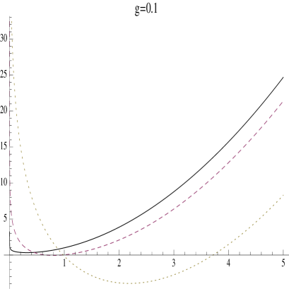
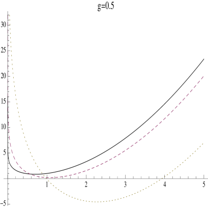
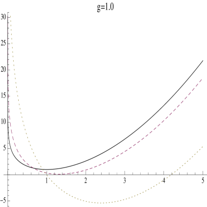
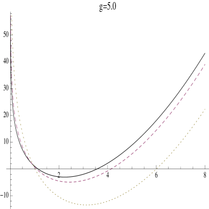
Figure 1: Plots of $U_{\ell}(x)$ versus $x$ for the L1 type FPE with different values of $g$ and $\ell=0$ (solid curve), $1$ (dashed curve) and $5$ (dotted curve)

Below we shall present some numerical results in order to see how the deforming function $\xi_{\ell}(\eta;g)$ modifies the behavior of the drift-diffusion system. Since the diffusion coefficient here is fixed, and the deformation of the system is mainly through the change in the drift coefficient, it suffices to see how the drift potential is deformed as $\ell$ changes. This we plot in Fig. 1 for the L1 type Laguerre systems. The L2 systems behave similarly, and will not be depicted here. Four sets of values of $g$ are shown, namely, $g=0.1,0.5,1.0$ and $5.0$. For each value of $g$, we plot $U_{\ell}(x)$ with $\ell=0$ (the undeformed case), $1$ and $5$.

Since the drift coefficient is related to the negative slope of $U_{\ell}(x)$, one can gain some qualitative understanding of how the peak of the probability density moves just from the sign of the slope of $U_{\ell}(x)$. The reason is as follows. Let us consider the current density $J(x,t)$ near the peak, where the slope of the probability density function is very small, $\partial P(x,t)/\partial x\approx 0$. From eq. (2.2), one has

$$J(x,t)_{\rm peak}\approx-\left(\frac{\partial U_{\ell}(x)}{\partial x}\,P(x,t)\right)_{\rm peak}.$$ (3.26)

As $P(x,t)>0$ near the peak, eq. (3.26) implies that the peak tends to move to the right (left) when it is at a position $x$ such that $\partial U_{\ell}(x)/\partial x$ is negative (positive), until the stationary distribution is reached.

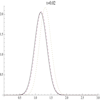
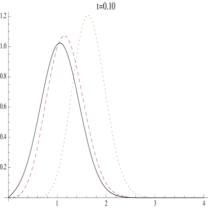
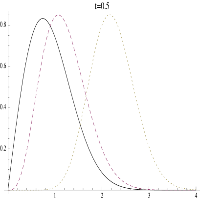
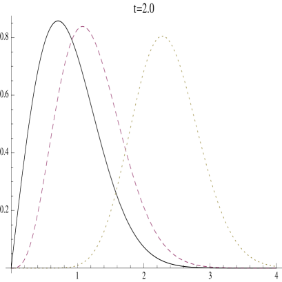
Figure 2: Plots of $\mathcal{P}(x,t)$ versus $x$ for the L1 FPE with different values of $t$ and $g=0.5,x_{0}=1.2$, $\ell=0$ (solid curve), $1$ (dashed curve) and $5$ (dotted curve). Eighty terms in the series in eq. (3.23) were used. The curves shown in the last sub-figure are the stationary distributions for the respective value of $\ell$.

From Fig. 1 one sees that for the values of $g$ considered, the presence of parameter $\ell$ generally makes the slope of $U_{\ell}(x)$ more negative near the left wall $x=0$. So in the deformed systems, the peaks tend to move faster to the right. Also, there can be sign change of the slope of the drift potential in certain region near the left wall. In such region, the peak of the probability density function will move in different directions for different $\ell$. To illustrate this, we consider the system with $g=0.5$. As mentioned before, the $\ell=0$ case with $g=0.5$ correspond to the well-known Rayleigh process. From Fig. 1 we see that at $x_{0}=1.2$, the sign of the slope of $U_{5}(x)$ is different from those of $U_{0}(x)$ and $U_{1}(x)$. Thus one expects that for the initial profile $P(x,0)=\delta(x-x_{0})$ with the peak initially located at $x_{0}=1.2$, the peak will move to the right for $\ell=5$ system, while for the other two values of $\ell$, the peak will move to the left. This is indeed the case as shown in Fig. 2. We note here that the graphs shown in Fig. 2 for $t=2.0$ are already the stationary distributions of the respective cases.

IV FPEs with Exceptional Jacobi polynomials

We now present new exactly solvable FPEs related to the exceptional Jacobi polynomials. We shall call these the generalized Jacobi processes. Here we will be brief, as the method of construction of these systems is the same as that discussed in the previous section.

With appropriate redefinition, one can always set the domain of the basic variable to be $x\in[0,\pi/2]$. The trigonometric Darboux-Pöschl-Teller potential has two parameters $\bm{\lambda}=(g,h)$ ($g>0$, $h>0$) and is defined by the prepotential ($\ell=1,2,\ldots$)

$$w_{0}(x;g,h)=g\log\sin x+h\log\cos x,\quad 0<x<\frac{\pi}{2}.$$ (4.27)

The corresponding deformation of the system is given by the prepotential

$$w_{\ell}(x;g,h)=(g+\ell)\log\sin x+(h+\ell)\log\cos x+\log\frac{\xi_{\ell}(\eta;g+1,h+1)}{\xi_{\ell}(\eta;g,h)},$$ (4.28)

where $\eta(x)=\cos 2x$. The deforming function is defined by

$$\xi_{\ell}(\eta;g,h)=\left\{\begin{array}[]{ll}P_{\ell}^{(g+\ell-\frac{3}{2},-h-\ell-\frac{1}{2})}(\eta),\ \ g>h>0&:\text{J1}\\ P_{\ell}^{(-g-\ell-\frac{1}{2},h+\ell-\frac{3}{2})}(\eta),\ \ h>g>0&:\text{J2}\end{array}\right.,$$ (4.31)

where $P_{n}^{(\alpha,\beta)}(x)$ are the classical Jacobi polynomials.

The drift coefficients of these systems are

$$D^{(1)}(x)=2(g+\ell)\cot x-2(h+\ell)\tan x-2\sin(2x)\left(\frac{\partial_{\eta}\xi_{\ell}(\eta;g+1,h+1)}{\xi_{\ell}(\eta;g+1,h+1)}-\frac{\partial_{\eta}\xi_{\ell}(\eta;g,h)}{\xi_{\ell}(\eta;g,h)}\right).$$ (4.32)

The PDF of these systems are again given by eq. (2.10). The basic data needed in the formula are HOS :

$$\mathcal{E}_{\ell,n}(g,h)=4n(n+g+h+2\ell),$$

$$\phi_{\ell,n}(x;g,h)=\phi_{\ell}(x;g,h)P_{\ell,n}(\eta;g,h),\quad\phi_{\ell}(x;g,h)=\frac{(\sin x)^{g+\ell}(\cos x)^{h+\ell}}{\xi_{\ell}(\eta;g,h)},$$

$$N_{n}(g,h)=\left[\frac{2\,n!\,(2n+g+h)\Gamma(n+g+h)}{\Gamma(n+g+\frac{1}{2})\Gamma(n+h+\frac{1}{2})}\right]^{\frac{1}{2}},$$

$$N^{2}_{\ell,n}(g,h)=\,N^{2}_{n}(g+\ell,h+\ell)\times\left\{\begin{array}[]{ll}\frac{(n+h+\frac{1}{2})(n+g+\ell-\frac{1}{2})}{(n+h+\ell+\frac{1}{2})(n+g+2\ell-\frac{1}{2})}&:\text{J1}\\[4.0pt] \frac{(n+g+\frac{1}{2})(n+h+\ell-\frac{1}{2})}{(n+g+\ell+\frac{1}{2})(n+h+2\ell-\frac{1}{2})}&:\text{J2}\end{array}\right.,$$ (4.35)

$$P_{\ell,n}(\eta;g,h)=\left\{\begin{array}[]{ll}(n+h+\frac{1}{2})^{-1}\bigl{\{}(h+\frac{1}{2})\xi_{\ell}(\eta;g+1,h+1)P_{n}^{(g+\ell-\frac{3}{2},h+\ell+\frac{1}{2})}(\eta)&\\ \phantom{(n+h+\frac{1}{2})^{-1}\bigl{(}}+(1+\eta)\xi_{\ell}(\eta;g,h)\partial_{\eta}P_{n}^{(g+\ell-\frac{3}{2},h+\ell+\frac{1}{2})}(\eta)\bigr{\}}&:\text{J1}\\[2.0pt] (n+g+\frac{1}{2})^{-1}\bigl{\{}(g+\frac{1}{2})\xi_{\ell}(\eta;g+1,h+1)P_{n}^{(g+\ell+\frac{1}{2},h+\ell-\frac{3}{2})}(\eta)&\\ \phantom{(n+g+\frac{1}{2})^{-1}\bigl{(}}-(1-\eta)\xi_{\ell}(\eta;g,h)\partial_{\eta}P_{n}^{(g+\ell+\frac{1}{2},h+\ell-\frac{3}{2})}(\eta)\bigr{\}}&:\text{J2}\end{array}\right..\hskip 5.69054pt$$ (4.40)

As explained in OS1 ; HOS , the exceptional J1 and J2 orthogonal polynomials are ‘mirror images’ of each other, reflecting the parity property $P_{n}^{(\alpha,\beta)}(-\eta)=(-1)^{n}P_{n}^{(\beta,\alpha)}(\eta)$ of the Jacobi polynomial.

Below we discuss some numerical results for the J2 systems. In Fig. 3 we plot the drift potentials $U_{\ell}(x)$ for various sets of parameters.

Figs. 3(a) and 3(b) show how $U_{\ell}(x)$ changes as $\ell$ changes at fixed values of $g$ and $h$. In (a) the difference between $h$ and $g$ is small, and the graphs of $U_{\ell}(x)$ appear nearly symmetric with respect to the mid-point $x=\pi/4$, but with the absolute value of the slope becoming larger at higher $\ell$. So the probability density is pushed faster towards the central region of the well at higher $\ell$. In (b) $h$ is much larger than $g$, and one sees that there can be difference in the signs of the slopes of the drift potential near the left wall. The effect of the sign change is depicted in Fig. 4.

In Figs. 3(c) and 3(d), we show the change in $U_{\ell}(x)$ (at fixed value of $\ell$) when either $g$ or $h$ is changed while the other is kept constant. It is seen that $U_{\ell}(x)$ becomes steeper near the left (right) wall as $g$ ($h$) becomes larger at fixed $h$ ($g$). This implies the probability density function near the left (right) wall is pushed faster towards the right (left) at larger $g$ ($h$) at fixed $h$ ($g$).

In Fig. 4 the time evolution of the probably density function is depicted for the three cases shown in Fig. 3(b). It has been noted that at some points , the slope of $U_{\ell}(x)$ can have different signs at different values of $\ell$ (at fixed $g$ and $h$). For instance, at $x_{0}=0.3$, the slope is positive for $\ell=0$, and are negative for at $\ell=10$ and $15$. If the initial profile peaks at $x_{0}=0.3$, one expects from the signs of the slopes of $U_{\ell}(x)$ that the peak will move towards the left wall for the non-deformed system, and 0towards the right for the other two deformed cases. Fig. 4 shows that this is indeed the case.

V Summary

We have presented four types of infinitely many exactly solvable FPE’s which are the generalised, or deformed versions of the Rayleigh process and the Jacobi process. They are related to the newly discovered exceptional orthogonal polynomials. These new polynomials have the remarkable properties that they start with degree $\ell=1,2\ldots,$ polynomials instead of a constant, and yet they still form complete sets with respect to some positive-definite measure. In some sense they are deformation of the classical Laguerre and Jacobi polynomials. The quantal systems that involve these new polynomials are the deformed radial oscillator and the trigonometric Darboux-Pöschl-Teller potential. Using the transformation between FPE and the Schrödinger equation, we obtained the corresponding FPE’s, which are deformations of the Rayleigh process and the Jacobi process. We have shown numerically how the deformation modify the drift coefficient of the FPE, and hence the evolution of the probability density function. It gives the possibility to manipulate evolution of stochastic processes by suitable choice of a deforming function.

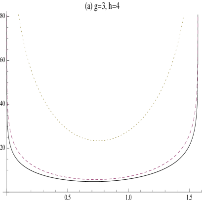
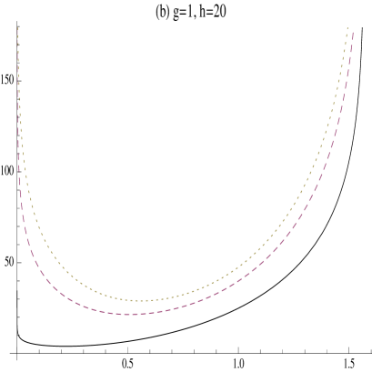
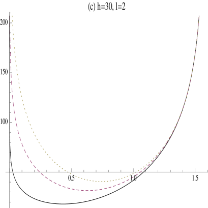
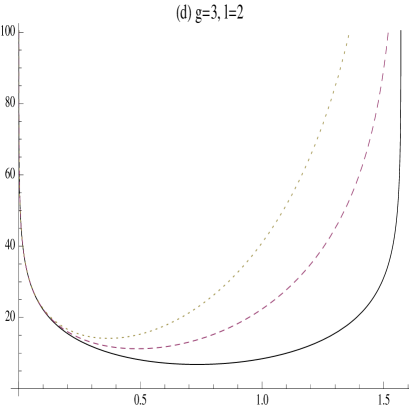
Figure 3: Plots of $U_{\ell}(x)$ versus $x$ for J2 type FPE for : (a) $g=3,h=4$, $\ell=0$ (solid curve), $1$ (dashed curve) and $15$ (dotted curve); (b) $g=1,h=20$, $\ell=0$ (solid curve), $10$ (dashed curve) and $15$ (dotted curve); (c) $h=30,\ell=2$, $g=5$ (solid curve), $15$ (dashed curve) and $25$ (dotted curve); and (d) $g=3,\ell=2$, $h=4$ (solid curve), $15$ (dashed curve) and $30$ (dotted curve)

.

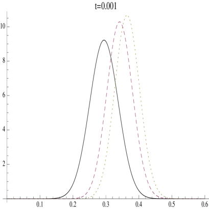
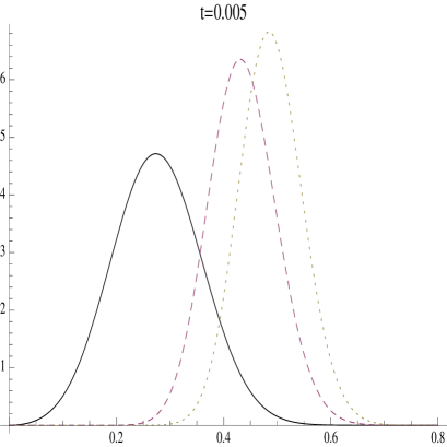
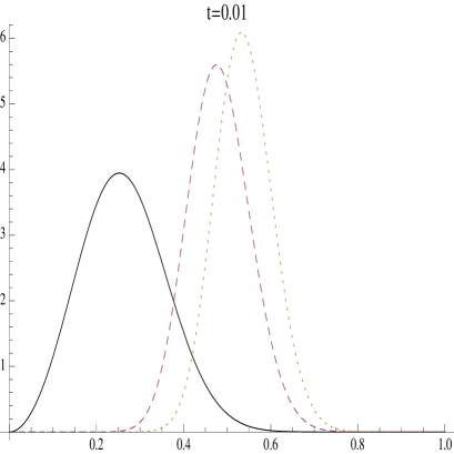
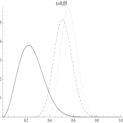
Figure 4: Plots of $\mathcal{P}(x,t)$ versus $x$ for the J2 FPE with different values of $t$ and $g=1,h=20,x_{0}=0.3$, $\ell=0$ (solid curve), $10$ (dashed curve) and $15$ (dotted curve). Fifty terms in the series in eq. (2.10) were used. The curves shown in the last sub-figure are the stationary distributions for the respective value of $\ell$.