UT-12-22

Virasoro constraint for Nekrasov instanton partition function
Shoichi Kanno, Yutaka Matsuo and Hong Zhang
Department of Physics, The University of Tokyo
Hongo 7-3-1, Bunkyo-ku, Tokyo 113-0033, Japan

We show that Nekrasov instanton partition function for $SU(N)$ gauge theories satisfies recursion relations in the form of $U(1)+$Virasoro constraints when $\beta=1$. The constraints give a direct support for AGT conjecture for general quiver gauge theories.

1 Introduction and Summary

Some years ago, Nekrasov and his collaborators [1] found an exact form of the instanton partition functions of $\mathcal{N}=2$ supersymmetric gauge theories in omega background with two deformation parameters $\epsilon_{1},\epsilon_{2}$. It became a milestone in the understanding of supersymmetric gauge theories and their connection with 2D integrable system and initialized the later developments (see for example, [2, 3]).

In this paper, along the line of such developments, we claim that there exist simple recursion formulae for Nekrasov’s instanton partition function for $SU(N)$ gauge theories with $\beta=-\epsilon_{2}/\epsilon_{1}=1$ written in the following form:

$$\sum_{\vec{Y}^{\prime},\vec{W}^{\prime}}(\hat{J}_{n})_{\vec{Y},\vec{W}}^{\vec{Y}^{\prime},\vec{W}^{\prime}}Z_{\vec{Y}^{\prime},\vec{W}^{\prime}}=0\,,\qquad\sum_{\vec{Y}^{\prime},\vec{W}^{\prime}}(\hat{L}_{n})_{\vec{Y},\vec{W}}^{\vec{Y}^{\prime},\vec{W}^{\prime}}Z_{\vec{Y}^{\prime},\vec{W}^{\prime}}=0\,,$$ (1)

where $\hat{J}_{n}$ and $\hat{L}_{n}$ ($n\in\mathbf{Z}$) are infinite dimensional matrices which satisfy Virasoro + U(1) current algebra without central extension,

$$[\hat{J}_{n},\hat{J}_{m}]=0,\quad[\hat{L}_{n},\hat{J}_{m}]=-m\hat{J}_{n+m},\quad[\hat{L}_{n},\hat{L}_{m}]=(n-m)\hat{L}_{n+m}\,.$$ (2)

The indices $\vec{Y},\vec{W}$ are collections of $N$ Young diagrams, for example, $\vec{Y}=(Y_{1},\cdots,Y_{N})$. $Z_{\vec{Y},\vec{W}}$ is a part of the instanton partition function consisting of the contribution of vector and bifundamental multiplets. Precise forms of $\hat{J}_{n},\hat{L}_{n},Z_{\vec{Y},\vec{W}}$ will be given in the text. We conjecture that the relations are part of more general $\mathcal{W}_{1+\infty}$ algebra where (2) become the subalgebra.

The constraint equations give a direct support to ($SU(N)$ generalization of) AGT conjecture [2] which suggests the partition functions of $\mathcal{N}=2$ theories equal to the conformal block functions of Liouville (Toda) field theory. As we will review in next section, the instanton partition function for $SU(N)\times\cdots\times SU(N)$ quiver gauge theory is written out of $Z$ in (1), and (2) implies the existence of conformal Ward identity in the conformal block functions. One remarkable feature is that the proof is not restricted by the number of boxes of Young diagrams but holds in all orders analytically.

The constraint of the form (1) appeared in various contexts in string theory. A famous example is the matrix model which describes two dimensional gravity (Virasoro constraint [4, 5] and $\mathcal{W}_{1+\infty}$ constraint [6, 7]). Given the intimate relation between the matrix model and AGT conjecture[8], the existence of such relation is quite natural.

We organize the paper as follows. In section 2, we define the Nekrasov function $Z_{\vec{Y},\vec{W}}$ in (1). It is a building block of instanton partition function for linear quiver gauge theories. In section 3, we propose a formula which represents $Z_{\vec{Y}\vec{W}}$ as a 3-point function of conformal field theory. While it is written in terms of free fermions, the direct calculation of the correlation function is nontrivial since there is room for inserting screening operators. Instead of directly computing the correlator, we show the conformal Ward identity written in the form (2). Finally in section 4, we give a direct proof of such recursion formula in terms of Nekrasov function. Since the proof is technical and lengthy, we write some explicit computation in the appendix.

2 Nekrasov partition function

In this paper, we focus on the linear quiver gauge theories with gauge group $SU(N_{1})\times\cdots\times SU(N_{n})$ (Figure 1).

Figure 1: Linear quiver

For this case, Nekrasov partition function is written in the form of matrix multiplication [2, 9],

$$Z^{\mathrm{Nek}}=\sum_{\vec{Y}^{(1)},\cdots,\vec{Y}^{(n)}}q_{i}^{|\vec{Y}^{(i)}|}\bar{V}_{\vec{Y}^{(1)}}\cdot Z_{\vec{Y}^{(1)}\vec{Y}^{(2)}}\cdots Z_{\vec{Y}^{(n-1)}\vec{Y}^{(n)}}\cdot V_{\vec{Y}^{(n)}}\,.$$ (3)

Here $q_{i}=e^{2\pi i\tau_{i}}$ describes the coupling constant $\tau_{i}$ for $i^{\mathrm{th}}$ gauge group $SU(N_{i})$. Sets of Young tables $\vec{Y}^{(i)}=(Y^{(i)}_{1},\cdots,Y^{(i)}_{N_{i}})$ are used to label the contribution from fixed points of the localization technique and $|\vec{Y}^{(i)}|=\sum_{p=1}^{N_{i}}|Y^{(i)}_{p}|$ is the sum of the number of boxes for each Young diagram. Each “matrix” $Z$ or “vector” $V,\bar{V}$ contains the information of vacuum expectation value for vector multiplet $\vec{a}^{(i)}$ associated with each gauge group $SU(N_{i})$, the mass for $SU(N_{i})$-$SU(N_{i+1})$ bifundamental multiplet $\mu^{(i)}$, and the mass for fundamental (anti-fundamental) multiplet $\vec{\lambda}$, ($\vec{\lambda}^{\prime}$). They are explicitly written in terms of a function $Z$,

$$Z_{\vec{Y}^{(i)}\vec{Y}^{(i+1)}} = Z(\vec{a}^{(i)},\vec{Y}^{(i)};\vec{a}^{(i+1)},\vec{Y}^{(i+1)};\mu^{(i)}),$$ (4)

$$\bar{V}_{\vec{Y}^{(1)}} = Z(\vec{\lambda},\vec{\emptyset};\vec{a}^{(1)},\vec{Y}^{(1)};\mu^{(0)}),$$ (5)

$$V_{\vec{Y}^{(n)}} = Z(\vec{a}^{(n)},\vec{Y}^{(n)};\vec{\lambda}^{\prime},\vec{\emptyset};\mu^{(n)}),$$ (6)

where $\vec{\emptyset}$ is a set of null Young diagrams $(\emptyset,\cdots,\emptyset)$ and

$$Z(\vec{a},\vec{Y};\vec{b},\vec{W};\mu) = \mathbf{z}_{\mathrm{vect}}(\vec{a},\vec{Y})\bar{\mathbf{z}}_{\mathrm{vect}}(\vec{b},\vec{W})z_{\mathrm{bifund}}(\vec{a},\vec{Y};\vec{b},\vec{W};\mu)\,,$$ (7)

$$\mathbf{z}_{\mathrm{vect}}(\vec{a},\vec{Y}) = \prod_{p,q=1}^{N}G_{Y_{p},Y_{q}}(a_{p}-a_{q})^{-1}\,,$$ (8)

$$\bar{\mathbf{z}}_{\mathrm{vect}}(\vec{a},\vec{Y}) = \prod_{p,q=1}^{N}(-1)^{|Y_{q}|}G_{Y_{q},Y_{p}}(1-\beta-a_{p}+a_{q})^{-1}\,,$$ (9)

$$z_{\mathrm{bifund}}(\vec{a},\vec{Y};\vec{b},\vec{W};\mu) = \prod_{p,q=1}^{N}(-1)^{|W_{q}|}G_{Y_{p},W_{q}}(a_{p}-b_{q}-\mu)G_{W_{q},Y_{p}}(1-\beta-a_{p}+b_{q}+\mu)\,,$$ (10)

$$G_{A,B}(x) := \prod_{(i,j)\in A}(x+\beta(({}^{T}A)_{j}-i+1)+((B)_{i}-j))\,.$$ (11)

$\mathbf{z}_{\mathrm{vect}}$ and $\bar{\mathbf{z}}_{\mathrm{vect}}$ are related to the usual factor for the vector multiplet as $z_{\mathrm{vect}}(\vec{a},\vec{Y})=\mathbf{z}_{\mathrm{vect}}(\vec{a},\vec{Y})\cdot\bar{\mathbf{z}}_{\mathrm{vect}}(\vec{a},\vec{Y})$. ${}^{\mathtt{T}}\!A$ is the transpose of a Young table $A$, $(i,j)$ is the coordinate of a box in the Young diagram $A$ and $(A)_{i}$ (resp. ${}^{\mathtt{T}}\!(A)_{j}$) represents the height of $i^{\mathrm{th}}$ colomn (resp. the length of $j^{\mathrm{th}}$ row). See Figure 2 for the illustration.

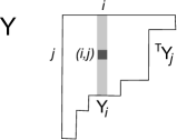
Figure 2: Young diagram

For technical reasons, we restrict our analysis to $\beta=1$ case and derive the $U(1)$+Virasoro constraint for $Z(\vec{a},\vec{Y};\vec{b},\vec{W};\mu)$ with $N_{i}=N_{i+1}$. We will argue that similar constraints exist also for $V_{\vec{Y}},\bar{V}_{\vec{Y}}$. They can be interpreted as a proof of $U(1)$+conformal symmetry in Nekrasov function.

3 2D CFT

3.1 A conjectured relation

The $SU(N)$ generalization of AGT conjecture implies that the partition function (3) can be written as the conformal block of $n+3$ point function of $SU(N)$ Toda field theory [10, 11] where the Hilbert space $\mathcal{H}$ is described by chiral $W_{n}$ algebra with $U(1)$ factor.

We write the conformal block in Figure 3.

Figure 3: Conformal block and correspondence with Nekrasov factor

It can be reduced to the multiplication of three point functions by inserting a complete basis of the Hilbert space at the intermediate channel. In Figure 3, insertion points of such operators are depicted by arrows. In $W_{n}$ +$U(1)$ system, the basis of the Hilbert space is labeled by $N$ Young tables $\vec{Y}$. Then it may be possible to choose such basis such that the factor $Z_{\vec{Y},\vec{W}}$ in the previous section may be rewritten as $Z_{\vec{Y},\vec{W}}\sim\langle\vec{Y}|V(1)|\vec{W}\rangle$ with some vertex operator $V$. The existence of such basis was formally claimed in [12, 13] for general $\beta$ in terms of Jack polynomial, but the explicit form was not given except for some simple examples.

An exceptional case occurs when $\beta=1$ and the system is described by $N$ pairs of free fermions. In this case, there is a reasonable guess on the explicit form of $|\vec{Y},\vec{a}\rangle$ [14, 15] as a product of Schur polynomials, namely $|\vec{Y}\rangle\sim\prod_{p=1}^{N}\chi_{Y^{(p)}}$. (See also [16] for a similar analysis.) In the following, we will provide more precise definition of such states in the Hilbert space of free fermion including the background charges. The formula we would like to establish is

$$Z(-\vec{a},\vec{Y};-\vec{b},\vec{W};\mu)=\langle\!\langle\vec{Y},\vec{a}+\nu\vec{e}|V_{\kappa}(1)|\vec{W},\vec{b}+(\nu-\mu)\vec{e}\rangle\!\rangle\,,$$ (12)

where $V_{\kappa}$ is a vertex operator and $\vec{e}=(1,1,\dots,1)$. The parameter $\nu$ is arbitrary. The vertex operator must has a special form of a momentum $(\kappa,0,\cdots,0)$ to satisfy the Virasoro constraint, where $\kappa$ is determined by the $U(1)$ charge conservation,

$$\sum_{i}(a_{i}+\nu)=-\kappa+\sum_{j}(b_{j}+\nu-\mu).$$ (13)

The number of parameters in gauge theory and CFT is matched up to the irrelevant parameter $\nu$. Precise definitions of the basis $|\vec{W},\vec{\lambda}\rangle$, the vertex operator $V_{\kappa}$ and the inner product $\langle\!\langle\cdot|\cdot\rangle\!\rangle$ are explained in the following subsections.

3.2 Free fermion and vertex operator

We start from the definition of fermions,

$$\bar{\psi}^{(p)}(z)=\sum_{n\in{\bf Z}}\bar{\psi}^{(p)}_{n}z^{-n-\lambda_{p}-1}\,,\;\;\;\psi^{(p)}(z)=\sum_{n\in{\bf Z}}\psi^{(p)}_{n}z^{-n+\lambda_{p}}\,,\quad p=1,\cdots,N,\quad z\in\mathbf{C}$$ (14)

with anti-commutation relation, $\{\bar{\psi}^{(p)}_{n},\psi^{(q)}_{m}\}=\delta_{p,q}\delta_{n+m,0}$. We note that there are extra parameters $\vec{\lambda}\in\mathbf{R}^{N}$ which represent the shift of the usual mode expansion of fermion. We define the vacuum as, $|{\vec{\lambda}}\rangle=\otimes_{p=1}^{N}|\lambda^{(p)}\rangle$,

$$\bar{\psi}^{(p)}_{n}|{\vec{\lambda}}\rangle=\psi^{(p)}_{m}|{\vec{\lambda}}\rangle=0\;\;\;(n\geq 0,m>0),\quad\vec{\lambda}=(\lambda^{(1)},\cdots,\lambda^{(N)})\,.$$ (15)

The parameters $\vec{\lambda}$ represent the fermion sea levels. Similarly, the bra vacuum $\langle{\vec{\lambda}}|=\otimes_{p=1}^{N}\langle{\lambda^{(p)}}|$ is defined by

$$\langle{\vec{\lambda}}|\bar{\psi}^{(p)}_{n}=\langle{\vec{\lambda}}|\psi^{(p)}_{m}=0\;\;\;(n<0,m\leq 0),\quad\vec{\lambda}=(\lambda^{(1)},\cdots,\lambda^{(N)})\,.$$ (16)

In formula (12), the bra state has different sea level (say $\vec{\mu}$) in general. In such cases, we need redefine fermion mode expansion as $\psi^{(p)}(z)=\sum_{n\in{\bf Z}}\psi^{(p)}_{n}z^{-n+\lambda_{p}}=\sum_{n\in{\bf Z}}\tilde{\psi}_{n}^{(p)}z^{-n+\mu_{p}}$ and define the bra vacuum in terms of $\tilde{\psi}$. The Hermitian conjugate is defined as $(|{\vec{\lambda}}\rangle)^{\dagger}=\langle{\vec{\lambda}}|$ and $\psi_{n}^{\dagger}=\bar{\psi}_{-n}$. This is consistent with the shift of label by the change of vacuum.

With this preparation, the basis used in (12) is (after translated in the fermion basis),

$$|\vec{Y},\vec{\lambda}\rangle = \otimes_{p=1}^{N}\left(\bar{\psi}^{(p)}_{-\bar{r}_{1}^{(p)}}\bar{\psi}^{(p)}_{-\bar{r}_{2}^{(p)}}\cdots\bar{\psi}^{(p)}_{-\bar{r}_{s_{1}}^{(p)}}|\lambda^{(p)},-s_{1}\rangle\right),\quad|\lambda^{(p)},-s_{1}\rangle=\psi_{-s_{1}+1}^{(p)}\cdots\psi_{-1}^{(p)}\psi_{0}^{(p)}|\lambda^{(p)}\rangle$$ (17)

$$= (-1)^{|\vec{Y}|}\otimes_{p=1}^{N}\left(\psi^{(p)}_{-\bar{s}_{1}^{(p)}}\psi^{(p)}_{-\bar{s}_{2}^{(p)}}\cdots\psi^{(p)}_{-\bar{s}_{r_{1}}^{(p)}}|\lambda^{(p)},r_{p}\rangle\right),\quad|\lambda^{(p)},r_{1}\rangle=\bar{\psi}_{-r_{1}}^{(p)}\cdots\bar{\psi}_{-1}^{(p)}|\lambda^{(p)}\rangle$$ (18)

$$\langle{\vec{Y},\vec{\lambda}}| = (|{\vec{Y},\vec{\lambda}}\rangle)^{\dagger}$$ (19)

Here we represent a Young diagram $Y_{p}$ by the number of each row $r_{\sigma}^{(p)}=({}^{\mathtt{T}}Y_{p})_{\sigma}$ or the number of each columns $s_{\sigma}^{(p)}=(Y_{p})_{\sigma}$. The parameters with bar are $\bar{r}_{\sigma}^{(p)}=r_{\sigma}^{(p)}-\sigma+1$ and $\bar{s}_{\sigma}^{(p)}=s_{\sigma}^{(p)}-\sigma$. These states give a natural basis of the Hilbert space with fixed fermion number. By construction, they are orthonormal $\langle\vec{Y},\vec{a}|\vec{W},\vec{b}\rangle=\delta_{\vec{Y},\vec{W}}\delta_{\vec{a},\vec{b}}$ .

We define the vertex operator $V_{\kappa}$ in (12) by standard bozonization technique. We write,

$$\psi^{(p)}(z)=:e^{-\phi_{p}(z)}:,\quad\bar{\psi}^{(p)}(z)=:e^{\phi_{p}(z)}:\,,$$ (20)

with

$$\phi_{p}(z)=x_{p}+a_{0}\log z-\sum_{n\neq 0}\frac{a^{(p)}_{n}}{n}z^{-n}\,,\quad[a^{(p)}_{n},a^{(q)}_{m}]=n\delta_{p,q}\delta_{n+m,0},\ [x_{p},a^{(q)}_{0}]=\delta_{p,q}\,.$$ (21)

The vacuum and the fermionic basis (17) is written in a form,

$$|\vec{\lambda}\rangle=\lim_{z\rightarrow 0}:e^{-\sum_{p}\lambda_{p}\phi_{p}(z)}:|\vec{0}\rangle,\quad|\vec{Y},\vec{\lambda}\rangle=\prod_{p}\chi_{Y^{(p)}}(a^{(p)}_{-n})|\vec{\lambda}\rangle\,.$$ (22)

Here $\chi_{Y^{(p)}}(a^{(p)}_{-n})$ is Schur polynomial expressed in terms of power sum $\mathbf{p}_{n}=\sum_{i}(x_{i})^{n}$ and each $\mathbf{p}_{n}$ is replaced by $a^{(p)}_{-n}$. While the second expression is not used in the following, it is this expression that appeared in the literature [13, 14, 15]. The vertex operator in (12) is written as,

$$V_{\vec{\kappa}}(z)=:e^{\sum_{p}\kappa_{p}\phi_{p}(z)}:\,.$$ (23)

Here we have to be careful in the definition of the inner product (12). If we interpret it as the correlation function for free fields, the momentum for each fermion pair should be separately conserved, namely,

$$\langle\vec{Y},\vec{a}+\nu\vec{e}|V_{\vec{\kappa}}(1)|\vec{W},\vec{b}+(\nu-\mu)\vec{e}\rangle\propto\delta_{\vec{a},\vec{\kappa}+\vec{b}-\mu\vec{e}}\,.$$ (24)

On the other hand, in the Nekrasov formula, there is no such constraints. So we have to interpret the inner product not as that of free fields but the conformal block of $W_{n}$ algebra +$U(1)$ current algebra as in the literature. The difference between the two is that one may insert the screening operators to recover the conservation of momentum. While it is not explicitly written in (12), the insertion of screening operators is implicitly assumed. In general it gives a generalized Selberg integral of Schur functions [21, 19, 20] when a set of Young tables is empty, namely $\vec{W}=\vec{\emptyset}$. For this case, the integration path of the screening currents may be taken as paths connecting $0$ to $1$.

In our case where both $\vec{Y},\vec{W}$ are not empty, the definition of such integration is even more tricky. We will not attempt to do this in this paper but use (12) as a formal expression to derive the recursion formulae that Nekrasov function should obey. The proof of the identity does not use the definition (12) but the properties of Nekrasov function alone.

Another point we have to pay attention to is the momentum of the vertex operator. As we mentioned in the previous subsection, we need to take it as a special form $\vec{\kappa}=(\kappa,0,\cdots,0)$. This is required by the closure of conformal Ward identity for $W$ algebra [10, 11]. We will come back to this issue later.

3.3 $\mathcal{W}_{1+\infty}$ algebra

For $\beta=1$ case, $W_{N}$ +$U(1)$ current algebra is enhanced to $\mathcal{W}_{1+\infty}$ algebra , which is a quantization of the algebra of higher differential operators. For a differential operator $z^{n}D^{m}$ ($D=z\frac{\partial}{\partial z}$), we define a generator $\mathcal{W}(z^{n}e^{xD}):=\sum_{m=0}^{\infty}\frac{x^{m}}{m!}\mathcal{W}(z^{n}D^{m})$ as,

$$\mathcal{W}(z^{n}e^{xD}) = \frac{1}{2\pi i}\oint_{z=0}dz\sum_{p=1}^{N}z^{n}:\bar{\psi}^{(p)}(z)e^{xD}\psi^{(p)}(z):-\sum_{p=1}^{N}\frac{e^{\lambda_{p}x}-1}{e^{x}-1}\delta_{n,0}$$ (25)

$$= \sum_{p=1}^{N}\sum_{\ell\in\mathbf{Z}}e^{x(\ell+\lambda_{p})}:\bar{\psi}^{(p)}_{\ell+n}\psi^{(p)}_{-\ell}:-\sum_{p=1}^{N}\frac{e^{\lambda_{p}x}-1}{e^{x}-1}\delta_{n,0}.$$ (26)

From our definition of the Hermitian conjugation, we see $W(z^{n}D^{m})^{\dagger}=W(z^{-n}(D-n)^{m})$. Their commutation relation is written as,

$$[\mathcal{W}(z^{n}e^{xD}),\mathcal{W}(z^{m}e^{yD})]=(e^{mx}-e^{ny})\mathcal{W}(z^{n+m}e^{(x+y)D})-C\frac{e^{mx}-e^{ny}}{e^{x+y}-1}\delta_{n+m,0}\,,$$ (27)

with $C=N$. The realization (25) gives a unitary representation of $\mathcal{W}_{1+\infty}$ [18]. The $U(1)$ current and Virasoro operators are embedded in $\mathcal{W}_{1+\infty}$ as,

$$J_{n} = \mathcal{W}(z^{n})=\sum_{p=1}^{N}\sum_{m\in\mathbf{Z}}:\bar{\psi}^{(p)}_{n+m}\psi^{(p)}_{-m}:-\delta_{n0}\sum_{p=1}^{N}\lambda_{p},$$ (28)

$$L_{n} = -\mathcal{W}(z^{n}D)-\frac{n+1}{2}\mathcal{W}(z^{n})=-\sum_{p=1}^{N}\sum_{m\in\mathbf{Z}}\frac{n+2m+2\lambda_{p}+1}{2}:\bar{\psi}^{(p)}_{n+m}\psi^{(p)}_{-m}:+\frac{\delta_{n0}}{2}\sum_{p=1}^{N}\lambda_{p}^{2},$$ (29)

which satisfy

$$[J_{n},J_{m}]=N\delta_{n+m,0},\quad[L_{n},J_{m}]=-mJ_{n+m},\quad[L_{n},L_{m}]=(n-m)L_{n+m}+\frac{N}{12}(n^{3}-n)\delta_{n+m,0}\,.$$ (30)

While the bosonized version of $\mathcal{W}_{1+\infty}$ generators are given in a closed form [15], they are in general highly nonlinear. The exceptions are $U(1)$ and Virasoro generators which have the standard form,

$$J_{n}=\frac{1}{2\pi i}\oint_{z=0}dz\sum_{p=1}^{N}z^{n}\partial\phi_{p}(z),\qquad L_{n}=\frac{1}{2\pi i}\oint_{z=0}dz\sum_{p=1}^{N}z^{n+1}\frac{1}{2}:(\partial\phi_{p}(z))^{2}:.$$ (31)

In the following, we treat the inner product (12) as the conformal block of $\mathcal{W}_{1+\infty}$ algebra. The use of $\mathcal{W}_{1+\infty}$ instead of $W_{N}+U(1)$ has definite merit in the simplicity of the expression (25) and the algebra (27) in a closed form.

The screening operators of $\mathcal{W}_{1+\infty}$ mentioned in the previous subsection are written as,

$$S_{pq}=\int_{\mathcal{C}}d\zeta\bar{\psi}^{(p)}(\zeta)\psi^{(q)}(\zeta)\,,$$ (32)

with $p\neq q$. It can be easily established that it commute with all the generators of $\mathcal{W}_{1+\infty}$ algebra as long as the integration contour $\mathcal{C}$ is appropriately chosen [22]. We assume these operators are implicitly inserted in (12). We used a notation $\langle\!\langle\cdot|\cdot\rangle\!\rangle$ to implement this idea,

$$\langle\!\langle\vec{Y},\vec{\lambda}|V_{\kappa}(1)|\vec{W},\vec{\mu}\rangle\!\rangle:=\langle\vec{Y},\vec{\lambda}|V_{\kappa}(1)S_{p_{1}q_{1}}S_{p_{2}q_{2}}\cdots|\vec{W},\vec{\mu}\rangle\,.$$ (33)

Here the right hand side is the inner product of the free fields. The insertions of screening operators change the U(1) charge for each boson in the form $(c_{1},\cdots,c_{N})$ with $\sum_{i=1}^{N}c_{i}=0$. The conservation of momentum for each $\phi_{p}$ can be broken but only their sum is conserved, namely we have (13).

An intriguing feature of the fermion basis (17) is that the action of $\mathcal{W}_{1+\infty}$ generators is written neatly. In particular, they are simultaneous eigenstates of all the commuting generators of $\mathcal{W}_{1+\infty}$,

$$\mathcal{W}(e^{xD})|\vec{Y},\vec{\lambda}\rangle = \Delta(\vec{Y},\vec{\lambda},x)|\vec{Y},\vec{\lambda}\rangle,$$ (34)

$$\Delta(\vec{Y},\vec{\lambda},x) = \sum_{p=1}^{N}\left(\sum_{\sigma_{p}=1}^{s_{p}}\left(e^{-xr^{(p)}_{\sigma_{p}}}-1\right)e^{x(\sigma_{p}-1+\lambda_{p})}\right)-\sum_{p=1}^{N}\frac{e^{\lambda_{p}x}-1}{e^{x}-1}$$ (35)

$$= \sum_{p=1}^{N}\left(\sum_{\sigma_{p}=1}^{r_{p}}\left(1-e^{xs^{(p)}_{\sigma_{p}}}\right)e^{x(-\sigma_{p}+\lambda_{p})}\right)-\sum_{p=1}^{N}\frac{e^{\lambda_{p}x}-1}{e^{x}-1}\,.$$ (36)

In particular,

$$J_{0}|\vec{Y},\vec{\lambda}\rangle=-\sum_{p=1}^{N}\lambda_{p}|\vec{Y},\vec{\lambda}\rangle,\quad L_{0}|\vec{Y},\vec{\lambda}\rangle=\sum_{p=1}^{N}\left(|Y_{p}|+\frac{\lambda_{p}^{2}}{2}\right)|\vec{Y},\vec{\lambda}\rangle\,.$$ (37)

3.4 Construction of the constraints

Now we arrive at the position to explain how to construct the recursion relation of the form (1). The conjectured relation (12), while it is not completely well-defined, gives a good hint. We use the following trivial identity ,

$$0 = \langle\!\langle\vec{Y},\vec{a}+\nu\vec{e}|\mathcal{W}(z^{n}D^{p})V_{\kappa}(1)|\vec{W},\vec{b}+(\nu-\mu)\vec{e}\rangle\!\rangle$$ (38)

$$-\langle\!\langle\vec{Y},\vec{a}+\nu\vec{e}|V_{\kappa}(1)\mathcal{W}(z^{n}D^{p})|\vec{W},\vec{b}+(\nu-\mu)\vec{e}\rangle\!\rangle$$

$$-\langle\!\langle\vec{Y},\vec{a}+\nu\vec{e}|[\mathcal{W}(z^{n}D^{p}),V_{\kappa}(1)]|\vec{W},\vec{b}+(\nu-\mu)\vec{e}\rangle\!\rangle$$

$$= \sum_{\vec{Y}^{\prime},\vec{W}^{\prime}}\hat{\mathcal{W}}(z^{n}D^{p})_{\vec{Y},\vec{W}}^{\vec{Y}^{\prime},\vec{W}^{\prime}}\langle\!\langle\vec{Y}^{\prime},\vec{a}+\nu\vec{e}|V_{\kappa}(1)|\vec{W}^{\prime},\vec{b}+(\nu-\mu)\vec{e}\rangle\!\rangle\,.$$

Here the first two lines can be evaluated by action of $\mathcal{W}(z^{n}D^{p})$ on the bra and ket basis. The third line is given by the commutator with the vertex. As we see these are written as a linear combination of inner product and can be written in the fourth line. The insertion of screening charges does not play any role since they commute with $\mathcal{W}_{1+\infty}$ generators. The coefficients of the recursion relations $\hat{\mathcal{W}}(z^{n}D^{p})_{\vec{Y},\vec{W}}^{\vec{Y}^{\prime},\vec{W}^{\prime}}$ satisfy the $\mathcal{W}_{1+\infty}$ algebra since they are the difference between the action of $\mathcal{W}(z^{n}D^{p})$ on the bra and vertex$+$ket states. The central charges cancel between the two terms.

If the eq.(12) holds, the Nekrasov function should also satisfy the relation, namely,

$$\sum_{\vec{Y}^{\prime},\vec{W}^{\prime}}\hat{\mathcal{W}}(z^{n}D^{p})_{\vec{Y},\vec{W}}^{\vec{Y}^{\prime},\vec{W}^{\prime}}Z(-\vec{a},\vec{Y}^{\prime};-\vec{b},\vec{W}^{\prime};\mu)=0.$$ (39)

This is what we would like to establish in the following.

Actually we meet a technical problem in the computation of $\mathcal{W}(z^{n}D^{p})$ with $p\geq 2$. Since their bosonic realization is highly nonlinear, the commutator with the vertex operator becomes messy. So in this paper, we limit ourselves to focus on safer $U(1)$+Virasoro part ($p=0,1$). We also note that we do not need to derive all the identity of the form (38). Since they form a noncommutative algebra, proving identity of the form (38) for $\mathcal{W}(z^{\pm 1})$ and $\mathcal{W}(z^{\pm n}D)$ $n=1,2$ (i.e. $J_{\pm 1},L_{\pm 1},L_{\pm 2}$) will generate all other constraints. For example, $[\hat{L}_{1},\hat{J}_{1}]=-\hat{J}_{2}$, $[\hat{L}_{2},\hat{L}_{1}]=\hat{L}_{3}$ and so on.

In the following we evaluate the action of $\mathcal{W}_{1+\infty}$ on the basis and the vertex.

Action on bra and ket basis

In order to evaluate the action of $W(z^{n}e^{xD})$ ($n\neq 0$) on $|\vec{Y},\vec{\lambda}\rangle$, a graphic representation (Maya diagram) of $|\vec{Y},\vec{\lambda}\rangle$ [23] is useful. For the simplicity of argument, we take $N=1$ and remove the the index $p$ in (17,18). We take the first expression (17) and rewrite it as,

$$|Y,\lambda\rangle=\bar{\psi}_{-\bar{r}_{1}}\bar{\psi}_{-\bar{r}_{2}}\cdots\bar{\psi}_{-\bar{r}_{s}}\bar{\psi}_{s}\bar{\psi}_{s+1}\cdots\bar{\psi}_{L}|-L,\lambda\rangle\,.$$ (40)

and take $L\rightarrow\infty$ limit. From this representation, we associate a Young diagram $Y$ with a semi-inifinite sequence of integers $S_{Y}=\{\bar{r}_{1},\bar{r}_{2},\cdots,\bar{r}_{s},-s,-s-1,\cdots\}$. We prepare an infinite strip of boxes with integer label and fill the boxes with the integer in $S_{Y}$ (Figure 4 left).

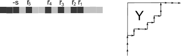
Figure 4: Young diagram and fermion state

It represents the occupation of fermion in each level. To understand the correspondence with the Young diagram $Y$, we associate each black box with vertical up arrow and white box with horizontal right arrow. We connect these arrows for each box from the left on $S_{Y}$. Then the Young diagram shows up in the up/left corner (Figure 4 right). The generator $\mathcal{W}(z^{n}e^{xD})=\sum_{\ell}e^{x(\ell+\lambda)}:\bar{\psi}_{\ell+n}\psi_{-\ell}:$ flips one black box at $\ell$ to white and one white box at $-\ell-n$ to black (if wrong color was filled at each place, it vanishes). It amounts to flipping vertical arrow by horizontal one and vice versa. By analyzing the effect of such flipping, the action of $\mathcal{W}(z^{n}e^{xD})$ on $|Y,\lambda\rangle$ can be summarized as,

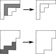
Figure 5: Action of $\mathcal{W}$ on $|Y\rangle$

• For $n>0$ it erases a hook of length $n$ and multiply $(-1)^{v(h)-1}e^{x(\ell+\lambda)}$ where $v(h)$ is the height of the hook. (Figure 5 up) If there are some hooks of length $n$, we sum over all such possibilities.

• For $n<0$ it adds a strip of length $|n|$ and multiply $(-1)^{v(h)-1}e^{x(\ell+\lambda)}$ where $v(h)$ is the height of the strip. (Figure 5 down) As in $n>0$ case, if there are some possibility, we need to add them.

As we explained, in practice we need evaluate only $n=\pm 1,n=\pm 2$ cases. The action of $\mathcal{W}(z^{n}D^{m})$ is much simplified and the explicit form is given in section 4.

Commutator with the vertex

The vertex operator $V_{\kappa}(1)$ is the operator version of state $|\vec{\kappa}\rangle$. As we mentioned, it is restricted to be of the form, $\vec{\kappa}=(\kappa,0,\cdots,0)$ and the vertex is expressed as $e^{\kappa\phi_{1}(1)}$. This is a restricted set of vacuum where we have only two independent states at level one, namely $W(z^{-1})|\vec{\mu}\rangle$ and $W(z^{-1}D)|\vec{\kappa}\rangle$. All other states are related to the second one as, $W(z^{-1}D^{p})|\vec{\kappa}\rangle=\kappa^{p-1}W(z^{-1}D)|\vec{\kappa}\rangle$ for $p\geq 1$. This is the level one degenerate state condition for simple vertex [10, 11] for $\mathcal{W}_{1+\infty}$. In the next section, we show that the vertex to have this form is necessary to have even $U(1)$ and Virasoro constraints.

The derivation of the commutation relation between the vertex and $U(1)$ and Virasoro generator are straightforward since it is a primary field,

$$[J_{n},V_{\kappa}(1)]=\kappa V(1),\quad[L_{n},V_{\kappa}(1)]=\frac{\kappa^{2}(n+1)}{2}V_{\kappa}(1)+\partial V(1)\,.$$ (41)

On the other hand, the operator $W(z^{n}D^{m})$ with $m\geq 2$ is written in terms of boson as $W(z^{n}D^{m})\sim(\partial\phi)^{m+1}$ and the commutation relation with the vertex is not written in a compact form. The exceptional case is $\kappa=\pm 1$ where the vertex operator can be identified with the fermion,

$$[\mathcal{W}(z^{n}D^{m}),\bar{\psi}(\zeta)]=\zeta^{n}D_{\zeta}^{m}\bar{\psi}(\zeta),\qquad[\mathcal{W}(z^{n}D^{m}),\psi(\zeta)]=-(\zeta^{n}D_{\zeta}^{m})^{\dagger}\psi(\zeta)\,.$$ (42)

Except for such cases, the evaluation of recursion formula becomes complicated. While we spent some time to solve this problem, we could not manage to write it in a closed form. Because of this technical issue, we will not analyze $\mathcal{W}(z^{n}D^{m})$ with $m\geq 2$.

4 Proof of $U(1)$/Virasoro constraints

As we mentioned, the derivations of recursion formulae for $J_{\pm 1}$, $L_{\pm 1},L_{\pm 2}$ will be enough to prove (1). We will explicitly show them one by one in this section.

Here, we give a few remarks.

• As a corollary of (1), we can obtain the recursion formulae for $V_{\vec{Y}},\bar{V}_{\vec{Y}}$ in (3) automatically if the reader follow the proof in the following. These can be identified with the Nekrasov partition function $SU(N)$ gauge theory with $2N$ fandamental matters. All we need to do is to restrict $\vec{W}=\vec{\emptyset}$ and restrict the constraints to $J_{1},L_{1},L_{2}$. They are proved by observing, for example, $\mathcal{W}(z^{n}D^{m})|\vec{\emptyset},\vec{b}+(\nu-\mu)\vec{e}\rangle=0$ for $n>0$ in the arguments below. By taking commutator among constraints, it gives rise to a family of constraints of the form,

  $$(\hat{J}_{n})_{\vec{Y}}^{\vec{Y}^{\prime}}V_{\vec{Y}}=(\hat{L}_{n})_{\vec{Y}}^{\vec{Y}^{\prime}}V_{\vec{Y}}=0,$$ (43)

  with $n>0$. This can be regarded as the $U(1)$+Virasoro constraints for fundamental+vector multiplets.

• In the computation below, we will analyze the recursion relation when the rank of $\vec{Y}$ and $\vec{W}$ in (12) can be different, namely $\vec{Y}=(Y_{1},\cdots,Y_{N})$ and $\vec{W}=(W_{1},\cdots,W_{M})$ without requiring $N=M$. In CFT, such possibility is difficult to interpret since it implies we have different number of fermions on the bra and ket states. On the other hand, in the context of linear quiver, it shows up when the ranks of gauge groups are different. While Nekrasov formula exists for such cases $N\neq M$, the interpretation in terms of CFT has been a focus of the literature [24, 25]. Our analysis in the following implies $N=M$ to keep the constraints. This is natural from the viewpoint of CFT. This seems to support the claim in [24] that AGT type conjecture holds only for $SU(N)\times\cdots\times SU(N)$ type quiver.

4.1 $U(1)$

From the explanation in the previous section, the action of $\mathcal{W}(z^{\pm 1}D^{m})$ on the basis $|\vec{Y},\lambda\rangle$ (or $\langle\vec{Y},\lambda|$) is obtained by adding or subtracting one box on one of the Young diagram in $\vec{Y}$ with appropriate coefficient. This can be more explicitly expressed by representing each Young diagram $Y_{p}$ as a set of rectangles (Figure 6).

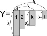
Figure 6: Rectangle decomposition of Young diagram

We denote the Young diagram in the figure as, $Y=[(r_{1},s_{1}),\cdots,(r_{f},s_{f})]$. ($r_{1}<r_{2}<\cdots<r_{f}$, $s_{1}>s_{2}>\cdots>s_{r}$). We write $p^{\mathrm{th}}$ diagram in $\vec{Y},\vec{W}$ as,

$$Y_{p}=[(r^{(p)}_{1},s^{(p)}_{1}),\cdots,(r^{(p)}_{f^{(p)}},s^{(p)}_{f^{(p)}})]\,,\quad W_{p}=[(t^{(p)}_{1},u^{(p)}_{1}),\cdots,(t^{(p)}_{\bar{f}^{(p)}},u^{(p)}_{\bar{f}^{(p)}})]\,.$$ (44)

The addition or the subtraction of a box is expressed on (from) which rectangle the box is added (subtracted). We denote $Y^{(k,+)}$ (resp. $Y^{(k,-)}$) as the diagram by adding (resp. removing) a box in $k^{\mathrm{th}}$ rectangle of $Y$ (Figure 7).

Figure 7: Adding (subtracting) a box to/from Young diagram

With this notation, the first three lines in (38) are evaluated as,

$$\langle\vec{Y},\vec{a}+\nu\vec{e}|J_{1}=\sum_{p=1}^{N}\sum_{k=1}^{f_{p}+1}\langle\vec{Y}^{(k,+),p},\vec{a}+\nu\vec{e}|,$$ (45)

$$[J_{1},V_{\kappa}(1)]=\kappa V(1)\,,$$ (46)

$$J_{1}|\vec{W},\vec{b}+(\nu-\mu)\vec{e}\rangle=\sum_{q=1}^{M}\sum_{l=1}^{\bar{f}_{q}}|\vec{W}^{(l,-),q},\vec{b}+(\nu-\mu)\vec{e}\rangle.$$ (47)

Here $\vec{Y}^{(k,+),p}=(Y_{1},\cdots Y_{p}^{(k,+)},\cdots Y_{N})$ and $\vec{W}^{(k,-),p}=(W_{1},\cdots W_{p}^{(k,-)},\cdots W_{M})$. From these expressions, the coefficient $\hat{J}_{1}$ in the last line of (38) is written as

$$(\hat{J}_{1})_{\vec{Y},\vec{W}}^{\vec{Y}^{\prime},\vec{W}^{\prime}}=\left\{\begin{array}[]{ll}-\kappa&\vec{Y}=\vec{Y}^{\prime},\,\vec{W}=\vec{W}^{\prime}\\ 1&\vec{Y}^{(k,+),p}=\vec{Y}^{\prime},\vec{W}=\vec{W}^{\prime}\\ -1&\vec{W}^{(k,-),p}=\vec{W}^{\prime},\ \vec{Y}=\vec{Y}^{\prime}\\ 0&\mbox{otherwise}\end{array}\right.\,.$$ (52)

Similarly, for $W(z^{-1})=J_{-1}$,

$$(\hat{J}_{-1})_{\vec{Y},\vec{W}}^{\vec{Y}^{\prime},\vec{W}^{\prime}}=\left\{\begin{array}[]{ll}-\kappa&\vec{Y}=\vec{Y}^{\prime},\,\vec{W}=\vec{W}^{\prime}\\ 1&\vec{Y}^{(k,-),p}=\vec{Y}^{\prime},\vec{W}=\vec{W}^{\prime\prime}\\ -1&\vec{W}^{(k,+),p}=\vec{W}^{\prime},\ \vec{Y}=\vec{Y}^{\prime}\\ 0&\mbox{otherwise}\end{array}\right.\,.$$ (57)

We put these explicit forms to (39) and prove the identity. For this purpose, we need evaluate the quantity,

$$Q(\vec{Y}^{\prime},\vec{W}^{\prime};\vec{Y},\vec{W})\equiv\frac{Z(-\vec{a},\vec{Y}^{\prime};-\vec{b},\vec{W}^{\prime};\mu)}{Z(-\vec{a},\vec{Y};-\vec{b},\vec{W};\mu)}\,,$$ (58)

with $\beta=1$. The constraint for $J_{1}$ is written as,

$$\sum_{p=1}^{N}\sum_{k=1}^{f_{p+1}}Q(\vec{Y}^{(k,+),p},\vec{W};\vec{Y},\vec{W})=\kappa+\sum_{q=1}^{M}\sum_{k=1}^{\bar{f}_{p}}Q(\vec{Y},\vec{W}^{(k,-),p};\vec{Y},\vec{W})\,.$$ (59)

Since the proof for $J_{-1}$ is completely parallel, we focus to give the explicit computation for $J_{1}$.

We evaluate the change by the addition and subtraction of a box in Young diagrams in Nekrasov formula. After a lengthy computation (see appendix A for detail), two $Q$’s in (59) are evaluated as,

$$Q(\vec{Y}^{(k,+),p},\vec{W};\vec{Y},\vec{W}) = (-1)^{N+M-1}\prod_{q=1}^{N}\frac{\prod_{l=1}^{f_{q}}A_{(p)k}-B_{(q)l}}{\prod_{(q)l\neq(p)k}^{f_{q}+1}A_{(p)k}-A_{(q)l}}\times\prod_{q=1}^{M}\frac{\prod_{l=1}^{f_{q}+1}A_{(p)k}-C_{(q)l}}{\prod_{l=1}^{f_{q}}A_{(p)k}-D_{(q)l}}\,,$$ (60)

$$Q(\vec{Y},\vec{W}^{(k,-),p};\vec{Y},\vec{W}) = (-1)^{N+M}\prod_{q=1}^{N}\frac{\prod_{l=1}^{f_{q}}D_{(p)k}-B_{(q)l}}{\prod_{l=1}^{f_{q}+1}D_{(p)k}-A_{(q)l}}\times\prod_{q=1}^{M}\frac{\prod_{l=1}^{f_{q}+1}D_{(p)k}-C_{(q)l}}{\prod_{(q)l\neq(p)k}^{f_{q}}D_{(p)k}-D_{(q)l}}\,,$$ (61)

where

$$\begin{array}[]{ll}A_{(p)k}=a_{p}+\nu+s^{(p)}_{k}-r^{(p)}_{k-1},&1\leq p\leq N,\qquad 1\leq k\leq f_{p}+1\,,\\ B_{(p)k}=a_{p}+\nu+s^{(p)}_{k}-r^{(p)}_{k},&1\leq p\leq N,\qquad 1\leq k\leq f_{p}\,,\\ C_{(p)k}=b_{p}+\nu-\mu+u^{(p)}_{k}-t^{(p)}_{k-1},&1\leq p\leq M,\qquad 1\leq k\leq\tilde{f}_{p}+1\,,\\ D_{(p)k}=b_{p}+\nu-\mu+u^{(p)}_{k}-t^{(p)}_{k},&1\leq p\leq M,\qquad 1\leq k\leq\tilde{f}_{p}\,.\end{array}$$ (62)

We further rewrite

$$A_{(1)k},A_{(2)k},\dots,A_{(n)k},D_{(N+1)k},D_{(N+2)k},\dots,D_{(N+M)k}\equiv x_{I},$$ (63)

$$B_{(1)k},B_{(2)k},\dots,B_{(N)k},C_{(N+1)k},C_{(N+2)k},\dots,C_{(N+M)k}\equiv-y_{J}.$$ (64)

The index $I$ goes from $1$ to $\sum_{p=1}^{N}(f_{p}+1)+\sum_{q=1}^{M}\bar{f}_{q}=N+\sum_{p=1}^{N}f_{p}+\sum_{q=1}^{M}\bar{f}_{q}\equiv\mathcal{N}$, whereas $J$ goes from $1$ to $M+\sum_{p=1}^{N}f_{p}+\sum_{q=1}^{M}\bar{f}_{q}\equiv\mathcal{M}$. Two terms in Eq.(59) that contain $Q$ are rewritten in a compact form,

$$\sum_{p=1}^{N}\sum_{k=1}^{f_{p+1}}Q(\vec{Y}^{(k,+),p},\vec{W};\vec{Y},\vec{W})-\sum_{q=1}^{M}\sum_{k=1}^{\bar{f}_{p}}Q(\vec{Y},\vec{W}^{(k,-),p};\vec{Y},\vec{W})$$

$$=(-1)^{N+M-1}\sum_{I=1}^{\mathcal{N}}\frac{\prod_{J=1}^{\mathcal{M}}(x_{I}+y_{J})}{\prod_{J\neq I}^{\mathcal{N}}(x_{I}-x_{J})}\,.$$ (65)

Then one may use an identity (see the appendix B for a proof),

$$\sum_{I=1}^{\mathcal{N}}\frac{\prod_{J=1}^{\mathcal{M}}(x_{I}+y_{J})}{\prod_{J\neq I}^{\mathcal{N}}(x_{I}-x_{J})}=\mbox{Coefficient of $\zeta^{M-N+1}$ of}\quad\frac{\prod_{J=1}^{\mathcal{M}}(\zeta+y_{J})}{\prod_{I=1}^{\mathcal{N}}(\zeta-x_{I})}\,.$$ (66)

In particular, for $\mathcal{N}=\mathcal{M}$ (i.e. $N=M$) the right hand side of (65) gives,

$$-\sum_{I=1}^{\mathcal{N}}(x_{I}+y_{I})=-\sum_{p=1}^{N}(a_{p}-b_{p}+\mu)=\kappa\,.$$ (67)

In the second equality, we use the charge conservation which is derived from the Ward identity for $J_{0}$. This proves the constraint of $J_{1}$ for $N=M$. At the same time, it implies the constraint holds only when $N=M$.

4.2 Virasoro

Next, let us consider Virasoro constraint. The analogs of eqs. (45)-(47) for $L_{1}$ are

$$\langle\vec{Y},\vec{a}+\nu\vec{e}|L_{1}=-\sum_{p=1}^{N}\sum_{k=1}^{f_{p}+1}(a_{p}+\nu+s_{k}^{(p)}-r_{k-1}^{(p)})\langle\vec{Y}^{(k,+),p},\vec{a}+\nu\vec{e}|,$$ (68)

$$[L_{1},V_{\kappa}(1)]=(\partial_{\zeta}+\kappa^{2})V(\zeta)|_{\zeta=1}\,,$$ (69)

$$L_{1}|\vec{W},\vec{b}+(\nu-\mu)\vec{e}\rangle=-\sum_{q=1}^{M}\sum_{l=1}^{\bar{f}_{q}}(b_{q}+\nu-\mu+u_{l}^{(q)}-t_{l}^{(q)})|\vec{W}^{(l,-),q},\vec{b}+(\nu-\mu)\vec{e}\rangle.$$ (70)

The coefficients in (68),(70) are more complicated than $U(1)$ case because the Virasoro generators have the derivative $D$ (29). (69) comes from (41).

The matrix elements of $(\hat{L}_{1})_{\vec{Y},\vec{W}}^{\vec{Y}^{\prime},\vec{W}^{\prime}}$ are given by

$$(\hat{L}_{1})_{\vec{Y},\vec{W}}^{\vec{Y}^{\prime},\vec{W}^{\prime}}=\left\{\begin{array}[]{ll}-\frac{1}{2}|\vec{a}+\nu\vec{e}|^{2}+\frac{1}{2}|\vec{b}+(\nu-\mu)\vec{e}|^{2}-\frac{1}{2}\kappa^{2}-|\vec{Y}|+|\vec{W}|&\vec{Y}=\vec{Y}^{\prime},\,\vec{W}=\vec{W}^{\prime}\\ -(a_{p}+\nu+s_{k}^{(p)}-r_{k-1}^{(p)})&\vec{Y}^{(k,+),p}=\vec{Y}^{\prime},\,\vec{W}=\vec{W}^{\prime}\\ b_{q}+\nu-\mu+u_{l}^{(q)}-t_{l}^{(q)}&\vec{Y}=\vec{Y}^{\prime},\,\vec{W}^{(k,-),p}=\vec{W}^{\prime}\\ 0&\mbox{otherwise}\end{array}\right.$$ (75)

where we use

$$\langle\!\langle\vec{Y},\vec{a}|V_{\mu}(\zeta)|\vec{W},\vec{b}\rangle\!\rangle\ \propto\zeta^{\frac{1}{2}|\vec{a}|^{2}-\frac{1}{2}|\vec{b}|^{2}-\frac{1}{2}\mu^{2}+|\vec{Y}|-|\vec{W}|}$$ (76)

to evaluate the term which contains the derivative of vertex operator. This is derived from the Ward identity for $L_{0}$. Similarly, those of $(\hat{L}_{-1})_{\vec{Y},\vec{W}}^{\vec{Y}^{\prime},\vec{W}^{\prime}}$ are given by

$$(\hat{L}_{-1})_{\vec{Y},\vec{W}}^{\vec{Y}^{\prime},\vec{W}^{\prime}}=\left\{\begin{array}[]{ll}-\frac{1}{2}|\vec{a}+\nu\vec{e}|^{2}+\frac{1}{2}|\vec{b}+(\nu-\mu)\vec{e}|^{2}+\frac{1}{2}\kappa^{2}-|\vec{Y}|+|\vec{W}|&\vec{Y}=\vec{Y}^{\prime},\,\vec{W}=\vec{W}^{\prime}\\ -(a_{p}+\nu+s_{k}^{(p)}-r_{k}^{(p)})&\vec{Y}^{(k,-),p}=\vec{Y}^{\prime},\,\vec{W}=\vec{W}^{\prime}\\ b_{q}+\nu-\mu+u_{l}^{(q)}-t_{l-1}^{(q)}&\vec{Y}=\vec{Y}^{\prime},\,\vec{W}^{(k,+),p}=\vec{W}^{\prime}\\ 0&\mbox{otherwise}\end{array}\right.$$ (81)

Ward identity for $L_{1}$ is rewritten as

$$-\sum_{p=1}^{N}\sum_{k=1}^{f_{p+1}}(a_{p}+\nu+s_{k}^{(p)}-r_{k-1}^{(p)})Q(\vec{Y}^{(k,+),p},\vec{W};\vec{Y},\vec{W})$$

$$~{}~{}~{}~{}~{}~{}~{}~{}~{}~{}~{}+\sum_{q=1}^{M}\sum_{k=1}^{\bar{f}_{p}}(b_{q}+\nu-\mu+u_{l}^{(q)}-t_{l}^{(q)})Q(\vec{Y},\vec{W}^{(k,-),p};\vec{Y},\vec{W})$$

$$~{}~{}~{}~{}~{}~{}~{}~{}~{}~{}~{}~{}~{}~{}~{}~{}~{}~{}~{}=(\frac{1}{2}|\vec{a}+\nu\vec{e}|^{2}-\frac{1}{2}|\vec{b}+(\nu-\mu)\vec{e}|^{2}+\frac{1}{2}\kappa^{2}+|\vec{Y}|-|\vec{W}|)\,.$$ (82)

We see that the coefficient in front of $Q$s in (82) are $A_{(p)k}$ and $D_{(p)k}$ in (62). Therefore, the left hand side of (82) can be written as

$$(-1)^{N+M}\sum_{I=1}^{\mathcal{N}}x_{I}\frac{\prod_{J=1}^{\mathcal{M}}(x_{I}+y_{J})}{\prod_{J\neq I}^{\mathcal{N}}(x_{I}-x_{J})}.$$ (83)

For $N=M$,

$$\sum_{I=1}^{\mathcal{N}}x_{I}\frac{\prod_{J=1}^{\mathcal{N}}(x_{I}+y_{J})}{\prod_{J\neq I}^{\mathcal{N}}(x_{I}-x_{J})}=\sum_{I<J}(x_{I}x_{J}+y_{I}y_{J})+\sum_{I}x_{I}^{2}+(\sum_{I}x_{I})(\sum_{J}y_{J})\,.$$ (84)

After some calculation (see appendix C), we see that (84) is exactly equal to the right hand side of (82).

Our proof for $L_{\pm 2}$ is almost the same as $L_{\pm 1}$. The difference is that $L_{\pm 2}$ increase or decrease two connected boxes when they act on the bra or ket states. There are two ways to add (subtract) the two connected boxes on the corner of each rectangles. One way is to add vertically lined boxes(we name it $Y^{(k,+2E)}$) and the other is to add horizontal lined boxes($Y^{(k,+2H)}$). After a tedious calculation(see appendix C), the part which comes from a variation of Young diagram can be expressed as

$$\frac{1}{2}\sum_{I}^{2\mathcal{N}}\tilde{x}_{I}\frac{\prod_{J}^{2\mathcal{M}}\tilde{x}_{I}+\tilde{y}_{J}}{\prod_{J\neq I}^{2\mathcal{N}}\tilde{x}_{I}-\tilde{x}_{J}}\,,$$ (85)

where

$$\tilde{x}_{I} = \left\{\begin{array}[]{ll}x_{I}&(I=1,\cdots,\mathcal{N})\\ x_{I-\mathcal{N}}-1&(I=\mathcal{N}+1,\cdots,2\mathcal{N})\end{array}\right.$$ (88)

$$\tilde{y}_{J} = \left\{\begin{array}[]{ll}y_{J}&(J=1,\cdots,\mathcal{M})\\ y_{J-\mathcal{M}}+1&(J=\mathcal{M}+1,\cdots,2\mathcal{M})\end{array}\right.\,.$$ (91)

When the width of some rectangle or the difference of height between two adjoining rectangles is one, we can not add two boxes at that location so some terms are lacked to express the variation as (85). But, in such a case, the corresponding terms in (85) become zero (see appendix C). If we get rid of all the meaningless zero terms from the summation, it reduces to the right formula. In other words, by adding suitable zero terms, we can get (85) for any Young diagrams with arbitrary shape.

5 Discussion

In this paper, we give a direct proof that Nekrasov partition function satisfies Virasoro and U(1) constraints which strongly support AGT conjecture.

As we mentioned in the text, there are some direct extensions of the analysis made here. One is to extend the constraint to $\mathcal{W}_{1+\infty}$ algebra. For that purpose, it will be sufficient to give the recursion formula for $\mathcal{W}(D^{2})$ since the commutation with $J_{\pm 1}$ gives all other generators. While the action of $\mathcal{W}(D^{2})$ to fermion basis is diagonal (34–36), the commutator with $V_{\kappa}$ is nontrivial. This is related to the fact that the vertex operator does not transform in covariant way in $\mathcal{W}_{1+\infty}$. Since the existence of such constraint proves AGT conjecture for $\beta=1$, this is an important challenge. We hope to have technical improvement to answer this question in the near future.

Another issue is to consider general $\beta$. In our case, this is again due to a technical difficulty that the variation of Nekrasov formula is much harder to obtain (see footnote 5). This may, however, be a more profound issue. For $\beta=1$ case, the symmetry of the system is identified with $\mathcal{W}_{1+\infty}$ algebra. It is known that the unitary representation of $\mathcal{W}_{1+\infty}$ algebra is limited to free fermion system, namely $\beta=1$ case. For general $\beta$, we need some kind of deformed version of $\mathcal{W}_{1+\infty}$ algebra. Since $\mathcal{W}_{1+\infty}$ algebra plays essential role in various places in theoretical physics [6, 7, 26], the deformation of $\mathcal{W}_{1+\infty}$ is certainly a challenging problem. Recently in a mathematical literature [27], the action of deformed version of $\mathcal{W}_{1+\infty}$ on the fixed points was given for general $\beta$. There will be certainly some hope to work in this direction.

Acknowledgement

Two of the authors (SK and YM) would like to thank the hospitality of colleagues in Saclay where part of the work was carried out. We would like to thank J. Bourgine, T. Kimura, I. Kostov, V. Paquier, S. Ribault, C. Rim, R. Santachiara, D. Serban, S. Shiba, Y. Tachikawa for various discussions, comments and encouragements. This work is partially supported by Sakura project (collaboration program between France and Japan) by MEXT Japan. S.K. is partially supported by Grant-in-Aid (#23-10372) for JSPS Fellows. YM is partially supported by Grand-in-Aid (KAKENHI #20540253) from MEXT Japan. HZ is partially supported by Global COE Program, the Physical Sciences Frontier, MEXT, Japan.

Appendix A Proof of Eqs.(60, 61)

We introduce some notations,

$$G_{A,B}(x) = \prod\limits_{(i,j)\in A}\Big{(}x+\beta(({}^{T}\!A)_{j}-i)+((B)_{i}-j)+\beta\Big{)}\;,$$ (92)

$$g_{Y_{p},W_{q}}(a_{p}-b_{q}-\mu) = G_{Y_{p},W_{q}}(a_{p}-b_{q}-\mu)G_{W_{q},Y_{p}}(-a_{p}+b_{q}+\mu+1-\beta)\;,$$ (93)

where in the first line, $A$ and $B$ are Young tables. The left hand side of eqs.(60, 61) is written as,

$$Q(\vec{Y}^{(k,+),p},\vec{W};\vec{Y},\vec{W}) = \prod_{q=1}^{M}\frac{g_{Y^{(k,+)}_{p},W_{q}}(b_{q}-a_{p}-\mu)}{g_{Y_{p},W_{q}}(b_{q}-a_{p}-\mu)}\times\prod_{q\neq p}^{N}\frac{g_{Y_{p},Y_{q}}(a_{q}-a_{p})}{g_{Y^{(k,+)}_{p},Y_{q}}(a_{q}-a_{p})}\times\frac{G_{Y_{p},Y_{p}}(0)}{G_{Y^{(k,+)}_{p},Y^{(k,+)}_{p}}(0)}\,,$$ (94)

$$Q(\vec{Y},\vec{W}^{(k,-),p};\vec{Y},\vec{W}) = \prod_{p=1}^{N}\frac{g_{Y_{p},W^{(k,-)}_{q}}(b_{q}-a_{p}-\mu)}{g_{Y_{p},W_{q}}(b_{q}-a_{p}-\mu)}\times\prod_{p\neq q}^{M}\frac{g_{W_{p},W_{q}}(b_{q}-b_{p})}{g_{W_{p},W^{(k,-)}_{q}}(b_{q}-b_{p})}\times\frac{G_{W_{p},W_{p}}(0)}{G_{W^{(k,-)}_{p},W^{(k,-)}_{p}}(0)}\,.$$ (95)

The evaluation of the last term is relatively straightforward. For example,

$$\begin{split}\frac{G_{Y,Y}(0)}{G_{Y^{(k,+)},Y^{(k,+)}}(0)}&=\prod_{i=1}^{r_{k-1}}\frac{r_{k-1}+(Y)_{i}-i-s_{k}}{r_{k-1}+(Y)_{i}-i+1-s_{k}}\times\prod_{j=1}^{s_{k}}\frac{({}^{T}\!Y)_{j}+s_{k}-r_{k-1}-j}{({}^{T}\!Y)_{j}+s_{k}-r_{k-1}-j+1}\\ &=\prod_{l=k}^{f_{i}}\frac{r_{k-1}+s_{l}-r_{l}-s_{k}}{r_{k-1}+s_{l+1}-r_{l}-s_{k}}\times\prod_{l=1}^{k-1}\frac{r_{k-1}+s_{l}-r_{l}-s_{k}}{r_{k-1}+s_{l}-r_{l-1}-s_{k}}\\ &=\frac{\prod_{l=1}^{f_{i}}r_{k-1}+s_{l}-r_{l}-s_{k}}{\prod_{l\neq k}^{f_{i}+1}r_{k-1}+s_{l}-r_{l-1}-s_{k}}\,.\end{split}$$ (96)

Direct evaluation of the first two terms in (94,95) turns out to be rather nontrivial. We need to use the lemma 4 of [20] where it was proved,

$$g_{A,B}(x)=(-1)^{|A|+|B|}[N_{2}-x]_{A}[x-N_{1}]_{B}\times\prod_{j=1}^{N_{1}}\prod_{i=1}^{N_{2}}\frac{x+1+({}^{T}\!A)_{j}+(B)_{i}-i-j}{x+1-i-j}\,,$$ (97)

with $[x]_{A}=\prod_{(i,j)\in A}(x-i+j)$ and $N_{1},N_{2}$ be arbitrary integers which are larger than heights and widths of Young diagrams $A,B$. It can be shown that the right hand side does not depend on $N_{1},N_{2}$.

We evaluate the ratio of factors by using this formula,

$$\frac{g_{A^{(k,+)},B}(x)}{g_{A,B}(x)} = -\frac{[N_{2}-x]_{A^{(k,+)}}}{[N_{2}-x]_{A}}\times\prod_{j=1}^{N_{1}}\prod_{i=1}^{N_{2}}\frac{x+1+({}^{T}\!A^{(k,+)})_{j}+(B)_{i}-i-j}{x+1+({}^{T}\!A)_{j}+(B)_{i}-i-j}$$ (98)

$$= (x+r^{A}_{k-1}-s^{A}_{k}-r^{B}_{f_{B}})\times\prod_{l=1}^{f_{B}}\frac{x+r^{A}_{k-1}+s^{B}_{l}-r^{B}_{l-1}-s^{A}_{k}}{x+r^{A}_{k-1}+s^{B}_{l}-r^{B}_{l}-s^{A}_{k}}$$

$$= \frac{\prod_{l=1}^{f_{B}+1}x+r^{A}_{k-1}+s^{B}_{l}-r^{B}_{l-1}-s^{A}_{k}}{\prod_{l=1}^{f_{B}}x+r^{A}_{k-1}+s^{B}_{l}-r^{B}_{l}-s^{A}_{k}}\,,$$

$$\frac{g_{A,B^{(k,-)}}(x)}{g_{A,B}(x)} = -\frac{\prod_{l=1}^{f_{A}}x+r^{A}_{l}+s^{B}_{k}-r^{B}_{k}-s^{A}_{l}}{\prod_{l=1}^{f_{A}+1}x+r^{A}_{l-1}+s^{B}_{k}-r^{B}_{k}-s^{A}_{l}}\,.$$ (99)

Here we have made use of the following relations

$$\frac{[x]_{A^{(k,+)}}}{[x]_{A}}=x-r_{k-1}+s_{k}\,,\quad\frac{[x]_{B^{(k,-)}}}{[x]_{B}}=\frac{1}{x-r_{k}+s_{k}}\,,$$ (100)

$$\begin{split}&\prod_{j=1}^{N_{1}}\prod_{i=1}^{N_{2}}\frac{x+1+({}^{T}\!A^{(k,+)})_{j}+(B)_{i}-i-j}{x+1+({}^{T}\!A)_{j}+(B)_{i}-i-j}=\prod_{i=1}^{N_{2}}\frac{x+1+r^{A}_{k-1}+(B)_{i}-i-(s^{A}_{k}+1)+1}{x+1+r^{A}_{k-1}+(B)_{i}-i-(s^{A}_{k}+1)}\\ &~{}~{}~{}~{}~{}~{}~{}~{}~{}~{}=\frac{x+r^{A}_{k-1}-s^{A}_{k}-r^{B}_{f_{B}}}{x+r^{A}_{k-1}-s^{A}_{k}-N_{2}}\times\prod_{l=1}^{f_{B}}\frac{x+r^{A}_{k-1}+s^{B}_{l}-r^{B}_{l-1}-s^{A}_{k}}{x+r^{A}_{k-1}+s^{B}_{l}-r^{B}_{l}-s^{A}_{k}}\,,\end{split}$$ (101)

$$\begin{split}&\prod_{j=1}^{N_{1}}\prod_{i=1}^{N_{2}}\frac{x+1+({}^{T}\!A)_{j}+(B^{(k,-)})_{i}-(i+j)}{x+1+({}^{T}\!A)_{j}+B_{i}-(i+j)}=\frac{x-r^{B}_{k}+s^{B}_{k}-N_{1}}{x-r^{B}_{k}+s^{B}_{k}-s_{1}^{A}}\times\prod_{l=1}^{f_{A}}\frac{x+r^{A}_{l}+s^{B}_{k}-r^{B}_{k}-s^{A}_{l}}{x+r^{A}_{l}+s^{B}_{k}-r^{B}_{k}-s^{A}_{l+1}}\,.\end{split}$$ (102)

After combining these factors we obtain, (here we rename $W_{q}\equiv Y_{N+q}$, $b_{q}-\mu\equiv a_{N+q}$, $u^{(q)}\equiv s^{(N+q)}$, and $t^{(q)}\equiv r^{(N+q)}$)

$$\prod_{q=1}^{M}\frac{g_{Y^{(k,+)}_{p},W_{q}}(b_{q}-a_{p}-\mu)}{g_{Y_{p},W_{q}}(b_{q}-a_{p}-\mu)} = \prod_{q=N+1}^{N+M}\frac{g_{Y^{(k,+)}_{p},Y_{q}}(a_{q}-a_{p})}{g_{Y_{p},Y_{q}}(a_{q}-a_{p})}$$ (103)

$$= (-1)^{M}\prod_{q=N+1}^{N+M}\bigg{\{}\frac{\prod_{l=1}^{f_{q}+1}a_{p}-a_{q}-r^{(p)}_{k-1}-s^{(q)}_{l}+r^{(q)}_{l-1}+s^{(p)}_{k}}{\prod_{l=1}^{f_{q}}a_{p}-a_{q}-r^{(p)}_{k-1}-s^{(q)}_{l}+r^{(q)}_{l}+s^{(p)}_{k}}\bigg{\}}\,,$$

$$\prod_{q\neq p}^{N}\frac{g_{Y_{p},Y_{q}}(a_{q}-a_{p})}{g_{Y^{(k,+)}_{p},Y_{q}}(a_{q}-a_{p})} = (-1)^{N-1}\prod_{q\neq p}^{N}\bigg{\{}\frac{\prod_{l=1}^{f_{q}}\alpha_{p}-\alpha_{q}-r^{(p)}_{k-1}-s^{(q)}_{l}+r^{(q)}_{l}+s^{(p)}_{k}}{\prod_{l=1}^{f_{q}+1}\alpha_{p}-\alpha_{q}-r^{(p)}_{k-1}-s^{(q)}_{l}+r^{(q)}_{l-1}+s^{(p)}_{k}}\bigg{\}}\,,$$ (104)

$$\frac{G_{Y_{p},Y_{p}}(0)}{G_{Y^{(k,+)}_{p},Y^{(k,+)}_{p}}(0)} = \frac{\prod_{l=1}^{f_{p}}-r^{(p)}_{k-1}-s^{(p)}_{l}+r^{(p)}_{l}+s^{(p)}_{k}}{\prod_{l\neq k}^{f_{p}+1}-r^{(p)}_{k-1}-s^{(p)}_{l}+r^{(p)}_{l-1}+s^{(p)}_{k}}\,.$$ (105)

We substitute the above three equations to (94), we obtain (60). The derivation of (61) from (95) is similar.

Appendix B Proof of Eq.(66)

Let $x_{I}$ ($I=1,\cdots,N$) be arbitrary complex numbers. We first observe,

$$\sum_{I=1}^{N}\prod_{J(\neq I)}^{N}\frac{1}{x_{I}-x_{J}}=0\,.$$ (106)

If we apply it to a set of variables $\{x_{1},\cdots,x_{n},\xi\}$, ($\xi=x_{N+1}$) one derives,

$$\sum_{I=1}^{N}\frac{1}{\xi-x_{I}}\prod_{J(\neq I)}\frac{1}{x_{I}-x_{J}}=-\sum_{I=1}^{N}\prod_{J(\neq I)}^{N+1}\frac{1}{x_{I}-x_{J}}=\prod_{J=1}^{N}\frac{1}{\xi-x_{J}}=:\frac{1}{\xi^{N}}\sum_{n=0}^{\infty}\frac{b_{n}(x)}{\xi^{n}}\,.$$ (107)

The function $b_{n}(x)$ defined in the last line can be written as,

$$b_{n}(x)=\sum_{I_{1}\leq\cdots\leq I_{n}}x_{I_{1}}\cdots x_{I_{n}}\,.$$ (108)

The first part of this equality can be expanded as, $\sum_{n=0}^{\infty}\sum_{I}\frac{(x_{I})^{n}}{\xi^{n+1}}\prod_{J(\neq I)}\frac{1}{x_{I}-x_{J}}$. So we derived,

$$\sum_{I=1}^{N}(x_{I})^{n}\prod_{J(\neq I)}^{N}\frac{1}{x_{I}-x_{J}}=\left\{\begin{array}[]{ll}0&n=0,\cdots,N-2\\ b_{n-N+1}(x)&n\geq N-1\end{array}\right.\,.$$ (111)

If we write $\prod_{I=1}^{M}(\xi+y_{J})=\sum_{n=0}^{M}\xi^{n}f_{M-n}(y)$ with

$$f_{n}(x)=\sum_{I_{1}<\cdots<I_{n}}x_{I_{1}}\cdots x_{I_{n}}\,,$$ (112)

the left hand side of (66) is written as,

$$\sum_{I=1}^{N}\frac{\prod_{I=1}^{M}(x_{I}+y_{J})}{\prod_{J(\neq I)}^{N}(x_{I}-x_{J})}=\sum_{n=0}^{M}f_{M-n}(y)\sum_{I=1}^{N}\frac{(x_{I})^{n}}{\prod_{J(\neq I)}^{N}(x_{I}-x_{J})}=\sum_{n=N-1}^{M}f_{M-n}(y)b_{n-N+1}(x)\,.$$ (113)

It is not difficult to show that the last quantity is the coefficient of $\zeta^{M-N+1}$ of the function $\frac{\prod_{J=1}^{\mathcal{M}}(\zeta+y_{J})}{\prod_{I=1}^{\mathcal{N}}(\zeta-x_{I})}$.

Appendix C Proof of Virasoro constraint

C.1 Proof for $L_{\pm 1}$

The quantity to be evaluated is,

$$\sum_{I=1}^{\mathcal{N}}x_{I}\frac{\prod_{J=1}^{\mathcal{N}}(x_{I}+y_{J})}{\prod_{J\neq I}^{\mathcal{N}}(x_{I}-x_{J})}=\sum_{I<J}^{\mathcal{N}}y_{I}y_{J}+\sum_{I,J}^{\mathcal{N}}y_{I}x_{J}+\sum_{I<J}^{\mathcal{N}}x_{I}x_{J}+\sum_{I}^{\mathcal{N}}x_{I}^{2}\,.$$ (114)

We rewrite it explicitly,

$$\sum_{I,J}^{\mathcal{N}}y_{I}x_{J} = \sum_{p}^{N}\sum_{q}^{N}\sum_{k}^{{f}_{p}}\sum_{l}^{f_{q}+1}-(a_{p}+\nu+s^{(p)}_{k}-r^{(p)}_{k})(a_{q}+\nu+s^{(q)}_{l}-r^{(q)}_{l-1})$$ (115)

$$+\sum_{p}^{N}\sum_{q}^{N}\sum_{k}^{{f}_{p}}\sum_{l}^{\bar{f}_{q}}-(a_{p}+\nu+s^{(p)}_{k}-r^{(p)}_{k})(b_{q}+\nu-\mu+u^{(q)}_{l}-t^{(q)}_{l})$$

$$+\sum_{p}^{N}\sum_{q}^{N}\sum_{k}^{\bar{f}_{p}+1}\sum_{l}^{{f}_{q}+1}-(b_{p}+\nu-\mu+u^{(p)}_{k}-t^{(p)}_{k-1})(a_{q}+\nu+s^{(q)}_{l}-r^{(q)}_{l-1})$$

$$+\sum_{p}^{N}\sum_{q}^{N}\sum_{k}^{\bar{f}_{p}+1}\sum_{l}^{\bar{f}_{q}}-(b_{p}+\nu-\mu+u^{(p)}_{k}-t^{(p)}_{k-1})(b_{q}+\nu-\mu+u^{(q)}_{l}-t^{(q)}_{l})\,,$$

$$\sum_{I<J}^{\mathcal{N}}x_{I}x_{J} = \sum_{p<q}^{N}\sum_{k}^{f_{p}+1}\sum_{l}^{f_{q}+1}(a_{p}+\nu+s^{(p)}_{k}-r^{(p)}_{k-1})(a_{q}+\nu+s^{(q)}_{l}-r^{(q)}_{l-1})$$ (116)

$$+\sum_{p}^{N}\sum_{k<l}^{f_{p}+1}(a_{p}+\nu+s^{(p)}_{k}-r^{(p)}_{k-1})(a_{p}+\nu+s^{(p)}_{l}-r^{(p)}_{l-1})$$

$$+\sum_{p}^{N}\sum_{q}^{N}\sum_{k}^{f_{p}+1}\sum_{l}^{\bar{f}_{q}}(a_{p}+\nu+s^{(p)}_{k}-r^{(p)}_{k-1})(b_{q}+\nu-\mu+u^{(q)}_{l}-t^{(q)}_{l})$$

$$+\sum_{p<q}^{N}\sum_{k}^{\bar{f}_{p}}\sum_{l}^{\bar{f}_{q}}(b_{p}+\nu-\mu+u^{(p)}_{k}-t^{(p)}_{k})(b_{q}+\nu-\mu+u^{(q)}_{l}-t^{(q)}_{l})$$

$$+\sum_{p}^{N}\sum_{k<l}^{\bar{f}_{p}}(b_{p}+\nu-\mu+u^{(p)}_{k}-t^{(p)}_{k})(b_{p}+\nu-\mu+u^{(p)}_{l}-t^{(p)}_{l})\,,$$

$$\sum_{I<J}^{\mathcal{N}}y_{I}y_{J} = \sum_{p<q}^{N}\sum_{k}^{f_{p}}\sum_{l}^{f_{q}}(a_{p}+\nu+s^{(p)}_{k}-r^{(p)}_{k})(a_{q}+\nu+s^{(q)}_{l}-r^{(q)}_{l})$$ (117)

$$+\sum_{p}^{N}\sum_{k<l}^{f_{p}}(a_{p}+\nu+s^{(p)}_{k}-r^{(p)}_{k})(a_{p}+\nu+s^{(p)}_{l}-r^{(p)}_{l})$$

$$+\sum_{p}^{N}\sum_{q}^{N}\sum_{k}^{f_{p}}\sum_{l}^{\bar{f}_{q}+1}(a_{p}+\nu+s^{(p)}_{k}-r^{(p)}_{k})(b_{q}+\nu-\mu+u^{(q)}_{l}-t^{(q)}_{l-1})$$

$$+\sum_{p<q}^{N}\sum_{k}^{\bar{f}_{p}+1}\sum_{l}^{\bar{f}_{q}+1}(b_{p}+\nu-\mu+u^{(p)}_{k}-t^{(p)}_{k-1})(b_{q}+\nu-\mu+u^{(q)}_{l}-t^{(q)}_{l-1})$$

$$+\sum_{p}^{N}\sum_{k<l}^{\bar{f}_{p}+1}(b_{p}+\nu-\mu+u^{(p)}_{k}-t^{(p)}_{k-1})(b_{p}+\nu-\mu+u^{(p)}_{l}-t^{(p)}_{l-1})\,,$$

$$\sum_{I}^{\mathcal{N}}x_{I}^{2} = \sum_{p}^{N}\sum_{k}^{f_{p}+1}(a_{p}+\nu+s^{(p)}_{k}-r^{(p)}_{k-1})^{2}+\sum_{p}^{N}\sum_{k}^{\bar{f}_{p}}(b_{p}+\nu-\mu+u^{(p)}_{k}-t^{(p)}_{k})^{2}\,.$$ (118)

Sum the above four equations together, we find most of the cross terms cancel with each other, and the remaining is

$$\sum_{p}^{N}(a_{p}+\nu)^{2}+\sum_{p<q}^{N}(a_{p}+\nu)(a_{q}+\nu)-\sum_{p,q}^{N}(a_{p}+\nu)(b_{q}+\nu-\mu)$$

$$+\sum_{p<q}^{N}(b_{p}+\nu-\mu)(b_{q}+\nu-\mu)+\sum_{p}^{N}\sum_{k}^{f_{p}}s^{(p)}_{k}(r^{(p)}_{k}-r^{(p)}_{k-1})-\sum_{p}^{N}\sum_{k}^{\bar{f}_{p}}u^{(p)}_{k}(t^{(p)}_{k}-t^{(p)}_{k-1})$$

$$=\frac{1}{2}|\vec{a}+\nu\vec{e}|^{2}-\frac{1}{2}|\vec{b}+(\nu-\mu)\vec{e}|^{2}+\frac{1}{2}\kappa^{2}+|\vec{Y}|-|\vec{W}|\,,$$ (119)

where we have used $-\sum_{p=1}^{N}(a_{p}-b_{p}+\mu)=\kappa$.

C.2 Proof for $L_{\pm 2}$

The strategy is almost the same as the $L_{\pm 1}$ case, but with the help of the following formula.

$$\begin{split}\frac{G_{Y,Y}(0)}{G_{Y^{(k,+2E)},Y^{(k,+2E)}}(0)}&=\frac{1}{2}\times\frac{\prod_{l=1}^{f_{i}}(r_{k-1}+s_{l}-r_{l}-s_{k})(r_{k-1}+s_{l}-r_{l}-s_{k}-1)}{\prod_{l\neq k}^{f_{i}+1}(r_{k-1}+s_{l}-r_{l-1}-s_{k})(r_{k-1}+s_{l}-r_{l-1}-s_{k}-1)}\,,\end{split}$$ (120)

$$\frac{g_{A^{(k,+2E)},B}(x)}{g_{A,B}(x)} = \frac{\prod_{l=1}^{f_{B}+1}(x+r^{A}_{k-1}+s^{B}_{l}-r^{B}_{l-1}-s^{A}_{k})(x+r^{A}_{k-1}+s^{B}_{l}-r^{B}_{l-1}-s^{A}_{k}-1)}{\prod_{l=1}^{f_{B}}(x+r^{A}_{k-1}+s^{B}_{l}-r^{B}_{l}-s^{A}_{k})(x+r^{A}_{k-1}+s^{B}_{l}-r^{B}_{l}-s^{A}_{k}-1)}\,,$$ (121)

$$\frac{g_{A^{(k,+2H)},B}(x)}{g_{A,B}(x)} = \frac{\prod_{l=1}^{f_{B}+1}(x+r^{A}_{k-1}+s^{B}_{l}-r^{B}_{l-1}-s^{A}_{k})(x+r^{A}_{k-1}+s^{B}_{l}-r^{B}_{l-1}-s^{A}_{k}+1)}{\prod_{l=1}^{f_{B}}(x+r^{A}_{k-1}+s^{B}_{l}-r^{B}_{l}-s^{A}_{k})(x+r^{A}_{k-1}+s^{B}_{l}-r^{B}_{l}-s^{A}_{k}+1)}\,.$$ (122)

Here we have made use of the following relations

$$\frac{[x]_{A^{(k,+2E)}}}{[x]_{A}}=(x-r_{k-1}+s_{k})(x-r_{k-1}+s_{k}+1)\,,\quad\frac{[x]_{A^{(k,+2H)}}}{[x]_{A}}=(x-r_{k-1}+s_{k})(x-r_{k-1}+s_{k}-1)\,.$$ (123)

For the Young diagrams with arbitrary shape, for the location where a vertical two-box cannot be added, it means $s_{k-1}=s_{k}+1$, so we have

$$A_{(p)k}+1=a_{p}+\nu+s^{(p)}_{k}-r^{(p)}_{k-1}+1=a_{p}+\nu+s^{(p)}_{k-1}-r^{(p)}_{k-1}=B_{(p)k-1}\,,$$ (124)

which leads to

$$(A_{(p)k}-B_{(p)k-1})(A_{(p)k}-B_{(p)k-1}+1)=0\,.$$ (125)

This is a factor of the corresponding vertical box term, which makes it become zero.

Similarly, for the place where a horizontal two-box cannot be added, we have $r_{k}=r_{k-1}+1$ and $A_{(p)k}-1=B_{(p)k}$, the corresponding horizontal term becomes zero.

References

-
[1]
N. A. Nekrasov,
“Seiberg-Witten prepotential from instanton counting,”
arXiv:hep-th/0306211;
N. Nekrasov and A. Okounkov, “Seiberg-Witten theory and random partitions,” arXiv:hep-th/0306238. - [2] L. F. Alday, D. Gaiotto and Y. Tachikawa, “Liouville Correlation Functions from Four-dimensional Gauge Theories,” arXiv:0906.3219 [hep-th].
- [3] N. A. Nekrasov and S. L. Shatashvili, “Quantization of Integrable Systems and Four Dimensional Gauge Theories,” arXiv:0908.4052 [hep-th].
-
[4]
M. Fukuma, H. Kawai and R. Nakayama,
“Continuum Schwinger-dyson Equations And Universal Structures In Two-dimensional Quantum Gravity,”
Int. J. Mod. Phys. A 6, 1385 (1991);
R. Dijkgraaf, H. L. Verlinde and E. P. Verlinde, “Loop equations and Virasoro constraints in nonperturbative 2-D quantum gravity,” Nucl. Phys. B 348 (1991) 435;
A. Mironov and A. Morozov, “On the origin of Virasoro constraints in matrix models: Lagrangian approach,” Phys. Lett. B 252, 47 (1990). - [5] H. Itoyama and Y. Matsuo, “Noncritical Virasoro algebra of matrix model and quantized string field,” Phys. Lett. B 255, 202 (1991).
- [6] M. Fukuma, H. Kawai and R. Nakayama, “Infinite dimensional Grassmannian structure of two-dimensional quantum gravity,” Commun. Math. Phys. 143, 371 (1992).
- [7] H. Itoyama and Y. Matsuo, “W(1+infinity) type constraints in matrix models at finite N,” Phys. Lett. B 262, 233 (1991).
- [8] R. Dijkgraaf and C. Vafa, “Toda Theories, Matrix Models, Topological Strings, and N=2 Gauge Systems,” arXiv:0909.2453 [hep-th].
- [9] V. Alba and A. .Morozov, “Check of AGT Relation for Conformal Blocks on Sphere,” Nucl. Phys. B 840, 441 (2010) [arXiv:0912.2535 [hep-th]].
- [10] N. Wyllard, “A(N-1) conformal Toda field theory correlation functions from conformal N = 2 SU(N) quiver gauge theories,” JHEP 0911, 002 (2009) [arXiv:0907.2189 [hep-th]].
- [11] A. Mironov and A. Morozov, “On AGT relation in the case of U(3),” Nucl. Phys. B 825, 1 (2010) [arXiv:0908.2569 [hep-th]].
- [12] V. A. Alba, V. A. Fateev, A. V. Litvinov and G. M. Tarnopolskiy, “On combinatorial expansion of the conformal blocks arising from AGT conjecture,” Lett. Math. Phys. 98, 33 (2011) [arXiv:1012.1312 [hep-th]].
- [13] V. A. Fateev and A. V. Litvinov, “Integrable structure, W-symmetry and AGT relation,” JHEP 1201, 051 (2012) [arXiv:1109.4042 [hep-th]].
- [14] A. Belavin and V. Belavin, “AGT conjecture and Integrable structure of Conformal field theory for c=1,” Nucl. Phys. B 850, 199 (2011) [arXiv:1102.0343 [hep-th]].
- [15] S. Kanno, Y. Matsuo and S. Shiba, “W(1+infinity) algebra as a symmetry behind AGT relation,” Phys. Rev. D 84, 026007 (2011) [arXiv:1105.1667 [hep-th]].
- [16] B. Estienne, V. Pasquier, R. Santachiara and D. Serban, “Conformal blocks in Virasoro and W theories: Duality and the Calogero-Sutherland model,” Nucl. Phys. B 860, 377 (2012) [arXiv:1110.1101 [hep-th]].
- [17] V. Schomerus, “Rolling tachyons from Liouville theory,” JHEP 0311, 043 (2003) [hep-th/0306026].
-
[18]
E. Frenkel, V. Kac, A. Radul and W. -Q. Wang,
“W(1+infinity) and W(gl(N)) with central charge N,”
Commun. Math. Phys. 170, 337 (1995)
[hep-th/9405121];
H. Awata, M. Fukuma, Y. Matsuo and S. Odake, “Representation theory of the W(1+infinity) algebra,” Prog. Theor. Phys. Suppl. 118, 343 (1995) [hep-th/9408158]. - [19] A. Mironov, A. Morozov and S. .Shakirov, “A direct proof of AGT conjecture at beta = 1,” JHEP 1102, 067 (2011) [arXiv:1012.3137 [hep-th]].
- [20] H. Zhang and Y. Matsuo, “Selberg Integral and SU(N) AGT Conjecture,” JHEP 1112, 106 (2011) [arXiv:1110.5255 [hep-th]].
- [21] H. Itoyama and T. Oota, “Method of Generating q-Expansion Coefficients for Conformal Block and N=2 Nekrasov Function by beta-Deformed Matrix Model,” Nucl. Phys. B 838, 298 (2010) [arXiv:1003.2929 [hep-th]].
- [22] V. S. Dotsenko and V. A. Fateev, “Conformal Algebra and Multipoint Correlation Functions in Two-Dimensional Statistical Models,” Nucl. Phys. B 240, 312 (1984).
-
[23]
E. Date, M. Jimbo, M.Kashiwara and T. Miwa, ”Transformation groups
for soliton equations I–VI”, Proc. Japan Acad. 57A, 342, 387 (1981);
J. Phys. Soc. Japan 50, 3806, 3813 (1982); Physica 4D, 343 (1982);
Publ. RIMS. 18, 1077, 1111 (1982);
Mikio Sato, ”Soliton equation and Universal Grassmannian manifold”, (note taken by M. Noumi), Jochi University, 1984. - [24] S. Kanno, Y. Matsuo and S. Shiba, “Analysis of correlation functions in Toda theory and AGT-W relation for SU(3) quiver,” Phys. Rev. D 82, 066009 (2010) [arXiv:1007.0601 [hep-th]].
- [25] N. Drukker and F. Passerini, “(de)Tails of Toda CFT,” JHEP 1104, 106 (2011) [arXiv:1012.1352 [hep-th]].
-
[26]
For example,
S. Iso, D. Karabali and B. Sakita, “Fermions in the lowest Landau level: Bosonization, W infinity algebra, droplets, chiral bosons,” Phys. Lett. B 296, 143 (1992) [hep-th/9209003]:
A. Cappelli, C. A. Trugenberger and G. R. Zemba, “Stable hierarchical quantum hall fluids as W(1+infinity) minimal models,” Nucl. Phys. B 448, 470 (1995) [hep-th/9502021];
M. Henneaux and S. -J. Rey, “Nonlinear as Asymptotic Symmetry of Three-Dimensional Higher Spin Anti-de Sitter Gravity,” JHEP 1012, 007 (2010) [arXiv:1008.4579 [hep-th]];
M. R. Gaberdiel, R. Gopakumar and A. Saha, “Quantum -symmetry in ,” JHEP 1102, 004 (2011) [arXiv:1009.6087 [hep-th]]. - [27] Olivier Schiffmann, Eric Vasserot, “Cherednik algebras, W algebras and the equivariant cohomology of the moduli space of instantons on ”, arXiv:1202.2756.