Jammed disks in narrow channel: criticality and ordering tendencies

Abstract

A system of identical disks is confined to a narrow channel, closed off at one end by a stopper and at the other end by a piston. All surfaces are hard and frictionless. A uniform gravitational field is directed parallel to the plane of the disks and perpendicular to the axis of the channel. We employ a method of configurational statistics that interprets jammed states as configurations of floating particles with structure. The particles interlink according to set rules. The two jammed microstates with smallest volume act as pseudo-vacuum. The placement of particles is subject to a generalized Pauli principle. Jammed macrostates are generated by random agitations and specified by two control variables. They are inferred from measures for expansion work against the piston, gravitational potential energy, and intensity of random agitations. In this two-dimensional space of variables there exists a critical point. The jammed macrostate realized at the critical point depends on the path of approach. We describe all jammed macrostates by volume and entropy. Both are functions of the average population densities of particles. Approaching the critical point in an extended space of control variables generates two types of jammed macrostates: states with random heterogeneities in mass density and states with domains of uniform mass density. Criticality is shown to be robust against some effects of friction.

1 Introduction

Granular matter consists of particles with sizes too big for thermal fluctuations to have a significant impact. The spatial configurations of grains depend on many factors including their sizes and shapes, interactions between them, interactions with external fields, and a protocol for producing macrostates in a controllable way [1, 2, 3, 4]. Models of granular matter tend to omit non-essential attributes of grains in efforts to gain more profound knowledge of bulk behavior.

In this spirit, jammed states of rigid objects with no interactions other than hard-core repulsion have become the focus of numerous studies. It has become common to describe jammed states of granular matter in the language of equilibrium statistical mechanics albeit with provisos. We shall use the term configurational statistics for this framework of analysis [5, 6, 7]. Jammed states are frozen, hence time averages useless. Nevertheless, jammed macrostates are postulated to exist, to be systematically reproducible by means of some protocol of random agitations, and to be describable by entropies and averaged mass densities in spatial regions of macroscopic size.

The concepts of criticality, ordering, and transitions as used in studies of granular matter have a dynamic context for the most part such as in self-organized criticality [8] and jamming transitions [9, 10, 11, 12]. In this work we use these concepts in a more restricted sense, where a critical singularity and ordering tendencies are evident in the configurational entropy of jammed macrostates. Our study is focused on a simple scenario that enables us to investigate these phenomena analytically.

Inspired by prior work [13, 14, 15], we consider a long, narrow channel of width $H$ with the axis in a horizontal direction, a stopper at one end, and a piston at the other end as shown in Fig. 1. The channel contains $N$ disks of mass $m$ and diameter $\sigma$. All surfaces are rigid and frictionless. Jamming requires three points of contact on each disk that are not on the same semicircle. A uniform gravitational field $g$ in the direction shown is present.

Figure 1: Jammed microstate of disks of mass $m$ and diameter $\sigma$ in a channel of width $H$. For $1<H/\sigma<1+\sqrt{3/4}$ all configurations are sequences of four distinct interlinking two-disk tiles. In our methodology, two tiles (marked v) are elements of pseudo-vacuum and the other two (marked 1,2) are particles.

In channels with $1<H/\sigma<1+\sqrt{3/4}$, every jammed disk (except the two outermost) touches one wall and two adjacent disks. Every possible jammed microstate is a sequence of interlinking two-disk tiles. The four distinct tiles are identified in Fig. 1. The two most compact states consist of tiles v in alternating sequence. There is no need for using two v-tile symbols. Both tiles have the same volume and energy. One cannot be exchanged for the other in any given location. The least compact states are sequences $[\mathsf{v1v2v1v2}\cdots\mathsf{v}]$ and $[\mathsf{v2v1v2v1}\cdots\mathsf{v}]$. Only tiles v can follow each other directly. Any tile 1 (2) is separated from the next tile 1 (2) by at least two tiles v. A tile 1 is separated from the nearest tile 2 by at least one tile v.

In channels with $1+\sqrt{3/4}<H/\sigma<2$, there exist 32 tiles interlinking according to more complicated rules [14]. If $H/\sigma>2$, disks can pass one another with the consequence that the jamming condition becomes nonlocal. Here we assume that $H/\sigma<1+\sqrt{3/4}$.

Jammed microstates in this system are countable. Each has a well defined volume. Many have the same volume. They represent one jammed macrostate in the sense of an ensemble average. The multiplicity of microstates with given volume determines the configurational entropy of that macrostate. In the limit $N\to\infty$, the entropy per disk, $\bar{S}\doteq S/N$, becomes a smooth function of reduced excess volume, $\bar{V}\doteq(V-V_{0})/N$, where $V_{0}$ is the volume of the most compact state.

The inverse slope of the configurational entropy curve is an intensive variable named compactivity [5]:

$$X\doteq\left(\frac{d\bar{S}}{d\bar{V}}\right)^{-1}.$$ (1)

This definition works well when a jammed macrostate is specified by a single intensive variable. Typical for such cases is that $\bar{S}$ increases monotonically between $\bar{V}=0$ and some value $\bar{V}=\bar{V}_{\infty}$. The function $\bar{S}(\bar{V})$ is concave along that stretch with infinite initial slope and zero final slope. The compactivity thus varies between $X=0$ at $\bar{V}=0$ and $X=\infty$ at $\bar{V}=\bar{V}_{\infty}$. It is a measure for the intensity by which the system is randomly agitated to produce a specific jammed macrostate. A dosage of intense random agitations produces a highly compactifiable state with much excess volume. Jolting the system with less intensity produces a more compact and less compactifiable jammed macrostate.

Between the most disordered jammed macrostate at $\bar{V}=\bar{V}_{\infty}$ and the least compact jammed macrostate at $\bar{V}=\bar{V}_{max}$ the function $\bar{S}(\bar{V})$ stays concave and thus decreases. These jammed macrostates have negative compactivity. They do exist but cannot, in general, be generated by random agitations.

This scenario is borne out if we set $g=0$ in our system or tilt the channel into a horizontal plane. The configurational entropy of this case was determined in [13]. The gravitational field $g$ complicates matters significantly. Jammed macrostates are now specified by two independent intensive variables. Microstates with equal volume have different statistical weight on account of their gravitational potential energy.

We introduce a methodology that can cope with this situation (Sec. 2). $\bar{S}$ turns out to be a multiple-valued function of $\bar{V}$ (Sec. 3). There exists a critical point (Sec. 4). Ordering tendencies at criticality are explored (Sec. 5). The analysis is extended to include some effects of friction (Sec. 6). More complex scenarios now appear within analytic reach (Sec. 7).

2 Methodology

Here we adapt a method of statistical mechanical analysis based on fractional exclusion statistics to jammed states of granular matter. This approach was originally developed for quantum many-body systems [16, 17, 18, 19] and was recently extended to classical particles with shapes [20, 21, 22, 23]. Whereas microscopic degrees of freedom are subject to thermal fluctuations, the disks in the narrow channel need to be subjected to random agitations to produce a comparable effect. In the context of this study the disks are not the particles themselves. The particles (or quasiparticles) are the tiles 1 and 2. The method to be described has three parts.

2.1 Energetics

Configurational statistics postulates that a protocol of random agitations exists such that jammed macrostates are reproducibly generated. Random agitations of controlled intensity are performed while the piston exerts a controlled force on the disks. The disks are not jammed at this stage. Their dynamic state is influenced by competing agents: (i) the intensity of random agitations, (ii) the force of the piston, and (iii) the weight of the disks.

A jammed microstate is frozen out when, abruptly and simultaneously or in short order, the random agitations are stopped and the force of the piston is increased to a value much larger than the weight of all disks combined. This protocol is designed to keep the stable jammed microstates the same with or without gravity. Gravity merely affects their statistical weights. The associated jammed macrostate is then characterized by two ratios of three intensive variables that reflect the three agents. Each variable is a form of energy competing for influence on the dynamic state and leaving its mark on the jammed macrostate.

The volume of each element of pseudo-vacuum as indicated by a bracket in Fig. 1 is $\sigma\sqrt{1-(H/\sigma-1)^{2}}$ and the volume of a particle from either species is $\sigma$. Hence the activation of each particle increases the volume by a fraction of the disk diameter,

$$v_{1}=v_{2}=q\sigma,\quad q\doteq 1-\sqrt{1-(H/\sigma-1)^{2}}.$$ (2)

To reduce clutter in the notation we use a channel of unit cross sectional area and identify the force of the piston during random agitations with the ambient pressure $p$. The activation of a particle 1 or 2 adds energy. One disk moves up or down in the gravitational field $g$ and the piston moves out against pressure $p$:

$$\epsilon_{1}=pq\sigma+\gamma,\quad\epsilon_{2}=pq\sigma-\gamma,\quad\gamma=mg(H-\sigma).$$ (3)

The third unit of energy that competes with $pq\sigma$ and $\gamma$ is some measure $T_{k}$ for the intensity of random agitations.

For $g=0$ the jammed macrostate resulting from the random agitations at given pressure only depends on the ratio

$$K_{p}\doteq\frac{pq\sigma}{T_{k}},$$ (4)

which is a dimensionless version of $1/X$. In a thermal context we have $(\partial\bar{S}/\partial\bar{V})_{\bar{U}}=p/T$. For $g\neq 0$ the jammed macrostate also depends on a second dimensionless ratio,

$$K_{g}\doteq\frac{\gamma}{T_{k}}.$$ (5)

Configurational statistics does not specify how the intensity of random fluctuations is quantitatively reflected in $T_{k}$. This poses no problem. Whereas the entropy $\bar{S}$ and the excess volume $\bar{V}$ are functions of $K_{p}$ and $K_{g}$, the shape of the function $\bar{S}(\bar{V})$ inferred from them only depends on

$$\Gamma\doteq\frac{K_{g}}{K_{p}}=\frac{\gamma}{pq\sigma}.$$ (6)

2.2 Combinatorics

For the combinatorial analysis we use the template designed for statistically interacting particles familiar from previous work (adapted to open boundary conditions) [16, 21]:

$$W(\{N_{m}\})=n_{pv}\prod_{m=1}^{M}\left(\begin{array}[]{c}d_{m}+N_{m}-1\\ N_{m}\end{array}\right),$$ (9)

$$d_{m}=A_{m}-\sum_{m^{\prime}=1}^{M}g_{mm^{\prime}}(N_{m^{\prime}}-\delta_{mm^{\prime}}).$$ (10)

This multiplicity expression yields the number of microstates with given particle content. The degeneracy of the pseudo-vacuum is encoded in $n_{pv}$. The $A_{m}$ are capacity constants and the $g_{mm^{\prime}}$ are statistical interaction coefficients.

All particles of a given species will have the same volume and energy no matter where they are placed. Therefore, all microstates with given particle content constitute a macrostate in the sense discussed earlier. The entropy of a macrostate as derived from the multiplicity expression (9) for $N_{m}\gg 1$ via $S=k_{B}\ln W$ reads [18, 22]:

$$S(\{N_{m}\})=k_{B}\sum_{m=1}^{M}\Big{[}\big{(}N_{m}+Y_{m}\big{)}\ln\big{(}N_{m}+Y_{m}\big{)}-N_{m}\ln N_{m}-Y_{m}\ln Y_{m}\Big{]},$$ (11)

$$Y_{m}\doteq A_{m}-\sum_{m^{\prime}=1}^{M}g_{mm^{\prime}}N_{m^{\prime}}.$$ (12)

2.3 Statistical mechanics

The statistical mechanical analysis as transcribed from a thermal system [17, 18] produces, for the grand partition function, the result [21]

$$Z=\prod_{m=1}^{M}\big{(}1+w_{m}^{-1}\big{)}^{A_{m}},$$ (13)

where the (real, positive) $w_{m}$ are the solutions of the coupled nonlinear algebraic equations,

$$e^{K_{m}}=(1+w_{m})\prod_{m^{\prime}=1}^{M}\big{(}1+w_{m^{\prime}}^{-1}\big{)}^{-g_{m^{\prime}m}},$$ (14)

and where $K_{m}\doteq\epsilon_{m}/T_{k}$. The average population densities, $\bar{N}_{m}\doteq\langle N_{m}\rangle/N$, of particles from each species are derived from the coupled linear equations,

$$w_{m}\bar{N}_{m}+\sum_{m^{\prime}=1}^{M}g_{mm^{\prime}}\bar{N}_{m^{\prime}}=\bar{A}_{m},$$ (15)

where $\bar{A}_{m}\doteq A_{m}/N$. The configurational entropy, $\bar{S}(\bar{V})$, follows from a scaled version of the entropy expression (11) in combination with the volume expression,

$$\bar{V}(\{\bar{N}_{m}\})=\sum_{m=1}^{M}\bar{N}_{m}v_{m}.$$ (16)

The function $\bar{S}(\bar{V})$ can also be derived from (13) via $\bar{S}=-(\partial\bar{G}/\partial T)_{p}$ and $\bar{V}=(\partial\bar{G}/\partial p)_{T}$, where $\bar{G}=-\lim_{N\to\infty}N^{-1}k_{B}T\ln Z$ if we set $T_{k}=k_{B}T$ as in a thermal context.

3 Configurational entropy

All jammed microstates such as the one shown in Fig. 1 contain particles from $M=2$ species. The specifications needed for the statistical mechanical analysis are listed in Table 1. In the taxonomy of [21] both species are compacts.

Table 1: Specifications of the particles represented by tiles 1 and 2: species, volume and energy (relative to vacuum), capacity constant (left), and interaction coefficients (right). The pseudo-vacuum has degeneracy $n_{pv}=2$. Its elements have (absolute) volume ${(1-q)\sigma}$ and energy $p(1-q)\sigma$.

• $m$	$v_{m}$	$\epsilon_{m}$	$A_{m}$
  $1$	$q\sigma$	$pq\sigma+\gamma$	$\frac{1}{2}(N-3)$
  $2$	$q\sigma$	$pq\sigma-\gamma$	$\frac{1}{2}(N-3)$

  $g_{mm^{\prime}}$	$1$	$2$
  $1$	$\frac{3}{2}$	$\frac{1}{2}$
  $2$	$\frac{1}{2}$	$\frac{3}{2}$

3.1 Zero gravity

In the special case $g=0$, particles 1 and 2 have equal energy. No distinction is necessary. They can be merged into a single species $\bar{1}$ with specifications $A_{\bar{1}}=N-3$ and $g_{\bar{1}\bar{1}}=2$. It is a type-1 merger in the classification of [23]. The configurational entropy follows directly from (11) with these specifications:

$$\bar{S}=k_{B}\big{[}(1-\bar{N}_{\bar{1}})\ln(1-\bar{N}_{\bar{1}})-\bar{N}_{\bar{1}}\ln\bar{N}_{\bar{1}}-(1-2\bar{N}_{\bar{1}})\ln(1-2\bar{N}_{\bar{1}})\big{]},$$ (17)

where $\bar{V}=q\sigma\bar{N}_{\bar{1}}$. This result was first derived in [13] by a different method. In this case we do not have to solve (14) and (15) to get to $\bar{S}(\bar{V})$. Those solutions are

$$w_{\bar{1}}=\frac{1}{2}e^{K_{\bar{1}}}\left[1+\sqrt{1+4e^{-K_{\bar{1}}}}\right],\quad\bar{N}_{\bar{1}}=\frac{1}{w_{\bar{1}}+2},$$ (18)

where $K_{\bar{1}}=K_{p}$ from (4). The entropy inferred from (13) reads

$$\bar{S}=k_{B}\left[\ln\big{(}1+w_{\bar{1}}^{-1}\big{)}+\frac{K_{\bar{1}}}{2+w_{\bar{1}}}\right].$$ (19)

Expressions (18) and (19) are consistent with (17). All attributes of $\bar{S}(\bar{V})$ described in Sec. 1 are realized. Contact with quantities in Table I of [5] are readily established. If we set $\tilde{X}\doteq K_{\bar{1}}^{-1}$, $\tilde{V}\doteq\bar{V}/q\sigma$, $\tilde{S}\doteq\bar{S}/k_{B}$, and $w\doteq w_{\bar{1}}$, implying $\tilde{V}=(2+w)^{-1}$, $e^{1/\tilde{X}}=w^{2}/(1+w)$, $\tilde{S}=\ln(1+w^{-1})+\tilde{V}/\tilde{X}$, and $\tilde{Z}=(1+w^{-1})$, we obtain $\tilde{Y}\doteq\tilde{V}-\tilde{X}\tilde{S}=-\tilde{X}\ln(1+w^{-1})$ and, hence, $\tilde{Z}=e^{-\tilde{Y}/\tilde{X}}$.

3.2 Nonzero gravity

For $g\neq 0$ the entropy depends on two independent variables. The function $\bar{S}(\bar{N}_{1},\bar{N}_{2})$ inferred from (11) with the $A_{m}$ and $g_{mm^{\prime}}$ from Table 1 produces an entropy landscape as shown in Fig. 2. It is of quadrilateral shape with a smooth maximum in the center and zeros at the corners. All jammed states on a line $\bar{N}_{1}+\bar{N}_{2}=\mathrm{const}$ have the same volume but different gravitational potential energies. Expression (17) is recovered by $\bar{S}(\bar{N}_{\bar{1}}/2,\bar{N}_{\bar{1}}/2)$. The system has the highest capacity for particles if both species are present in equal numbers.

Figure 2: Entropy per disk, $\bar{S}/k_{B}$, versus population densities $\bar{N}_{1},\bar{N}_{2}$. The contours are at $0.049\ell,\ell=1,\ldots,9$. The seven curves represent particle population densities of macrostates with ${\Gamma=0,0.5,0.75,1,1.25,1.5,3}$ (left to right).

Equations (14) in simplified form read

$$e^{2K_{p}}=\frac{w_{1}^{2}w_{2}^{2}}{(1+w_{1})(1+w_{2})},\quad e^{2K_{g}}=\frac{w_{1}}{w_{2}}.$$ (20)

They reduce to a $4^{\mathrm{th}}$-order polynomial equation with one physically relevant, real solution $w_{m}(K_{p},K_{g})$, $m=1,2$. The particle population densities inferred from (15) are

$$\bar{N}_{1}=\frac{w_{2}+1}{D},\quad\bar{N}_{2}=\frac{w_{1}+1}{D},\quad D\doteq 2w_{1}w_{2}+3(w_{1}+w_{2})+4.$$ (21)

Jammed macrostates generated by random agitations fall onto lines parametrized by $\Gamma$. Several such lines are shown in Fig. 2. All lines begin at the jammed macrostate with maximum entropy and equal population densities. With $K_{p}$ increasing from zero the lines fan out. On the line $\Gamma=0$ the two population densities are being depleted at the same rate. Higher values of $\Gamma$ have the effect that particles 1 are depleted more rapidly. The population of particles 2 may decrease or increase as the curves show.

At $\Gamma=1$ particles 2 have zero activation energy. Their density increases moderately. This is an entropic effect. As the population of particles 1 (with positive activation energy) decreases, the entropy is maximized by an increasing population of particles 2. The (nearly straight) line pertaining to this case terminates at the point of maximum entropy for states with $\bar{N}_{1}=0$. The configurational entropy curves, $\bar{S}(\bar{V})$, as inferred from (20) and (21) in combination with (11) are shown in Fig. 3 for the same values of $\Gamma$.

Figure 3: Entropy per disk versus excess volume at $\Gamma=0,0.5,0.75,1,1.25,1.5,3$ (left to right). The dashed arch delimits a region of critical macrostates.

The concave curve on the upper left represents the zero-gravity case discussed in Sec. 3.1 and previously solved in [13]. The inverse slope of that curve is the compactivity (1), a quantity that varies between zero in the most compact jammed macrostate and infinity in the macrostate with the highest possible entropy. All curves for nonzero gravity start from that highest-entropy point and fan out in different directions.

At $\Gamma<1$ both species of particles have positive activation energies. The physics does not change qualitatively from the zero-gravity case. The gravitational field suppresses the population density of particles 1 and enhances that of particles 2. The net effect is a modest reduction of entropy (of mixing) at given volume. All curves end in the most compact jammed state.

At $\Gamma>1$, the particles from species 2 have negative activation energies. The jammed state produced by random agitations in the low-intensity limit is now qualitatively different. It is a periodic array of close-packed particles 2. It has volume $\bar{V}/q\sigma=\frac{1}{3}$, which is larger than the ($\Gamma$-independent) jammed state produced in the high-intensity limit of random agitations.

Increasing the intensity of random agitation always increases the entropy. However, at $\Gamma>1$, it initially decreases the volume of the states thus produced. The decreasing $\bar{V}$ is associated with compression work used for weight lifting. The annihilation of particles 2 creates disorder and thus increases $\bar{S}$. At higher intensities the jammed states have larger volume again. Here particles 1, which have high energy, are created in significant numbers.

For the borderline case $\Gamma=1$ between the two regimes, the particles from species 2 have zero activation energy. Gravitational energy and expansion energy are in balance. Random agitations do not produce ordering in the low-intensity limit. The shapes of the curves in Fig. 3 signal the presence of a critical singularity.

4 Criticality

In the framework of configurational statistics it is legitimate to use the term criticality more loosely than is common in the theory of (thermal) phase transitions. In our system the critical singularity is associated with the combined limit

$$K_{p}\to\infty,\quad K_{g}\to\infty,\quad\Gamma\to 1.$$ (22)

The jammed macrostate realized at the critical singularity depends on how the singularity is approached, which is not altogether unusual [24]. In Sec. 3 we have considered one particular approach, with $\Gamma=1$, implying that $w_{1}\leadsto\infty$ and

$$w_{2}\leadsto\frac{(9-\sqrt{69})^{1/3}+(9+\sqrt{69})^{1/3}}{2^{1/3}3^{2/3}}=1.3247\ldots,$$ (23)

the physically relevant solution of the cubic equation,

$$w_{2}^{3}-w_{2}-1=0.$$ (24)

The associated values for excess volume and entropy are

$$\bar{S}/k_{B} \leadsto\ln w_{2}=0.28119\ldots,$$ (25)

$$\bar{V}/q\sigma \leadsto(3+2w_{2})^{-1}=0.17700\ldots.$$ (26)

Further critical macrostates are represented by points on the (dashed) arching line in Fig. 3 and by points in the space underneath. The latter will be discussed in Sec. 5. The former are realized in a family of pathways toward the critical singularity specified by a single parameter,

$$\Delta\doteq K_{p}-K_{g}.$$ (27)

The critical macrostates are determined from

$$w_{1}=\infty,\quad e^{2\Delta}=\frac{w_{2}^{3}}{1+w_{2}},\quad-\infty<\Delta<+\infty$$ (28)

and the particle population densities (15) become

$$\bar{N}_{1}=0,\quad\bar{N}_{2}=\frac{1}{3+2w_{2}}.$$ (29)

The point $\Delta=0$ recovers the case $\Gamma=1$ discussed previously. Only particles 2 are present. They are distributed randomly along the channel. The volume and the entropy depend on the population density $\bar{N}_{2}$:

$$\bar{V}/q\sigma=\bar{N}_{2},$$ (30)

$$\bar{S}/k_{B}=\frac{1-\bar{N}_{2}}{2}\ln\left(\frac{1-\bar{N}_{2}}{2}\right)-\bar{N}_{2}\ln\bar{N}_{2}-\frac{1-3\bar{N}_{2}}{2}\ln\left(\frac{1-3\bar{N}_{2}}{2}\right).$$ (31)

Complete ordering exists if there are no particles or if the particles are close packed. The function $\bar{S}(\bar{V})$ has zero slope at the point (25) and infinite slope at $\bar{S}=0$:

$$\frac{d\bar{S}}{d\bar{V}}\leadsto\left\{\begin{array}[]{ll}-\ln\bar{V},&\bar{V}\to 0\\ \frac{3}{2}\ln\left(\frac{1}{3}-\bar{V}\right),&\bar{V}\to\frac{1}{3}\end{array}\right..$$ (32)

All critical macrostates are averages of the same subset of jammed microstates, but weighted differently. The macrostate at the top of the arch has all microstates from that subset weighted equally. The macrostates elsewhere on the arch result from averages with one bias in the weighting. The parameter $\Delta$ controls the population density $\bar{N}_{2}$ and thus the volume. All microstates with a given number of particles 2 remain weighted equally. The macrostates inside the arch result from averages with two biases in the weighting.

5 Ordering tendencies

We choose a second bias in the form of a weak interaction force that either enhances or suppresses heterogeneities in mass density along the channel. It controls the degree of clustering of particles 2. New pathways to the critical point generate macrostates with domains of uniform mass density. No symmetry-breaking field needs to be introduced to make that happen.

We extend the set of particle species from two to three. We split one species into two: every compact 2 in the system becomes either a host $\mathsf{2^{\prime}}$ or a tag $\mathsf{2^{\prime\prime}}$ [21]. The particle 2 closest to the piston is a host $\mathsf{2^{\prime}}$. Any other particle 2 is a tag $\mathsf{2^{\prime\prime}}$ if it follows the preceding particle 2 in one of the two shortest tile sequences: 2vv2 or 2v1v2. Otherwise it is a host again.

In Fig. 1 we have one host $\mathsf{2}^{\prime}$ followed by a tag $\mathsf{2}^{\prime\prime}$ (left to right). We do not split compacts 1 because they become depleted as criticality is approached. The specifications of the three species, compact 1, host $\mathsf{2}^{\prime}$, and tag $\mathsf{2}^{\prime\prime}$, are compiled in Table 2. Anghel’s rules [19, 23] are satisfied.

Table 2: Specifications of three species of particles: species, volume and energy (relative to vacuum), capacity constant (left), and statistical interaction coefficients (right).

• $m$	$v_{m}$	$\epsilon_{m}$	$A_{m}$
  $1$	$q\sigma$	$pq\sigma+\gamma$	$\frac{1}{2}(N-3)$
  $2^{\prime}$	$q\sigma$	$pq\sigma-\gamma$	$\frac{1}{2}(N-3)$
  $2^{\prime\prime}$	$q\sigma$	$pq\sigma-\gamma-\phi$	$0$

  $g_{mm^{\prime}}$	$1$	$2^{\prime}$	$2^{\prime\prime}$
  $1$	$\frac{3}{2}$	$\frac{1}{2}$	$\frac{1}{2}$
  $2^{\prime}$	$\frac{1}{2}$	$\frac{5}{2}$	$\frac{3}{2}$
  $2^{\prime\prime}$	$0$	$-1$	$0$

Raising (lowering) the activation energy of the tag relative to that of the host amounts to a repulsive (attractive) short-range force between particles 2. Such a force suppresses (enhances) heterogeneities in mass density. It opens up new pathways to the critical singularity. In the critical macrostates thus generated the microstates with a given number of particles 2 are no longer weighted equally. The weighting now discriminates between hosts and tags.

The evidence for the formation of domains presented here is indirect, as found in the entropy. Spatial correlations will be the focus of a separate study. Assembling the function $\bar{S}(\bar{V})$ in the extended parameter space starts from the extended Eqs. (20),

$$e^{2K_{p}}=\frac{w_{1}^{2}w_{2^{\prime}}^{3}(1+w_{2^{\prime\prime}})}{(1+w_{1})(1+w_{2^{\prime}})^{2}w_{2^{\prime\prime}}},\quad e^{2K_{g}}=\frac{w_{1}(1+w_{2^{\prime}})w_{2^{\prime\prime}}}{w_{2^{\prime}}^{2}(1+w_{2^{\prime\prime}})},\quad e^{\Phi}=\frac{w_{2^{\prime}}}{w_{2^{\prime\prime}}},$$ (33)

where $\Phi\doteq\phi/T_{k}$ is an amendment to (4) and (5). The population densities of compacts 1, hosts $\mathsf{2^{\prime}}$, and tags $\mathsf{2^{\prime\prime}}$ are

$$\bar{N}_{1}=\frac{1+2w_{2^{\prime\prime}}+w_{2^{\prime}}w_{2^{\prime\prime}}}{D^{(\phi)}},\quad\bar{N}_{2^{\prime}}=\frac{(1+w_{1})w_{2^{\prime\prime}}}{D^{(\phi)}},\quad\bar{N}_{2^{\prime\prime}}=\frac{1+w_{1}}{D^{(\phi)}},$$ (34)

$$D^{(\phi)}=4+3w_{1}+7w_{2^{\prime\prime}}+5w_{1}w_{2^{\prime\prime}}+3w_{2^{\prime}}w_{2^{\prime\prime}}+2w_{1}w_{2^{\prime}}w_{2^{\prime\prime}}.$$

We now have a two-parameter family of pathways toward the critical singularity with critical macrostates determined from

$$w_{1}=0,\quad e^{2\Delta}=\frac{w_{2^{\prime}}^{5}(1+w_{2^{\prime\prime}})^{2}}{(1+w_{2^{\prime}})^{3}w_{2^{\prime\prime}}},\quad e^{\Phi}=\frac{w_{2^{\prime}}}{w_{2^{\prime\prime}}},$$ (35)

$$\hskip 14.22636pt-\infty<\Delta<+\infty,\quad-\infty<\Phi<+\infty,$$

and with critical population densities,

$$\bar{N}_{1}=0,\quad\bar{N}_{2^{\prime}}=w_{2^{\prime\prime}}\bar{N}_{2^{\prime\prime}}=\frac{w_{2^{\prime\prime}}}{3+5w_{2^{\prime\prime}}+2w_{2^{\prime}}w_{2^{\prime\prime}}}.$$ (36)

The function $\bar{S}(\bar{N}_{2^{\prime}},\bar{N}_{2^{\prime\prime}})$ inferred from (11) is shown in Fig. 4. Every point in this entropy landscape represents a macrostate at criticality. All critical macrostates have $pq\sigma=\gamma$ and $\phi=0$.

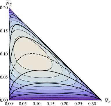
Figure 4: Entropy per disk, $\bar{S}/k_{B}$, versus population densities $\bar{N}_{2^{\prime\prime}},\bar{N}_{2^{\prime}}$ of particles from the two species $2^{\prime\prime}$ and $2^{\prime}$. The contours are at $0.028\ell,\ell=1,\ldots,9$. The solid and dashed curves represent (36) for $\Phi=0,\pm 1.5,\pm 3.0,\pm 5.0$ in ascending order from top to bottom.

In macrostates pertaining to $\Phi=0$, particles 2 form random clusters. They are the states of highest entropy at given $\bar{N}_{2^{\prime}}+\bar{N}_{2^{\prime\prime}}$, represented by the dashed curve in Fig. 4. This particular mix of hosts and tags,

$$\bar{N}_{2^{\prime}}=\frac{1}{4}\left[\sqrt{\bar{N}_{2^{\prime\prime}}(8+\bar{N}_{2^{\prime\prime}})}-5\bar{N}_{2^{\prime\prime}}\right],$$ (37)

produces a characteristic texture of heterogeneity in mass density. Critical macrostates on either side of the dashed curve have mass heterogeneities with textures that reflect a higher degree of ordering.

In macrostates generated on pathways with $\Phi>0$ tags are more abundant and hosts less abundant than in a mixture of randomly placed particles 2. The bottom three solid curves are critical population densities (36) at fixed $\Phi>0$. Clusters of hosts with tags are domains of uniform, low mass density, phase separated from domains of uniform, high mass density. The latter are clusters of tiles v.

These domains suppress the entropy significantly relative to the entropy of random clusters of particles 2. The entropy reduction is evident in the contours of Fig 4 and, more compellingly, in the configurational entropy curves, $\bar{S}(\bar{V})$, shown in Fig. 5(a). The effect is most significant at intermediate volume where large clusters of tiles 2 or tiles v are least likely to be realized by chance.

Figure 5: Entropy per disk versus excess volume at criticality. The five curves, inferred from (35), represent, from top to bottom, critical macrostates characterized (a) by $\Phi=0,1.5,3,5,10$. and (b) by $\Phi=0,-1.5,-3,-5,-10$

A different ordering tendency is manifest in critical macrostates generated along pathways with $\Phi<0$. More hosts and fewer tags are present than in a randomly placed mixture. Critical population densities (36) at fixed $\Phi<0$ are represented by the top three solid curves in Fig. 4. These macrostates exhibit various degrees of dispersal of particles 2. The dispersal flattens out heterogeneities in mass density and thus reduces the entropy.

This ordering tendency manifests itself differently in the configurational entropy as shown in Fig. 5(b). Dispersal of particles 2 only produces ordering tendencies in conjunction with spatial constraints. The entropy reduction remains insignificant until crowding of particles 2 becomes an issue. The capacity of the channel for hosts $\mathsf{2^{\prime}}$ is only 60% of its capacity for particles 2. Hence, hosts alone reach saturation at $\bar{V}/q\sigma=\frac{1}{5}$ in an ordered state. At larger $\bar{V}$, the entropy rises again on account of tags attached to some hosts.

6 Friction

The assumption of frictionless surfaces puts some distance between physical reality and the results presented thus far. Here we narrow that gap somewhat. Friction will stabilize additional configurations of jammed disks. However, a rigorous analysis in the framework of configurational statistics now appears remote. The jammed microstates are no longer countable. They include configurations with disks that do not touch any wall. Friction allows a disk to be wedged in between two disks that touch the same wall. The range of distance between the middle disk and the wall depends on the coefficient of friction.

It appears reasonable to argue that the dominant effect of friction is well represented if we allow the controlled presence of adjacent disks that touch the same wall. Our method is readily adaptable to accommodate this scenario. We extend the set of statistically interacting particles from two species (Table 1) to four species (Table 3). Any tile 1 that is stable in the absence of friction remains a particle of species 1. Any tile 1 that directly follows another tile 1 can only be stabilized by friction. We name it a particle 4. Likewise, in any string of adjacent tiles 2, the first is a particle 2 and the others are particles 3.

Table 3: Specifications of four species of particles: species, volume and energy (relative to vacuum), capacity constant (left), and statistical interaction coefficients (right).

• $m$	$v_{m}$	$\epsilon_{m}$	$A_{m}$
  $1$	$q\sigma$	$pq\sigma+\gamma$	$\frac{1}{2}(N-3)$
  $4$	$q\sigma$	$pq\sigma+\gamma+\psi$	$0$
  $2$	$q\sigma$	$pq\sigma-\gamma$	$\frac{1}{2}(N-3)$
  $3$	$q\sigma$	$pq\sigma-\gamma+\psi$	$0$

  $g_{mm^{\prime}}$	$1$	$4$	$2$	$3$
  $1$	$\frac{3}{2}$	$\frac{1}{2}$	$\frac{1}{2}$	$\frac{1}{2}$
  $4$	$-1$	$0$	$0$	$0$
  $2$	$\frac{1}{2}$	$\frac{1}{2}$	$\frac{3}{2}$	$\frac{1}{2}$
  $3$	$0$	$0$	$-1$	$0$

All four species of particles extend the volume by the same amount $q\sigma$. Their expansion work is identical. The gravitational potential energy is raised (lowered) by $\gamma$ when a particle 1 or 4 (2 or 3) is activated. The population densities of particles 4 and 3 relative to those of particles 1 and 2, respectively, are controllable by the parameter $\psi$ in a role akin to a chemical potential. Unlike $pq\sigma$ in (4) and $\gamma$ in (5), the parameter $\psi$ is not associated with any physically relevant unit of energy. However, its value is determined, via $R_{f}$, by an observable effect of friction. In the taxonomy of Ref. [21] particle 1 is host to tag particle 4 and particle 2 host to tag 3.

Equations (14) for the two pairs of hosts and tags become

$$e^{2K_{p}}=\frac{w_{1}^{2}w_{2}^{2}(1+w_{3})(1+w_{4})}{(1+w_{1})(1+w_{2})w_{3}w_{4}},$$

$$e^{2K_{g}}=\frac{w_{1}w_{3}(1+w_{4})}{w_{2}(1+w_{3})w_{4}},\quad e^{\Psi}=\frac{w_{4}}{w_{1}}=\frac{w_{3}}{w_{2}},$$ (38)

where $\Psi\doteq\psi/T_{k}$. The particle population densities inferred from (15) are

$$\bar{N}_{4}=\frac{\bar{N}_{1}}{w_{4}}=\frac{(1+w_{2})w_{3}}{D^{(\psi)}},\quad\bar{N}_{3}=\frac{\bar{N}_{2}}{w_{3}}=\frac{(1+w_{1})w_{4}}{D^{(\psi)}},$$ (39)

$$D^{(\psi)}=(1+w_{2})w_{3}+(1+w_{1})w_{4}+w_{3}w_{4}[2w_{1}w_{2}+3(w_{1}+w_{2})+4].$$

In the limit $\psi\to\infty$ we have $w_{3},w_{4}\to\infty$ and expressions (20), (21) for the frictionless case are recovered.

Within the limitations of our approach, the effects of friction are most transparently accounted for if we impose the constraints

$$\frac{\bar{N}_{4}}{\bar{N}_{1}}=\frac{\bar{N}_{3}}{\bar{N}_{2}}=R_{f},$$ (40)

because friction is the same near both walls. The parameter $R_{f}$ with range $0\leq R_{f}\leq 1$ is a measure for the coefficient of friction. This simple model to include friction can be modified in the light of evidence from experiments or simulations. We could prohibit, for example, the occurrence of more than three tiles 1 or three tiles 2 adjacent to each other. Within the limitations of this model we can state that $R_{f}$ is zero in the absence of friction and that it increases monotonically with the coefficient of static friction. The asymmetry in Eq. (40) is due to gravity, $\bar{N}_{4}<\bar{N}_{3}$ follows from $\bar{N}_{1}<\bar{N}_{2}$.

The four Eqs. (6) are thus reduced to a pair,

$$\frac{e^{2K_{p}}}{(1+R_{f})^{2}}=\frac{w_{1}^{2}w_{2}^{2}}{(1+w_{1})(1+w_{2})},\quad e^{2K_{g}}=\frac{w_{1}}{w_{2}}.$$ (41)

Expressions (39) for the particle population densities remain intact.

How do the additional tiles stabilized by friction, i.e. the tag particles 3 and 4, affect the configurational entropy curves $\bar{S}(\bar{V})$? The answer is shown in Fig. 6 for $R_{f}=0.1$. In this case we have one tile 1 (2) stabilized by friction for every ten tiles 1 (2) that are stable under pressure and gravity alone.

All features except one are qualitatively the same as in Fig. 3 for the frictionless case. The curves fan out from the most disordered state in a similar manner. Criticality is robust. The coordinates of three landmarks (critical point, points of maximum and minimum volume) have shifted somewhat. The jammed macrostate with maximum volume now has a nonzero entropy. The source of this entropy are the extra tiles stabilized by friction. They are randomly distributed as tags 3 to hosts 2. Tiles 1 are absent from this macrostate.

Figure 6: Entropy per disk versus excess volume at $\Gamma=0,0.5,0.75,1,1.25,1.5,3$ (left to right) with effects of friction included $(R_{f}=0.1)$. The dashed arch delimits a region of critical macrostates.

The critical states, located on the dashed curve in Fig. 6, are again associated with the combined limit (22). Equation (28) for $w_{2}$ remains valid if we divide the left-hand side by $(1+R_{f})^{2}$. The critical particle population densities in the presence of friction are

$$\bar{N}_{1}=\bar{N}_{4}=0,\quad\bar{N}_{2}=\frac{\bar{N}_{3}}{R_{f}}=\frac{1}{R_{f}+3+2w_{2}}.$$ (42)

7 Conclusions

7.1 Analogies

It is interesting to compare the results of this work with the results compiled in [25, 26, 27, 28, 29, 30] for hard sphere subject to friction. There exists a remarkable analogy with similar and contrasting features between jammed macrostates of disks at criticality along the dashed arc of our Fig. 3 and of spheres in the RCP limit along the vertical borderline of the phase diagram in [25]. In both systems the jammed macrostates depend on the compactivity and one additional control parameter, contributed by gravity in our system and by friction in the hard-sphere system.

Approaching our critical line via the limit (22) with a specific value for $\Delta$ in (27) corresponds to approaching the RCP line from the left via the limit $X\to 0$ for a specific value of $\mu$ (coefficient of friction) or $Z$ (mechanical coordination number). The jammed macrostates to the right of the RCP line are shown in [28] to consist of coexisting domains of RCP disorder and FCC order. The RCP line can thus be interpreted as the location of a first-order phase-transition.

In Sec. 5 of this work we show indirect evidence that the macrostates below the (dashed) critical line (see Fig. 5) also consist of coexisting domains of order and disorder. In our case two distinct types of ordering are explored. However, we have yet to develop the mathematical tools for a more direct and quantitative description of the ordered domains.

There exists a second analogy between the two systems. It pertains to the (averaged) mechanical coordination number $Z$. In the hard-sphere system, there appears to exist a function $Z(\mu)$, which was shown to vary monotonically between a low-friction plateau, $Z=6$ and a high-friction plateau, $Z=4$, for jammed macrostates between the RLP and RCP lines [29].

The confined disks of our system have $Z=3$ with no variation in the absence of friction. In Sec. 6 we argue that friction stabilizes additional disk configurations involving disks with only two loaded contacts. Our argument implies that $Z$ decreases monotonically with increasing coefficient of friction. A more quantitative analysis of that functional relation and its dependence on $\bar{V}$ will have to await an analysis based on refined mathematical tools.

7.2 Discussion

The methodology of this work builds on the foundations of configurational statistics. Chief among the assumptions is the existence of jammed macrostates that are systematically reproducible by some protocol of random agitations of given intensity and that can be described by few control variables.

Jammed macrostates of the system under investigation here are parametrized by two variables reflecting the intensity of the random agitations in two distinct energy units of relevance. One unit represents the expansion work of the piston when it is moved a fraction of one disk diameter. The other unit represents the weight of one disk lifted across the channel.

A protocol of random agitations that fits the bill of configurational statistics for the jammed disks in the narrow channel is not guaranteed to exist. If it does exist it may be difficult to implement. It is no secret that this is the Achilles’ heel of configurational statistics.

The detailed predictions of this work follow rigorously from the assumptions underlying configurational statistics if friction is absent. The versatility of our method of analysis makes it possible to include some dominant effects of friction in a transparent way. Our results thus present a situation where the assumptions of configurational statistics can be put to the test of simulations and experiments. The simplicity of the model in conjunction with the complexity of its behavior is well suited for that purpose. Any instances of verification or falsification will shed light on the important question of how accurately a protocol of random agitations applied to jammed granular matter can mimic effects of thermal fluctuations.

7.3 Outlook

Experimental, theoretical, and computational studies of jammed disks are well established [31, 32, 33, 34] but scenarios with highly confined geometries have drawn limited attention thus far [13, 14, 15]. We hope to have shown in this work that such simple systems exhibit behavior that is worth studying for at least two reasons: there exist compelling analogies to behavior of more complex systems, exact analytic results are within reach.

The methodology as presented here is amenable to further development in several directions: (i) the regime $1+\sqrt{3/4}<H/\sigma<2$ of 32 tiles as identified in [14], (ii) mixtures of disks with different radii and masses including rattlers [35, 36, 37], (iii) spatial correlations of heterogeneities in mass density, and (iv) channels with the axis oriented vertically.

References

References

- [1] H. M. Jaeger, S. R. Nagel, and R. P. Behringer, Rev. Mod. Phys. 68, 1259 (1996).
- [2] P. G. de Gennes, Rev. Mod. Phys. 71, S374 (1999).
- [3] E. R. Nowak, J. B. Knight, E. Ben-Naim, H. M. Jaeger, and S. R. Nagel, Phys. Rev. E 57, 1971 (1998).
- [4] N. Xu, Front. Phys. 6, 109 (2011).
- [5] S. F. Edwards and R. B. S. Oakeshott, Physica 157, 1080 (1989).
- [6] A. Mehta and S. F. Edwards, Physica A 157, 1091 (1989).
- [7] S. F. Edwards and C. C. Mounfield, Physica A 210, 290 (1994).
- [8] P. Bak, C. Tang, and K. Wiesenfeld, Phys. Rev. A 38, 364 (1988).
- [9] C. O’Hern, S. A. Langer, A. J. Liu, and S. R. Nagel, Phys. Rev. Lett. 88, 075507 (2002).
- [10] T. S. Majumdar, M. Sperl, S. Luding, and R. P. Behringer, Phys. Rev. Lett. 98, 058001 (2007).
- [11] D. A. Head, Phys. Rev. Lett. 102, 138001 (2009).
- [12] M. Schröter, S. Nägle, C. Radin, and H. L. Swinney, EPL, 78, 44004 (2007).
- [13] R. K. Bowles and I. Saika-Voivod, Phys. Rev. E 73, 011503 (2006).
- [14] S. S. Ashwin and R. K. Bowles, Phys. Rev. Lett. 102, 235701 (2009).
- [15] R. K. Bowles and S. S. Ashwin, arXiv:1102.0352.
- [16] F. D. M. Haldane, Phys. Rev. Lett. 67, 937 (1991).
- [17] Y.-S. Wu, Phys. Rev. Lett. 73, 922 (1994).
- [18] S. B. Isakov, Phys. Rev. Lett. 73, 2150 (1994); Mod. Phys. Lett. B 8, 319 (1994).
- [19] D.-V. Anghel, J. Phys. A 40, F1013 (2007); Europhys. Lett. 87, 60009 (2009).
- [20] P. Lu, J. Vanasse, C. Piecuch, M. Karbach, and G. Müller, J. Phys. A 41, 265003 (2008).
- [21] D. Liu, P. Lu, G. Müller, and M. Karbach, Phys. Rev. E 84, 021136 (2011).
- [22] P. Lu, D. Liu, G. Müller, and M. Karbach Condens. Matter Phys. 15, 13001 (2012).
- [23] D. Liu, J. Vanasse, G. Müller, and M. Karbach, Phys. Rev. E 85, 011144 (2012).
- [24] P. Charbonneau, E. I. Corwin, G. Parisi, and F. Zamponi, Phys. Rev. Lett. 109, 205501 (2012).
- [25] C. Song, P. Wang, and H. A. Makse, Nature 453, 625 (2008).
- [26] C. Briscoe, C. Song, P. Wang, and H. A. Makse, Phys. Rev. Lett. 101, 188001 (2008).
- [27] C. Briscoe, C. Song, P, Wang, and H. A. Makse, Physica A 389, 3978 (2010).
- [28] Y. Jin and H. A. Makse, Physica A 389, 5362 (2010).
- [29] P. Wang, C. Song, Y. Jin, and H. A. Makse, arXiv:0808.2196.
- [30] M. P. Ciamarra, R. Pastore, M. Nicodemi, and A. Coniglio, Phys. Rev. E 84, 041308 (2011).
- [31] S. Meyer, C. Song, Y. Jin, K. Wang, and H. A. Makse, Physica A 389, 5137 (2010).
- [32] B. D. Lubachevsky and F. H. Stillinger, J. Stat. Phys. 60, 561 (1990).
- [33] T. Unger, J. Kertesz, and D. E. Wolf, Phys. Rev. Lett. 94, 178001 (2005).
- [34] J. Zhang, T. S. Majumdar, M. Sperl, and R. P. Behringer, Soft Matter 6, 2982 (2010).
- [35] K. W. Desmond nad E. R. Weeks, Phys. Rev. E 80, 051305 (2009).
- [36] G.-J. Gao, J. Blawzdziewicz, C. S. O’Hern, and M. Shattuck, Phys. Rev. E 80, 061304 (2009).
- [37] S. S. Ashwin, J. Blawzdziewicz, C. S. O’Hern, and M. D. Shattuck, Phys. Rev. E 85, 061307 (2012).