Quantum interference induced by initial system-environment correlations

Abstract

We investigate the quantum interference induced by a relative phase in the correlated initial state of a system which consists in a two-level atom interacting with a damped mode of the radiation field. We show that the initial relative phase has significant effects on both the evolution of the atomic excited-state population and the information flow between the atom and the reservoir, as quantified by the trace distance. Furthermore, by considering two two-level atoms interacting with a common damped mode of the radiation field, we highlight how initial relative phases can affect the subsequent entanglement dynamics.

1 Introduction

Understanding of the time-evolution of open systems is of great relevance not only in the foundations of quantum mechanics, but also in the rapidly developing quantum technologies [1, 2]. In most cases, the initial state of the open system is assumed uncorrelated from its environment, so that the evolution of the open system can be described by a family of completely positive trace preserving (CPT) reduced dynamical maps. Nevertheless, in many concrete experimental situations the investigated system is unavoidably correlated with the environment also at the initial time, especially in the case of systems which are strongly coupled to the reservoir. Therefore, initial correlations between the system and the reservoir represent a fundamental issue, both from a theoretical and an experimental point of view [3, 4, 5, 6, 7, 8, 9, 10, 11, 12, 13]. In particular, if there are initial correlations between an open system and the corresponding environment, the trace distance of two states of the open system can grow over its initial value during the time-evolution [14, 15, 16], indicating that the open system can access some information which is initially outside it. Recently, the trace-distance growth of open-system states above its initial value has been experimentally verified by means of all-optical apparata, in which the system under investigation consists of single photons emitted by quantum dots or couples of entangled photons generated by parametric down conversion [17].

In this paper, we focus on a general effect induced by initial system-environment correlations in the subsequent open-system dynamics. Namely, we show that the quantum interference due to a relative phase in the correlated initial total state plays an important role in several aspects of the dynamics of the open system. In particular, we investigate a system composed of a two-level atom interacting with a mode of the radiation field, which is in turn coupled to a damping reservoir. First, we study the dynamics of atomic excited-state population, thus showing how the quantum interference can modify in different ways the system’s energy gain from the reservoir. Then, we take into account the evolution of the trace distance between atomic states, characterizing the information flow between the atom and the reservoir. It is shown that the initial relative phase plays a basic role in order to maximize the increase of the trace distance above its initial value, i.e., the amount of information that flows from the environment to the open system in the course of the dynamics. Finally, we generalize our model, by taking into account two two-level atoms interacting with a common damped mode of the radiation field. We study how relative phases in a correlated initial atom-mode state influence the dynamics of atomic entanglement, and in particular the steady-state entanglement.

2 Model and solution

In this paper, we consider the damped Jaynes-Cummings model [1], namely a two level atom interacting via the Jaynes-Cummings Hamiltonian with a mode of the radiation field, that is in turn coupled to a damping reservoir. Our aim is to investigate how initial correlations between the atom and the mode influence the subsequent dynamics of the atom and, in particular, we focus on the role of the relative phase in the correlated initial state. Thus, we are not assuming an initial vacuum state of the mode. In the following, we will use the Lindblad master equation for the atom-mode system given by [18]

$$\frac{d\rho(t)}{dt}=-i[H,\rho(t)]-\frac{\Gamma}{2}[b^{+}b\rho(t)-2b\rho(t)b^{+}+\rho(t)b^{+}b],$$ (1)

with $H=\omega_{0}{\sigma}_{+}{\sigma}_{-}+\omega_{c}{b}^{+}{b}+\Omega({\sigma}_{-}{b}^{+}+{\sigma}_{+}{b}),$ where $\rho$ represents the density matrix of the system formed by the atom and the mode, ${\sigma}_{\pm}$ are the raising and lowering operators and $\omega_{0}$ is the transition frequency of the atom. Moreover, $b$ ($b^{\dagger}$) is the annihilation (creation) operator of the mode, with frequency $\omega_{c}$, $\Omega$ is the coupling constant between the atom and the mode, and, finally, $\Gamma$ is the damping rate of the mode due to its interaction with the dissipative reservoir. We focus on the resonant case, i.e. $\omega_{0}=\omega_{c}\equiv\omega$. Note that this master equation, often introduced on the basis of a phenomenological approach, can be microscopically justified for a zero temperature flat reservoir [19] relying on the Born-Markov approximation [1]. It then provides a description of the atom-mode dynamics on a coarse grained time scale, which does not resolve the decay time of correlation functions of the damping reservoir. Finally, let us introduce the basis $|\alpha\rangle_{A}\otimes|n\rangle_{M}\equiv|\alpha,n\rangle_{AM}$, with $\alpha=e,g$ labeling the states of the two-level atom, and $n=0,1,2,\ldots$ the number states of the field mode.

In the following, we first take into account a correlated initial atom-mode pure state $\rho_{AM}^{(1)}(0)=\left|\Psi(0)\right\rangle_{AM}\left\langle\Psi(0)\right|$, with

$$\left|\Psi(0)\right\rangle_{AM}=C_{1}(0)\left|e,0\right\rangle_{AM}+C_{2}(0)\left|g,1\right\rangle_{AM}.$$ (2)

The reduced states of the atom and the mode are, respectively, $\rho_{A}^{(1)}(0)=|C_{1}(0)|^{2}\left|e\right\rangle\left\langle e\right|+|C_{2}(0)|^{2}\left|g\right\rangle\left\langle g\right|$ and $\rho_{M}^{(1)}(0)=|C_{1}(0)|^{2}\left|0\right\rangle\left\langle 0\right|+|C_{2}(0)|^{2}\left|1\right\rangle\left\langle 1\right|$. To make a comparison with the uncorrelated situation, we then consider a product initial atom-mode state in the form

$$\rho_{AM}^{(2)}(0)=\rho_{A}^{(2)}(0)\otimes\rho_{M}^{(2)}(0),$$ (3)

with $\rho_{A}^{(2)}(0)=|B_{1}(0)|^{2}\left|e\right\rangle\left\langle e\right|+|B_{2}(0)|^{2}\left|g\right\rangle\left\langle g\right|$ and $\rho_{M}^{(2)}(0)=\rho_{M}^{(1)}(0)$. Note that the initial atom-mode states $\rho_{AM}^{(1)}(0)$ and $\rho_{AM}^{(2)}(0)$ have the same reduced states for the mode, but they may have different reduced states for the atom.

Now, consider the correlated initial state $\rho_{AM}^{(1)}(0)$. Since there is only one excitation in the total system, we can make the ansatz that the atom-mode state at time $t$ is of the form [20, 21]

$$\rho^{(1)}_{AM}(t)=(1-\lambda(t))|\psi(t)\rangle_{AM}\langle\psi(t)|+\lambda(t)|g,0\rangle_{AM}\langle g,0|,$$ (4)

with $0\leq\lambda(t)\leq 1$, $\lambda(0)=0$, and $|\psi(t)\rangle_{AM}=C_{1}(t)|e,0\rangle_{AM}+C_{2}(t)|g,1\rangle_{AM}.$ In the spirit of [20], it is convenient to introduce the unnormalized state vector

$$|\widetilde{\psi}(t)\rangle_{AM}\equiv{\sqrt{(1-\lambda(t))}}|\psi(t)\rangle_{AM}=\widetilde{C}_{1}(t)|e,0\rangle_{AM}+\widetilde{C}_{2}(t)|g,1\rangle_{AM},$$ (5)

where $\widetilde{C}_{k}(t)\equiv{\sqrt{(1-\lambda(t))}}C_{k}(t)$, for $k=1,2$, and therefore the atom-mode state at time $t$ can be written as $\rho^{(1)}_{AM}(t)=|\widetilde{\psi}(t)\rangle_{AM}\langle\widetilde{\psi}(t)|+\lambda(t)|g,0\rangle_{AM}\langle g,0|$. Due to Eq.(1) the dynamics of the unnormalized atom-mode state in Eq. (5) is determined by [20]:

$$i\frac{d}{dt}\widetilde{C}_{1}(t) = \omega\widetilde{C}_{1}(t)+\Omega\widetilde{C}_{2}(t),$$

$$i\frac{d}{dt}\widetilde{C}_{2}(t) = \left(\omega-i\frac{\Gamma}{2}\right)\widetilde{C}_{2}(t)+\Omega\widetilde{C}_{1}(t),$$ (6)

while $\lambda(t)$ satisfies $d\lambda(t)/dt=\Gamma|\widetilde{C}_{2}(t)|^{2}$. By means of the Laplace transformation, together with the initial condition $\left|\Psi(0)\right\rangle_{AM}$ given by Eq. (2), we get the analytical expression $\widetilde{C}_{1}(t)=\mu(t)C_{1}(0)-i\nu(t)C_{2}(0)$, with

$$\mu(t) = e^{-(\frac{\Gamma}{4}+i\omega)t}\left[\cosh(\frac{at}{2})+\frac{\Gamma}{2a}\sinh(\frac{at}{2})\right],$$ (7)

$$\nu(t) = e^{-(\frac{\Gamma}{4}+i\omega)t}\left[\frac{2\Omega}{a}\sinh(\frac{at}{2})\right],$$ (8)

and $a=\sqrt{(\Gamma/2)^{2}-4\Omega^{2}}$. One may distinguish two different dynamical regimes via $\Gamma$ and $\Omega$; namely, we will identify the case $\Gamma>2\Omega$ as the weak coupling regime and $\Gamma<2\Omega$ as the strong coupling regime [21]. From Eqs. (4) and (5), one has that the reduced state of the atom at time $t>0$ can be expressed as

$$\rho_{A}^{(1)}(t)=|C_{e}^{(1)}(t)|^{2}\left|e\right\rangle\left\langle e\right|+(1-|C_{e}^{(1)}(t)|^{2})\left|g\right\rangle\left\langle g\right|,$$ (9)

with $|C_{e}^{(1)}(t)|^{2}\equiv|\widetilde{C}_{1}(t)|^{2}$.

Let us now take into account the uncorrelated initial atom-mode state $\rho_{AM}^{(2)}(0)$. It can be written as the mixture of four pure states, i.e., $\left|e,0\right\rangle\left\langle e,0\right|$, $\left|g,1\right\rangle\left\langle g,1\right|$, $\left|e,1\right\rangle\left\langle e,1\right|$ and $\left|g,0\right\rangle\left\langle g,0\right|$. For later convenience, we separately evaluate the different contributions given by these four terms to the probability of the atom being in excited state at a time $t$. By the previous analysis, it is clear that the contributions due to $\left|e,0\right\rangle\left\langle e,0\right|$ and $\left|g,1\right\rangle\left\langle g,1\right|$ are just, respectively, $|\mu(t)|^{2}$ and $|\nu(t)|^{2}$, see Eqs.(7) and (8). The term $\left|g,0\right\rangle\left\langle g,0\right|$ is invariant, while for the contribution of $\left|e,1\right\rangle\left\langle e,1\right|$ we have to come back to the master equation (1) and set the initial condition $\rho(0)=|e,1\rangle\langle e,1|$, thus getting the system of equations:

$$\dot{\varrho}_{11}(t) = -i[\sqrt{2}\varrho_{21}(t)\Omega-\sqrt{2}\varrho_{12}(t)\Omega]-\Gamma\varrho_{11}(t)$$

$$\dot{\varrho}_{12}(t) = -i[\varrho_{12}(t)\omega_{0}-\varrho_{12}(t)\omega_{c}+\sqrt{2}\varrho_{22}(t)\Omega-\sqrt{2}\varrho_{11}(t)\Omega]-\frac{3\Gamma}{2}\varrho_{12}(t)$$

$$\dot{\varrho}_{22}(t) = -i[\sqrt{2}\varrho_{12}(t)\Omega-\sqrt{2}\varrho_{21}(t)\Omega]-2\Gamma\varrho_{22}(t)$$

$$\dot{\varrho}_{33}(t) = -i[\varrho_{43}(t)\Omega-\varrho_{34}(t)\Omega]+\Gamma\varrho_{11}(t)$$

$$\dot{\varrho}_{34}(t) = -i[\varrho_{34}(t)\omega_{0}+\varrho_{44}(t)\Omega-\varrho_{34}(t)\omega_{c}-\varrho_{33}(t)\Omega]-\frac{\Gamma}{2}[\varrho_{34}(t)-2\sqrt{2}\varrho_{12}(t)]$$

$$\dot{\varrho}_{44}(t) = -i[\varrho_{44}(t)\omega_{c}+\varrho_{34}(t)\Omega-\varrho_{43}(t)\Omega]-\frac{\Gamma}{2}[2\varrho_{44}(t)-4\varrho_{22}(t)].$$ (10)

We indicated the atom-mode state at time $t$ as $\varrho(t)$ to emphasize that it corresponds to the specific above-mentioned initial condition, and the matrix elements of $\varrho(t)$ are expressed with respect to the atom-mode states $\{\left|\widetilde{0}\right\rangle=\left|g,0\right\rangle,\left|\widetilde{1}\right\rangle=\left|e,1\right\rangle,\left|\widetilde{2}\right\rangle=\left|g,2\right\rangle,\left|\widetilde{3}\right\rangle=\left|e,0\right\rangle,\left|\widetilde{4}\right\rangle=\left|g,1\right\rangle\}$, with the notation $\varrho_{kl}(t)\equiv\left\langle\widetilde{k}\right|\varrho(t)\left|\widetilde{l}\right\rangle$. By solving these equations, we get the probability $\varrho_{11}(t)+\varrho_{33}(t)$ for atomic excited-state occupation induced by the term $\left|e,1\right\rangle\left\langle e,1\right|$. Summarizing, the reduced state of the atom at time $t>0$ for the initial atom-mode state $\rho_{AM}^{(2)}(0)$ reads $\rho_{A}^{(2)}(t)=|C_{e}^{(2)}(t)|^{2}\left|e\right\rangle\left\langle e\right|+(1-|C_{e}^{(2)}(t)|^{2})\left|g\right\rangle\left\langle g\right|$ with

$$|C_{e}^{(2)}(t)|^{2}=|B_{1}(0)C_{1}(0)\mu(t)|^{2}+|B_{2}(0)C_{2}(0)\nu(t)|^{2}+|B_{1}(0)C_{2}(0)|^{2}[\varrho_{11}(t)+\varrho_{33}(t)].$$ (11)

3 Dynamics of atomic excited-state population

In this work, we are concerned with the specific effects of initial atom-mode correlations on atomic dynamics and, in particular, we stress the role of the relative phase in the correlated initial atom-mode state. Thus, let us reexpress $C_{1}(0)$ and $C_{2}(0)$ in Eq. (2) as $C_{1}(0)=\mathcal{C}_{1}(0)$ and $C_{2}(0)=\mathcal{C}_{2}(0)e^{i\theta},$ where $\mathcal{C}_{1}(0)$ and $\mathcal{C}_{2}(0)$ are real numbers and $\theta\in[0,2\pi]$. For the correlated initial state, the atomic excited-state population is given by, see Eq. (9),

$$|C_{e}^{(1)}(t)|^{2}=|\mu(t)|^{2}\mathcal{C}_{1}^{2}(0)+|\nu(t)|^{2}\mathcal{C}_{2}^{2}(0)+2\mu(t)\nu^{*}(t)\mathcal{C}_{1}(0)\mathcal{C}_{2}(0)\sin\theta,$$ (12)

with $\mu(t)$ and $\nu(t)$ as in Eqs. (7) and (8), respectively. The first term represents the transfer of excitation that is initially in the atom with probability $\mathcal{C}_{1}^{2}(0)$, while the second term represents the transfer of excitation that is initially in the mode with probability $\mathcal{C}_{2}^{2}(0)$. These two processes coexist in the whole course of evolution and, indeed, quantum interference can be induced between them, which is just denoted by the third term in Eq. (12). Obviously, the constructive (destructive) quantum interference corresponds to $\theta\in(0,\pi)$ ($\theta\in(\pi,2\pi)$), while for $\theta=0,\pi,2\pi$ there is no quantum interference. For convenience, we define a rescaled probability of the atomic excited-state population as $\tilde{P}_{e}(t)=|C_{e}^{(k)}(t)/C_{e}^{(k)}(0)|^{2},$ where $k=1,2$ refer to, respectively, the initially correlated and uncorrelated states of the total system.

First, we consider the case without quantum interference. The uncorrelated initial state $\rho_{AM}^{(2)}(0)$ in Eq. (3) is chosen as the tensor product of the marginals of the correlated state $\rho_{AM}^{(1)}(0)$, so that the probability of atomic excited-state occupation is obtained by putting $B_{1}(0)=\mathcal{C}_{1}(0)$ and $B_{2}(0)=\mathcal{C}_{2}(0)$ into Eq.(11). In Fig.1 (a) and (b), we plot the time-evolution of the rescaled probability of the atomic excited-state population $\tilde{P}_{e}(t)$ for the initial states $\rho_{AM}^{(1)}(0)$ (solid lines) and $\rho_{AM}^{(2)}(0)$ (dashed lines) and for different values of $\mathcal{C}_{1}(0)$ and $\mathcal{C}_{2}(0$). In both weak and strong coupling regimes and for both initially correlated and uncorrelated situations, $\tilde{P}_{e}(t)>1$ occurs when $\mathcal{C}_{2}(0)>\mathcal{C}_{1}(0)$. We observe that the amplitude of the increase of $\tilde{P}_{e}(t)$ from the initial value one in the presence of initial correlations is always larger than that without initial correlations. Moreover, for $\mathcal{C}_{2}(0)\leq\mathcal{C}_{1}(0)$ one can see that $\tilde{P}_{e}(t)$ in the presence of initial correlations is still larger than without initial correlations (the inset in Fig.1 (a) shows an enlarged figure). Initial correlations in the absence of interference can be identified as a mechanism that increases the excitation transfer from the mode to the atom and inhibit the opposite process.

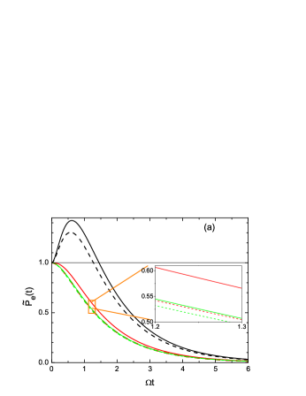
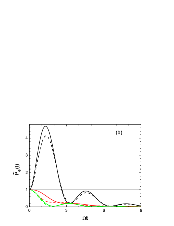
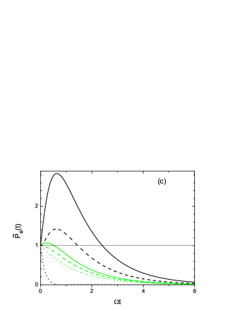
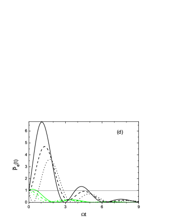
Figure 1: (a,b): Time-evolution of $\tilde{P}_{e}(t)$ for the correlated initial state $\rho_{AM}^{(1)}(0)$ with $\theta=0$ (solid lines) and for the uncorrelated initial state $\rho_{AM}^{(2)}(0)$ (dashed lines) in (a) weak ($\Gamma/\Omega=6$) and (b) strong ($\Gamma/\Omega=1$) coupling regimes. (c,d): Time-evolution of $\tilde{P}_{e}(t)$ for $\rho_{AM}^{(1)}(0)$ under different relative phases in terms of $\theta=\pi/2$ (solid lines), $\theta=0$ (dashed lines) and $\theta=3\pi/2$ (dotted lines) in (c) weak ($\Gamma/\Omega=6$) and (d) strong ($\Gamma/\Omega=1$) coupling regimes. The other parameters are $\mathcal{C}_{1}(0)=\sqrt{\frac{1}{10}}<\mathcal{C}_{2}(0)=\sqrt{\frac{9}{10}}$ (black line); $\mathcal{C}_{1}(0)=\mathcal{C}_{2}(0)=\sqrt{\frac{1}{2}}$ (red line); $\mathcal{C}_{1}(0)=\sqrt{\frac{9}{10}}>\mathcal{C}_{2}(0)=\sqrt{\frac{1}{10}}$ (green line), and $B_{1}(0)=\mathcal{C}_{1}(0)$, $B_{2}(0)=\mathcal{C}_{2}(0)$.

Next, we explore the role of quantum interference in influencing atomic excited-state population. In Fig.1 (c) and (d), we plot the time-evolution of $\tilde{P}_{e}(t)$ for the correlated initial state $\rho_{AM}^{(1)}(0)$ for different values of $\mathcal{C}_{1}(0)$ and $\mathcal{C}_{2}(0)$ and for $\theta=\pi/2$ (solid lines), $\theta=3\pi/2$ (dotted lines) and $\theta=0$ (dashed lines), i.e. for, respectively, constructive, destructive and no quantum interference. Indeed, for the corresponding product state $\rho_{AM}^{(2)}(0)$ the time-evolution of $\tilde{P}_{e}(t)$ is the same in all the different situations. We observe that, in the case of constructive interference, the rescaled probability $\tilde{P}_{e}(t)$ for the correlated initial state always reaches values greater than one, irrespective of the ratio $\mathcal{C}_{2}(0)/\mathcal{C}_{1}(0)$. Moreover, also for $\mathcal{C}_{2}(0)>\mathcal{C}_{1}(0)$ the amplitude growth of $\tilde{P}_{e}(t)$ has largely increased as compared to the case $\theta=0$: the constructive interference boosts the energy flow from the mode to the atom and inhibits the opposite process. On the other hand, for a destructive interference, $\tilde{P}_{e}(t)$ is always lesser than one in the weak coupling regime, irrespective of the ratio $\mathcal{C}_{2}(0)/\mathcal{C}_{1}(0)$ and, besides, the greater this ratio is, the faster the atom decays. In addition, in the strong coupling regime $\tilde{P}_{e}(t)$ decays on short time scales and then, even if it can increase up to values greater than one for $\mathcal{C}_{2}(0)>\mathcal{C}_{1}(0)$ in the later evolution, its maximum value is clearly smaller than that of $\theta=0$ and $\theta=\pi/2$. Therefore, we can conclude that the destructive interference boosts the energy flow from the atom to the mode. Summarizing, as far as the ability to facilitate the energy flow from the mode to the atom and restrain the opposite process is taken into account, initial correlations turn out to be crucial because of interference effects.

4 Dynamics of the trace distance between atomic states

In this section, we investigate the influence of initial correlations and relative phase on the dynamics of the trace distance of atomic states. Trace distance is one of the most employed quantifiers for the distinguishability of quantum states. A change of the trace distance between reduced-system states in the course of the dynamics indicates an information flow between the open system and the environment [22]. The trace distance $D(\rho_{1},\rho_{2})$ between two quantum states $\rho_{1}$ and $\rho_{2}$ is defined as [2] $D(\rho_{1},\rho_{2})=\frac{1}{2}\|\rho_{1}-\rho_{2}\|_{1},$ where $\|X\|_{1}=\mathrm{Tr}\sqrt{X^{{\dagger}}X}$ is the trace norm of the operator $X$. Any positive and trace-preserving map $\mathcal{E}$ defined on the whole space of trace class operators is a contraction for the trace distance, i.e., $D(\mathcal{E}(\rho_{1}),\mathcal{E}(\rho_{2}))\leq D(\rho_{1},\rho_{2})$. In the presence of initial correlations the contractivity may fail since the trace distance $D(\rho^{1}_{S}(t),\rho^{2}_{S}(t))$ between two states of the open system, $\rho^{1}_{S}(t)$ and $\rho^{2}_{S}(t)$ evolved from the initial total states $\rho^{1}_{SE}(0)$ and $\rho^{2}_{SE}(0)$, can exceed its initial value in the course of time-evolution [14]. One can further determine an upper bound to the growth of trace distance, which is $I(\rho_{SE}^{(1)}(0),\rho_{SE}^{(2)}(0))\equiv D(\rho_{SE}^{(1)}(0),\rho_{SE}^{(2)}(0))-D(\rho_{S}^{1}(0),\rho_{S}^{2}(0))$. This quantity can be interpreted as the relative information about the total initial states $\rho_{SE}^{(1)}(0)$ and $\rho_{SE}^{(2)}(0)$ that is initially outside the open system, i.e., that is inaccessible for local measurements performed on the open system only [14].

For the case at hand, the evolution of the total system composed by the atom and the mode is not unitary, but it is given by the family of CPT maps forming the semigroup fixed by Eq. (1). Then, also in this case, from the contractivity of the trace distance, one can immediately see that the increase of the trace distance between atomic states over its initial value is bounded from above by

$$D(\rho_{A}^{(1)}(t),\rho_{A}^{(2)}(t))-D(\rho_{A}^{(1)}(0),\rho_{A}^{(2)}(0))\leq I(\rho_{AM}^{(1)}(0),\rho_{AM}^{(2)}(0)).$$ (13)

For the initial atom-mode states $\rho_{AM}^{(1)}(0)$ given by Eq. (2) and $\rho_{AM}^{(2)}(0)$ as in Eq. (3), the quantity $I(\rho_{AM}^{(1)}(0),\rho_{AM}^{(2)}(0))$ is given by

$$I(\rho_{AM}^{(1)}(0),\rho_{AM}^{(2)}(0))=\frac{1}{2}(\sqrt{(|B_{2}(0)C_{1}(0)|^{2}-|B_{1}(0)C_{2}(0)|^{2})^{2}+4|C_{1}(0)C_{2}(0)|^{2}}$$

$$+|B_{2}(0)C_{1}(0)|^{2}+|B_{1}(0)C_{2}(0)|^{2})-||C_{2}(0)|^{2}-|B_{2}(0)|^{2}|.$$ (14)

When $I(\rho_{AM}^{(1)}(0),\rho_{AM}^{(2)}(0))>0$ the trace distance of atomic states can increase above its initial value in the time-evolution, indicating that the information initially outside the open system is flowing back to it during the dynamics.

The evolution of the trace distance of open system’s states in the presence of initial correlations was investigated in Ref. [16] for a Jaynes-Cummings model without dissipation. Here, we extend the study to the dissipative model, in order to examine the influence of both the dissipation and the relative phase on the dynamics of the trace distance. For the initial atom-mode states $\rho_{AM}^{(1)}(0)$ in Eq. (2) and $\rho_{AM}^{(2)}(0)$ in Eq. (3), the trace distance between the corresponding atomic states at time $t>0$ is simply given by

$$D(\rho_{A}^{(1)}(t),\rho_{A}^{(2)}(t))=||C_{e}^{(1)}(t)|^{2}-|C_{e}^{(2)}(t)|^{2}|.$$ (15)

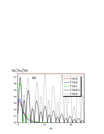
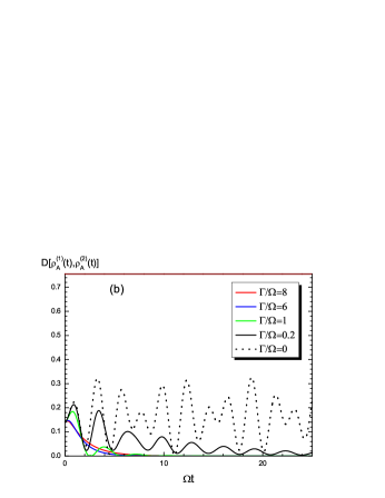
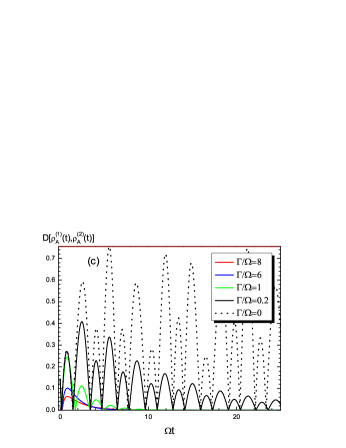
Figure 2: Plot of the trace distance $D(\rho_{A}^{(1)}(t),\rho_{A}^{(2)}(t))$ as a function of rescaled time $\Omega t$. In (a) the parameters characterizing the correlated initial atom-mode state are $C_{1}(0)=\sqrt{\frac{4}{7}}$, $C_{2}(0)=i\sqrt{\frac{3}{7}}$, in (b) $C_{1}(0)=\sqrt{\frac{4}{7}}$, $C_{2}(0)=\sqrt{\frac{3}{7}}$, while in (c) $C_{1}(0)=\sqrt{\frac{4}{7}}$, $C_{2}(0)=-i\sqrt{\frac{3}{7}}$. In all the (a), (b) and (c), the parameters characterizing the initially uncorrelated state of atom-mode are $B_{1}(0)=C_{2}(0)$, $B_{2}(0)=C_{1}(0)$. The top horizontal line in the figures marks the upper bound due to Eq. (4).

In Fig.2 (a), (b) and (c), we plot the dynamics of the trace distance in Eq. (15) without dissipation, i.e., for $\Gamma=0$ and with dissipation for various values of $\Gamma/\Omega$, and we consider, respectively, $\theta=\frac{\pi}{2},0$ and $\frac{3\pi}{2}$ for the correlated initial atom-mode state (2). For the uncorrelated state (3), we set $B_{1}(0)=C_{2}(0)$, $B_{2}(0)=C_{1}(0)$, the same as in [16]. The trace distance of atomic states can exceed its initial value for both $\Gamma=0$ and $\Gamma/\Omega\neq 0$, however only in the former case it can reach the upper bound in Eq. (4) in the course of time, see Fig.2 (a) and (c). In the presence of dissipation, because of the coupling with a larger environment as in Eq. (1), the information flowing from the atom to the mode can flow into the remaining part of the structured reservoir, as well. But then, it can no longer flow back to the atom-mode system since the mode leaks into a Markovian reservoir, i.e., there is a unidirectional flow of information from the mode to the reservoir [22]. The distinct behaviors of the trace distance in weak and strong coupling regimes are exhibited, respectively, by asymptotical decay and damped oscillations.

In Fig.2, one can observe the crucial influence of the initial relative phase on the dynamics of the trace distance between atomic states and, in particular, on the maximum value attained, i.e., the maximum amount of information that is accessible through measurements performed on the open system only [16]. This is the case both for the dissipative situation and for $\Gamma=0$, where the presence of an initial relative phase allows to reach the upper bound in Eq.(4). In the case of a vanishing relative phase, that is shown in Fig.2 (b), the maximum value of the trace distance between atomic states is in fact substantially smaller than the upper bound in Eq. (4), even for $\Gamma=0$. Note that, unlike the excitation transfer described in the previous section, the back flow of information to the atom, which is reflected into the maximum value reached by the trace distance, is strongly amplified by both constructive and destructive interference. Indeed, this traces back to the specific dependence of the information flow between the atom and the mode on the the atomic excited-state populations with and without initial correlations, see Eq. (15). In addition, one can easily find several examples showing how the initial relative phase plays an indispensable role also in determining whether the trace distance of atomic states can actually increase above its initial value, which is indeed a priori not guaranteed by the condition $I[\rho_{AM}^{(1)}(0),\rho_{AM}^{(2)}(0)]>0$.

5 Enhancement of entanglement

In order to give a further evidence of the role of the initial relative phase, we focus now on the dynamics of the entanglement between two atoms interacting with a common structured reservoir. The effect of initial correlations on the entanglement dynamics have been studied in [23, 24].

Consider two identical two-level atoms $A$ and $B$ interacting with a common mode of the radiation field, that is in turn coupled to a damping reservoir. We further assume that the atoms-mode dynamics is determined by the Lindblad equation (1), where $\rho$ now represents the density operator of the system formed by the two atoms and the mode. The Hamiltonian ${H}={H}_{0}+{H}_{\mathrm{int}}+{H}_{dd}$ is given by the sum of the free Hamiltonian, ${H}_{0}=\omega_{0}{\sigma}_{+}^{A}{\sigma}_{-}^{A}+\omega_{0}{\sigma}_{+}^{B}{\sigma}_{-}^{B}+\omega_{c}{b}^{{\dagger}}{b}$, the coupling term between the atoms and the mode ${H}_{\mathrm{int}}=\Omega[({\sigma}_{-}^{A}+{\sigma}_{-}^{B}){b}^{{\dagger}}+({\sigma}_{+}^{A}+{\sigma}_{+}^{B}){b}],$ and the term describing dipole-dipole interaction of the atoms, ${H}_{dd}=D({\sigma}_{+}^{(A)}{\sigma}_{-}^{(B)}+{\sigma}_{-}^{(A)}{\sigma}_{+}^{(B)}).$ Indeed, ${\sigma}_{\pm}^{j}$ ($j=A,B$) are the raising and lowering operators, $\omega_{0}$ is the transition frequency of the atom, $\Omega$ is the coupling constant between the atoms and the mode and $D$ is the coupling strength of the two atoms. Here, we take into account a correlated initial state $\rho_{ABM}(0)=\left|\Psi(0)\right\rangle_{ABM}\left\langle\Psi(0)\right|$, where

$$\left|\Psi(0)\right\rangle_{ABM}=C_{1}(0)\left|e,g,0\right\rangle_{ABM}+C_{2}(0)\left|g,e,0\right\rangle_{ABM}+C_{3}(0)\left|g,g,1\right\rangle_{AM}.$$ (16)

Since there is only one excitation in the total system, we proceed as in Sec.2 and make the ansatz that the atoms-mode state at time $t$ is of the form $\rho_{ABM}(t)=|\tilde{\psi}(t)\rangle_{ABM}\langle\tilde{\psi}(t)|+\lambda(t)|g,g,0\rangle_{ABM}\langle g,g,0|,$ with $0\leq\lambda(t)\leq 1$, $\lambda(0)=0$ and

$$|\widetilde{\psi}(t)\rangle_{ABM}=\widetilde{C}_{1}(t)|e,g,0\rangle_{AM}+\widetilde{C}_{2}(t)|g,e,0\rangle_{ABM}+\widetilde{C}_{3}(t)|g,g,1\rangle_{ABM}.$$ (17)

The dynamics of the unnormalized atoms-mode state in Eq. (17) is fixed by:

$$i\frac{d}{dt}\widetilde{C}_{1}(t) = \omega\widetilde{C}_{1}(t)+\Omega\widetilde{C}_{3}(t)+D\widetilde{C}_{2}(t),$$

$$i\frac{d}{dt}\widetilde{C}_{2}(t) = \omega\widetilde{C}_{2}(t)+\Omega\widetilde{C}_{3}(t)+D\widetilde{C}_{1}(t),$$

$$i\frac{d}{dt}\widetilde{C}_{3}(t) = \left(\omega-i\frac{\Gamma}{2}\right)\widetilde{C}_{3}(t)+\Omega\widetilde{C}_{1}(t)+\Omega\widetilde{C}_{2}(t),$$ (18)

while $\lambda(t)$ satisfies $d\lambda(t)/dt=\Gamma|\widetilde{C}_{3}(t)|^{2}.$ To quantify the entanglement of the two atoms, we adopt Wootters’ concurrence [25], which for any two-qubits density matrix $\rho$ is defined as $C(\rho)=\max\{0,\sqrt{\lambda_{1}}-\sqrt{\lambda_{2}}-\sqrt{\lambda_{3}}-\sqrt{\lambda_{4}}\},$ where $\lambda_{i}$ ($\lambda_{1}\geq\lambda_{2}\geq\lambda_{3}\geq\lambda_{4})$ are the eigenvalues of the matrix $\zeta=\rho(\sigma_{y}\otimes\sigma_{y})\rho^{*}(\sigma_{y}\otimes\sigma_{y}),$ with $\sigma_{y}$ the Pauli matrix and $\rho^{*}$ the complex conjugation of $\rho$ in the standard basis. From Eq (17), one has for the concurrence of atoms $A$ and $B$

$$C_{AB}(t)=2|\widetilde{C}_{1}(t)\widetilde{C}_{2}(t)|.$$ (19)

In the following, we use the notation $C_{1}(0)=\mathcal{C}_{1}(0),C_{2}(0)=\mathcal{C}_{2}(0)e^{i\theta_{1}},C_{3}(0)=\mathcal{C}_{3}(0)e^{i\theta_{2}},$ where $\mathcal{C}_{1}(0)$, $\mathcal{C}_{2}(0)$ and $\mathcal{C}_{3}(0)$ are real numbers and $\theta_{1},\theta_{2}\in[0,2\pi]$.

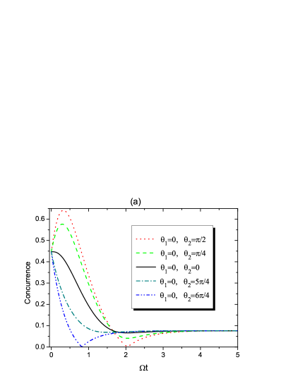
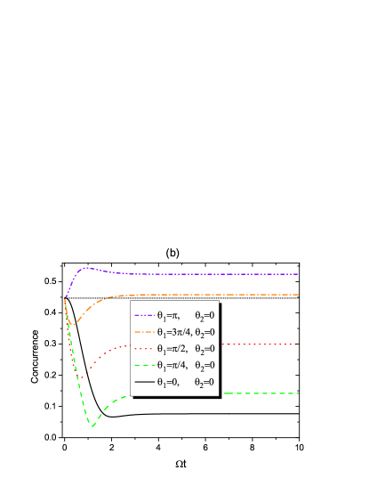
Figure 3: The evolution of the concurrence $C_{AB}(t)$ of atoms $A$ and $B$ for the correlated initial state $\rho_{ABM}(0)$ with various relative phases $\theta_{1}$ and $\theta_{2}$. The solid line is referred to the case with $\theta_{1}=\theta_{2}=0$. The parameters characterizing the initial correlated state are $\mathcal{C}_{1}(0)=\sqrt{\frac{1}{2}}$, $\mathcal{C}_{2}(0)=\sqrt{\frac{1}{10}}$ and $\mathcal{C}_{3}(0)=\sqrt{\frac{4}{10}}$. The other parameters are $\Gamma/\Omega=6$ and $D=0$.

In Fig.3 (a) and (b), we plot the time-evolution of the concurrence $C_{AB}(t)$ for the correlated initial state (16), with various relative phases $\theta_{1}$ and $\theta_{2}$. We set $D=0$ in order to focus on the entanglement dynamics due to the interaction with the environment. Fig.3 (a) shows the variations of $C_{AB}(t)$ for different $\theta_{2}$ with a fixed $\theta_{1}=0$. It is worth noting that the entanglement can exhibit a temporary growth over its initial value, e.g. for $\theta_{2}=\pi/4,\pi/2$, and the amplitude of the growth is determined by $\theta_{2}$. We also note that, though the phase $\theta_{2}$ affects the dynamics of atomic entanglement, the steady entanglement does not depend on it. On the other hand, as shown in Fig.3 (b), steady entanglement can be increased by adjusting the relative phase $\theta_{1}$ with a fixed $\theta_{2}$ and, in particular, it grows through changing the initial phase $\theta_{1}$ from $0$ to $\pi$. Interestingly, the steady entanglement can be greater than the initial entanglement for some values of $\theta_{1}$ (e.g., here $\theta_{1}=3\pi/4,\pi$). Moreover, for $\theta_{1}=\pi$ and $\theta_{2}=0$, atomic entanglement starts increasing at the initial time and then it takes values that are always higher than the initial one. The physical reason for these results can still be attributed to the quantum interference induced by the initial relative phases. The only difference between the present situation and that of a single atom is the increased amount of processes involved in quantum interference.

6 Conclusion

We have investigated the role of the relative phase of a correlated initial total state in the subsequent open-system dynamics. In particular, we have taken into account the dynamics of a two-level atom interacting with a structured reservoir. The initial relative phase affects the two processes of excitation transfer, respectively, from the atom to the mode and from the mode to the atom. We have further shown how this reflects into the dynamics of the information flow between the atom and the reservoir. The quantum interference induced by an initial relative phase, in fact, strongly influences the dynamics of the trace distance of atomic states and in particular the maximum value that it actually reaches during the dynamics. Finally, we have considered two two-level atoms interacting with the same structured reservoir. We have shown how relative phases in the initial correlated total state can enhance atomic entanglement. As a final remark, let us note that the sensitivity of open system dynamics on the initial relative phase suggests possible ways to detect it through measurements on the open system only [17]. The trace-distance analysis of reduced dynamics allows to access, apart from overall correlation properties [22, 26], specific features of the initial total state, which can be useful, e.g., when this is only partially controlled during the preparation procedure.

Acknowledgments

We thank Prof. Masashi Ban for useful comments and suggestions. This work is supported by National Natural Science Foundation of China under Grant Nos. 10947006 and 61178012, the Specialized Research Fund for the Doctoral Program of Higher Education under Grant No. 20093705110001, Scientific Research Foundation of Qufu Normal University for Doctors, MIUR under PRIN 2008, and COST under MP1006.

References

- [1] H.-P. Breuer, F. Petruccione, The Theory of Open Quantum Systems, Oxford University Press, Oxford, 2002.
- [2] M.A. Nielsen, I.L. Chuang, Quantum Computation and Quantum Information, Cambridge University Press, Cambridge, 2000.
- [3] P. Pechukas, Phys. Rev. Lett. 73 (1994) 1060.
- [4] L. D. Romero, J.P. Paz, Phys. Rev. A 55 (1997) 4070.
- [5] P. Štelmachovič, V. Bužek, Phys. Rev. A 64 (2001) 062106.
- [6] T.F. Jordan, A. Shaji, E.C.G. Sudarshan, Phys. Rev. A 70 (2004) 052110.
- [7] M. Ban, Phys. Rev. A 80 (2009) 064103.
- [8] Y. J. Zhang, X. B. Zou, Y. J. Xia, G. C. Guo, Phys. Rev. A 82 (2010) 022108.
- [9] A. G. Dijkstra, Y. Tanimura, Phys. Rev. Lett. 104 (2010) 250401.
- [10] H. T. Tan, W. M. Zhang, Phys. Rev. A 83 (2011) 032102.
- [11] B. Arend G. Dijkstra, Y, Tanimura, arXiv:1111.3722v1 [quant-ph].
- [12] D. Z. Rossatto, T. Werlang, L. K. Castelano, C. J. Villas-Boas, F. F. Fanchini, Phys. Rev. A 84 (2011) 042113.
- [13] M. Ban, S. Kitajima, F. Shibata, Int. J. Theor. Phys. DOI: 10.1007/s10773-012-1121-y.
- [14] E.-M. Laine, J. Piilo, H.-P. Breuer, Eur. Phys. Lett. 92 (2010) 60010.
- [15] J. Dajka, J. Luczka, Phys. Rev. A 82 (2010) 012341; J. Dajka, J. Luczka, P. Hänggi, Phys. Rev. A 84 (2011) 032120.
- [16] A. Smirne, H. P. Breuer, J. Piilo, B. Vacchini, Phys. Rev. A 82 (2010) 062114.
- [17] C. F. Li, J. S. Tang, Y. L. Li, G. C. Guo Phys. Rev. A 83 (2011) 064102; A. Smirne, D. Brivio, S. Cialdi, B. Vacchini, M.G.A. Paris, Phys. Rev. A 84 (2011) 032112.
- [18] C. Cohen-Tannoudji et al., Atom-Photon Interactions, John Wiley, New York, 1998.
- [19] M. Scala, B. Militello, A. Messina, S. Maniscalco, J. Piilo, K.-A. Suominen, J. Phys. A 40 (2007) 14527.
- [20] B. M. Garraway, Phys. Rev. A 55 (1997) 2290.
- [21] L. Mazzola, S. Maniscalco, J. Piilo, K. A. Suominen, B.M.Garraway, Phys. Rev. A 79 (2009) 042302.
- [22] H.-P. Breuer, E.-M. Laine, J. Piilo, Phys. Rev. Lett. 103 (2009) 210401; E.-M. Laine, J. Piilo, H.-P. Breuer, Phys. Rev. A 81 (2010) 062115.
- [23] M. Ban, S. Kitajima, F. Shibata, Phys. Lett. A 375 (2011) 2283.
- [24] L. Li, J. Zou, Z. He, J.-G. Li, B. Shao, L.-A. Wu, Phys. Lett. A 376 (2012) 913.
- [25] W. K. Wootters, Phys. Rev. Lett. 80 (1998) 2245.
- [26] M. Gessner, H.-P. Breuer, Phys. Rev. Lett. 107 (2011) 180402.