Experimental study of temperature fluctuations in forced stably stratified turbulent flows

Abstract

We study experimentally temperature fluctuations in stably stratified forced turbulence in air flow. In the experiments with an imposed vertical temperature gradient, the turbulence is produced by two oscillating grids located nearby the side walls of the chamber. Particle Image Velocimetry is used to determine the turbulent and mean velocity fields, and a specially designed temperature probe with sensitive thermocouples is employed to measure the temperature field. We found that the ratio $\big{[}(\ell_{x}\nabla_{x}\overline{T})^{2}+(\ell_{y}\nabla_{y}\overline{T})^{2}+(\ell_{z}\nabla_{z}\overline{T})^{2}\big{]}/\langle\theta^{2}\rangle$ is nearly constant, is independent of the frequency of the grid oscillations and has the same magnitude for both, stably and unstably stratified turbulent flows, where $\ell_{i}$ are the integral scales of turbulence along $x,y,z$ directions, $\overline{T}$ and $\theta$ are the mean and turbulent fluctuations components of the fluid temperature. We demonstrated that for large frequencies of the grid oscillations, the temperature field can be considered as a passive scalar, while for smaller frequencies the temperature field behaves as an active field. The theoretical predictions based on the budget equations for turbulent kinetic energy, turbulent potential energy ($\propto\langle\theta^{2}\rangle)$ and turbulent heat flux, are in a good agreement with the experimental results. Detailed comparison with experimental results obtained previously in unstably stratified forced turbulence is performed.

I Introduction

In the last two decades, the theory of stably stratified flows undergoes essential revision. Since the classical papers by Kolmogorov, Obukhov and Heisenberg, practically used turbulence closures for the neutrally and stably stratified flows describe the energetics of turbulence using the budget equation for the turbulent kinetic energy (TKE) in combination with the Kolmogorov s hypotheses for the dissipation rate $\sim E_{K}^{3/2}/\ell$ , the eddy viscosity (or the eddy conductivity and eddy diffusivity) proportional to $\sim E_{K}^{1/2}\ell$ (see Ref. MY71 ), where $E_{K}$ is the turbulent kinetic energy and $\ell$ is the mixing length scale. The straightforward application of this approach for stably stratified shear flows led to the turbulence cut off at Richardson numbers, Ri $=(N/\overline{S})^{2}$, exceeding some critical value, assumed to be close to the conventional linear instability threshold from 1/4 to 1 (see, e.g., Refs. CHA61 ; MIL86 ). The latter assertion, however, contradicts to experimental evidence and experience from numerical modelling (see, e.g., Refs. SEKR09 ; BAN02 ; PAR02 ; MO02 ; LA04 ). Here $N$ is the Brunt-Väisälä frequency determined by the vertical derivative of the mean temperature (or the mean potential temperature), i.e., $N^{2}=\beta\nabla_{z}\overline{T}$, $\beta=g/T_{\ast}$ is the buoyancy parameter, $g=9.81$ m/s is the acceleration due to gravity, $T_{\ast}$ is a reference value of the absolute mean temperature $\overline{T}$ and $\overline{S}$ is the mean shear.

Over decades in meteorology, this difficulty was overcome heuristically importing empirical Ri-dependent coefficients in the expressions for the eddy viscosity and eddy conductivity. Recently an insight into this long-standing problem (since RichardsonRI20 ) has been gained through more rigorous analysis of the turbulent energetics involving additional budget equation for the turbulent potential energy (TPE) conceptually similar to the Lorenz s available potential energyLO67 , and accounting for the energy exchange between TKE and TPE (see, Refs. EKR05 ; ZKR07 ; ZKR08 ; ZKR09 ; ZKR12 ). This analysis uses the conservation law for the total turbulent energy (TTE = TKE+TPE), the budget equation for turbulent heat flux and opens new prospects toward developing consistent and practically useful turbulent closures based on a minimal set of equations. This approach results in the asymptotically linear Ri-dependence of the turbulent Prandtl number and removes the puzzling, almost the-century old problem of the unrealistic turbulence cut off (implying the existence of a critical Richardson number).

In contrast to meteorology the energy exchange between TKE and TPE was discussed long ago in the context of the oceanic stably stratified turbulenceOT87 (see also Refs. T77 ; H86 ; CM93 ; SG95 ; KV00 ; LCU02 ; Z02 ; JSG03 ; HH04 ; U05 ; RH05 ; MSZ07 ; LPR08 ; LR08 ). Detailed discussions of the state of the art in the turbulence closure problem for stably stratified flows can be found in Refs. ZKR07 ; ZKR08 ; ZKR09 ; CAN09 ; CAN08 .

The above discussed new ideas should be comprehensively investigated and validated using laboratory experiments and numerical simulations in different set-ups. The goal of this study is to conduct a comprehensive experimental investigation of heat transport in temperature stratified forced turbulence. In the experiments turbulence is produced by the two oscillating grids located nearby the side walls of the chamber. We use Particle Image Velocimetry to determine the velocity field, and a specially designed temperature probe with sensitive thermocouples is employed to measure the temperature field. Similar experimental set-up and data processing procedure were used previously in the experimental study of different aspects of turbulent convection (see Refs. BEKR11 ; EEKR06 ) and in Refs. BEE04 ; EE04 ; EEKR06C ; EEKR06A ; EKR10 for investigating a phenomenon of turbulent thermal diffusion. EKR96 ; EKR97 Comprehensive investigation of turbulent structures, mean temperature distributions, velocity and temperature fluctuations can elucidate a complicated physics related to particle clustering and formation of large-scale inhomogeneities in particle spatial distributions in stably stratified turbulent flows.

In the present study we perform a detailed comparison with experimental results obtained recently in unstably stratified forced turbulenceBEKR11 , whereby transition phenomena caused by the external forcing (i.e., transition from Rayleigh-Bénard convection with the large-scale circulation (LSC) to the limiting regime of unstably stratified turbulent flow without LSC where the temperature field behaves like a passive scalar) have been studied. In particular, when the frequency of the grid oscillations is larger than a certain value, the large-scale circulation in turbulent convection is destroyed, and the destruction of the LSC is accompanied by a strong change of the mean temperature distribution. However, in all regimes of the unstably stratified turbulent flow the ratio $\big{[}(\ell_{x}\nabla_{x}\overline{T})^{2}+(\ell_{y}\nabla_{y}\overline{T})^{2}+(\ell_{z}\nabla_{z}\overline{T})^{2}\big{]}/\langle\theta^{2}\rangle$ varies slightly (even in the range of parameters whereby the behaviour of the temperature field is different from that of the passive scalar).BEKR11

This paper is organized as follows. The theoretical predictions are given in Section II. Section III describes the experimental set-up and instrumentation. The results of laboratory study of the stably stratified turbulent flow and comparison with the theoretical predictions are described in Section IV. Finally, conclusions are drawn in Section V.

II Theoretical predictions

In our theoretical analysis we use three budget equations for the turbulent kinetic energy $E_{k}=\langle{\bf u}^{2}\rangle/2$, for the temperature fluctuations $E_{\theta}=\langle\theta^{2}\rangle/2$ and for the turbulent heat flux $F_{i}=\langle u_{i}\theta\rangle$:

$${DE_{k}\over Dt}+{\rm div}\,{\bf\Phi}_{k} = -\langle u_{i}\,u_{j}\rangle\,\nabla_{j}\overline{U}_{i}+\langle{\bf u}{\bf\cdot}{\bf f}_{f}\rangle+\beta\,F_{z}-\varepsilon_{k},$$

$${DE_{\theta}\over Dt}+{\rm div}\,{\bf\Phi}_{\theta} = -({\bf F}{\bf\cdot}\mbox{\boldmath$\nabla$})\overline{T}-\varepsilon_{\theta},$$ (2)

$${DF_{i}\over Dt}+{\nabla}_{j}\,{\bf\Phi}_{ij}^{(F)} = \beta_{i}\,\langle\theta^{2}\rangle-{1\over\rho}\,\langle\theta\,\nabla_{i}p\rangle-\langle u_{i}u_{j}\rangle\,{\nabla}_{j}\,\overline{T}$$ (3)

$$-({\bf F}{\bf\cdot}\mbox{\boldmath$\nabla$})\overline{U}_{i}-\varepsilon_{i}^{(F)},$$

(see, e.g., Refs. KF84 ; CCH02 ; ZKR07 ; ZKR08 ), where $D/Dt=\partial/\partial t+\overline{\bf U}{\bf\cdot}\mbox{\boldmath$\nabla$}$, $\,{\bf u}$ are the fluctuations of the fluid velocity, $\theta$ are the temperature fluctuations, $\overline{\bf U}$ is the mean velocity, $\overline{T}$ is the mean temperature, $p$ are the pressure fluctuations, $\beta_{i}=\beta\,e_{i}$, $\,{\bf e}$ is the vertical unit vector and $\rho$ is the fluid density. The terms ${\bf\Phi}_{k}$, ${\bf\Phi}_{\theta}$ and ${\bf\Phi}_{ij}^{(F)}$ include the third-order moments. In particular, ${\bf\Phi}_{k}=\rho^{-1}\langle{\bf u}\,p\rangle+(1/2)\langle{\bf u}\,{\bf u}^{2}\rangle$ determines the flux of $E_{K}$, $\,{\bf\Phi}_{\theta}=\langle{\bf u}\,\theta^{2}\rangle/2$ determines the flux of $E_{\theta}$ and $\,{\bf\Phi}_{ij}^{(F)}=\langle u_{i}u_{j}\theta\rangle+\delta_{ij}\rho^{-1}\,\langle\theta\,p\rangle/2$ determines the flux of ${\bf F}$. The term $\langle{\bf u}{\bf\cdot}{\bf f}_{f}\rangle$ in Eq. (LABEL:FA2) determines the production rate of turbulence caused by the grid oscillations and $\varepsilon_{k}$ is the dissipation rate of the turbulent kinetic energy. The term $\varepsilon_{\theta}$ in Eq. (2) determines the dissipation rate of $E_{\theta}$, while the term $\varepsilon_{i}^{(F)}$ in Eq. (3) is the dissipation rate of the turbulent heat flux.

By means of Eq. (2) we arrive at the evolutionary equation for the turbulent potential energy $E_{p}=(\beta^{2}/N^{2})\,E_{\theta}$:

$${DE_{p}\over Dt}+{\rm div}\,{\bf\Phi}_{p}=P_{p}-\beta F_{z}-\varepsilon_{p},$$ (4)

(see, e.g., Refs. ZKR07 ; ZKR08 ), where $N^{2}=\beta\,\nabla_{z}\overline{T}$, $\,{\bf\Phi}_{p}=(\beta^{2}/N^{2})\,{\bf\Phi}_{\theta}$, $\,P_{p}=-(\beta^{2}/N^{2})\,({\bf F}_{h}{\bf\cdot}\mbox{\boldmath$\nabla$})\overline{T}$ is the source (or sink) of the turbulent potential energy caused by the horizontal turbulent heat flux ${\bf F}_{h}=\langle{\bf u}_{h}\,\theta\rangle$, $\,{\bf u}_{h}$ is the horizontal component of the velocity fluctuations and $\varepsilon_{p}=(\beta^{2}/N^{2})\,\varepsilon_{\theta}$. The buoyancy term, $\beta\,F_{z}$, appears in Eqs. (LABEL:FA2) and (4) with opposite signs and describes the energy exchange between the turbulent kinetic energy and the turbulent potential energy. These two terms cancel in the budget equation for the total turbulent energy, $E=E_{k}+E_{p}$:

$${DE\over Dt}+{\rm div}\,{\bf\Phi} = P_{p}-\langle u_{i}\,u_{j}\rangle\,\nabla_{j}\overline{U}_{i}+\langle{\bf u}{\bf\cdot}{\bf f}_{f}\rangle-\varepsilon,$$ (5)

where ${\bf\Phi}={\bf\Phi}_{k}+{\bf\Phi}_{p}$ and $\varepsilon=\varepsilon_{k}+\varepsilon_{p}$. The concept of the total turbulent energy is very useful in analysis of stratified turbulent flows. In particular, it allows to elucidate the physical mechanism for the existence of the shear produced turbulence for arbitrary values of the Richardson number, and abolish the paradigm of the critical Richardson number in the stably stratified atmospheric turbulence (see Refs. ZKR07 ; ZKR08 ).

Now we use the budget equation (3) for the turbulent heat flux $F_{i}=\langle u_{i}\theta\rangle$. According to the estimate made in Ref. ZKR07 , $\beta_{i}\,\langle\theta^{2}\rangle-\rho^{-1}\,\langle\theta\,\nabla_{i}p\rangle\approx C_{\theta}\beta_{i}\,\langle\theta^{2}\rangle$, where $C_{\theta}$ is an empirical constant. In a steady-state case Eq. (3) yields the components of the turbulent heat flux $F_{x}=-D^{T}_{x}\,\nabla_{x}\overline{T}$, $F_{y}=-D^{T}_{y}\,\nabla_{y}\overline{T}$ and $F_{z}=-D^{T}_{z}\,\nabla_{z}\overline{T}+C_{\theta}\,C_{F}\,\tau_{0}\,\beta\,\langle\theta^{2}\rangle$, where $D^{T}_{i}=C_{F}\,\tau_{0}\,\langle u_{i}^{2}\rangle$ with $i=x,y,z$ are the turbulent temperature diffusion coefficients in $x,y$, and $z$ directions and $C_{F}$ is an empirical constant. Here we have taken into account that the dissipation rate of the turbulent heat flux is $\varepsilon_{i}^{(F)}=F_{i}/C_{F}\tau_{0}$, the diagonal components of the tensor $\langle u_{i}u_{j}\rangle$ are much larger than the off-diagonal components, and $\tau_{x}\approx\tau_{y}\approx\tau_{z}=\tau_{0}$.

On the other hand, in a steady-state case Eq. (2) yields

$$\langle\theta^{2}\rangle=-2\,\tau_{0}\,({\bf F}{\bf\cdot}\mbox{\boldmath$\nabla$})\overline{T},$$ (6)

where we have taken into account that the dissipation rate of $E_{\theta}=\langle\theta^{2}\rangle/2$ is $\varepsilon_{\theta}=\langle\theta^{2}\rangle/2\tau_{0}$. To estimate the dissipation rate $\varepsilon_{\theta}$, we apply the Kolmogorov-Obukhov hypothesis: $\varepsilon_{\theta}\approx\langle\theta^{2}\rangle/2\tau_{0}$ (see, e.g., Refs. MY75 ; Mc90 ), where $\tau_{0}=\ell/u_{0}$ is the characteristic turbulent time and $u_{0}$ is the characteristic turbulent velocity at the integral turbulent scale $\ell$. Indeed, $\varepsilon_{\theta}\equiv D\langle(\mbox{\boldmath$\nabla$}\theta)^{2}\rangle=D\,\langle\theta^{2}\rangle\,\int_{k_{0}}^{k_{b}}k^{2}\,\tilde{E}_{\theta}(k)\,dk\approx\langle\theta^{2}\rangle/2\tau_{0}$, where $D$ is the coefficient of molecular temperature diffusion, $\tilde{E}_{\theta}(k)=(2/3)\,k_{0}^{-1}\,(k/k_{0})^{-5/3}$ is the spectrum function of the temperature fluctuations, $k_{0}=\ell^{-1}$, $\,k_{b}=\ell_{b}^{-1}$, $\ell_{b}=\ell/{\rm Pe}^{3/4}$ and ${\rm Pe}=u_{0}\,\ell/D$ is the Peclet number. The latter estimate implies that the main contribution to the dissipation rate $\varepsilon_{\theta}$ arises from very small molecular temperature diffusion scales $\ell_{b}$.

Substituting the components of the turbulent heat flux into Eq. (6), we obtain the following equation:

$${\ell_{\ast}\,\nabla_{\ast}\overline{T}\over\sqrt{\langle\theta^{2}\rangle}}={1\over 2C_{F}}={\rm const},$$ (7)

where

$$[\ell_{\ast}\,\nabla_{\ast}\overline{T}]^{2} = \big{[}(\ell_{x}\nabla_{x}\overline{T})^{2}+(\ell_{y}\nabla_{y}\overline{T})^{2}+(\ell_{z}\nabla_{z}\overline{T})^{2}\big{]}$$ (8)

$$\times\big{[}1+2C_{\theta}C_{F}\beta\tau_{0}^{2}(\nabla_{z}\overline{T})\big{]}^{-1}.$$

In deriving Eq. (7) we have neglected the terms $\sim O[\ell^{3}/L_{T}^{3};\ell^{3}/(L_{T}^{2}L_{U})]$, where $L_{T}$ and $L_{U}$ are the characteristic spatial scales of the mean temperature and velocity field variations.

Next, we derive equation for the vertical turbulent velocity in the stably stratified turbulent flow. We use the budget equation for the vertical turbulent kinetic energy $E_{z}=\langle u_{z}^{2}\rangle/2$:

$${DE_{z}\over Dt}+{\rm div}\,{\bf\Phi}_{z}=\langle u_{z}f_{z}\rangle+\beta\,F_{z}+Q_{z}-\varepsilon_{z},$$ (9)

(see, e.g., Refs. KF84 ; CCH02 ; ZKR07 ; ZKR08 ) where the third-order moment ${\bf\Phi}_{z}=\rho^{-1}\langle u_{z}\,p\rangle\,{\bf e}+(1/2)\langle{\bf u}\,u_{z}^{2}\rangle$ determines the flux of $E_{z}$, $\,\langle u_{z}f_{z}\rangle$ is the production term, and $Q_{z}$ is the inter-component energy exchange term that according to the ”return-to-isotropy” hypothesisR51 is given by $Q_{z}=-C_{r}(E_{z}-E_{k}/3)/2\tau_{0}$. Here we have neglected a small production term due to the weak non-uniform mean flow. In the steady-state Eq. (9) yields:

$$E_{z}={\tau_{0}\left[\langle u_{z}f_{z}\rangle+\beta\,F_{z}\right]\over 1+C_{r}\left(1-1/3A_{z}\right)},$$ (10)

where $C_{r}$ is an empirical constant, $A_{z}=E_{z}/E_{k}$ is the vertical anisotropy parameter. Using a simple estimate for the vertical heat flux, $F_{z}\sim-C\,\sqrt{\langle u_{z}^{2}\rangle}\,\sqrt{\langle\theta^{2}\rangle}$ (where $C$ is the correlation coefficient), we arrive at the following equation for the r.m.s. of the vertical turbulent velocity in the stably stratified turbulent flow:

$$\sqrt{\langle u_{z}^{2}\rangle}\sim\left[\langle(u^{\ast}_{z})^{2}\rangle-C_{u}\ell_{z}\,\beta\,\sqrt{\langle\theta^{2}\rangle}\right]^{1/2}\;,$$ (11)

where $C_{u}$ is an empirical constant to be determined in the experiment, and we have taken into account that the characteristic velocity for the isothermal turbulence $\langle(u^{\ast}_{z})^{2}\rangle\sim 2\tau_{0}\langle u_{z}f_{z}\rangle/\left[1+C_{r}\left(1-1/3A_{z}\right)\right]$.

III Experimental set-up and instrumentation

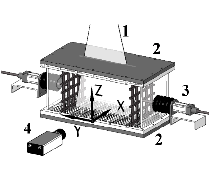
Figure 1: Experimental set-up: (1) -laser light sheet in $yz$ plane; (2) - heat exchangers; (3) - grid driver; (4) - digital CCD camera.

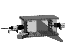
Figure 2: Experimental set-up with the laser light sheet in $xz$ plane.

In this section we describe the experimental set-up. The experiments in stably stratified turbulence have been conducted in rectangular chamber with dimensions $26\times 58\times 26$ cm³ in air flow with the Prandtl number Pr $=0.71$. The side walls of the chambers are made of transparent Perspex with the thickness of $1$ cm. In the experiments turbulence is produced by two oscillating grids. Pairs of vertically oriented grids with bars arranged in a square array (with a mesh size 5 cm) are attached to the right and left horizontal rods (see Figs. 1-3). The grids are positioned at a distance of two grid meshes from the chamber walls and are parallel to the side walls. Both grids are operated at the same amplitude of $3.05$ cm, at a random phase and at the same frequency which is varied in the range from $1$ Hz to $10.5$ Hz. To increase the size of the domain with a homogeneous turbulence and to decrease the mean velocity, vertical partitions were attached to the side walls of the chamber. We use the following system of coordinates: $z$ is the vertical axis, the $y$-axis is perpendicular to the grids and the $xz$-plane is parallel to the grids. The aspect ratio of the chamber $H_{y}/H_{z}=1.52$, where $H_{y}$ is the size of the chamber along $y$-axis between partitions and $H_{z}$ is the hight of the chamber, respectively.

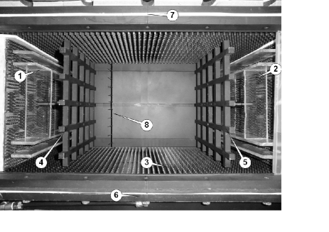
Figure 3: Rectangular chamber: (1,2) - partitions ; (3) - rectangular fins; (4,5) - oscillating grids; (6,7) - heat exchangers; (8) - temperature measurement system.

A vertical mean temperature gradient in the turbulent air flow was formed by attaching two aluminium heat exchangers to the bottom and top walls of the test section (a cooled bottom and a heated top wall of the chamber). To improve heat transfer in the boundary layers at the bottom and top walls we used heat exchangers with rectangular fins $0.3\times 0.3\times 1.5$ cm³ (see Fig. 3) which allowed us to form a mean temperature gradient up to 1.15 K/cm at a mean temperature of about 308 K when the frequency of the grid oscillations $f>10$ Hz. The thickness of the aluminium plates with the fins is 2.5 cm. The bottom plate is a top wall of the tank with cooling water. Temperature of water circulating through the tank and the chiller is kept constant within $0.1$ K. Cold water is pumped into the cooling system through two inlets and flows out through two outlets located at the side walls of the cooling system. The top plate is attached to the electrical heater that provides constant and uniform heating. The voltage applied to the heater varies up to 155 V. The power of the heater varies up to 300 W.

The temperature field was measured with a temperature probe equipped with twelve E-thermocouples (with the diameter of 0.013 cm and the sensitivity of $\approx 65\,\mu$V/K) attached to a vertical rod with a diameter 0.4 cm. The spacing between thermocouples along the rod was 2.2 cm. Each thermocouple was inserted into a 0.1 cm diameter and 4.5 cm long case. A tip of a thermocouple protruded at the length of 1.5 cm out of the case. The temperature in the central part of the chamber was measured for 2 rod positions in the horizontal and vertical directions, i.e., at 24 locations in a flow (see Fig. 3). The exact position of each thermocouple was measured using images captured with the optical system employed in PIV measurements. A sequence of 500 temperature readings for every thermocouple at every rod position was recorded and processed using the developed software based on LabView 7.0.

The velocity fields were measured using a Stereoscopic Particle Image Velocimetry (PIV), see Refs. AD91 ; RWK07 ; W00 . In the experiments we used LaVision Flow Master III system. A double-pulsed light sheet was provided by a Nd-YAG laser (Continuum Surelite $2\times 170$ mJ). The light sheet optics includes spherical and cylindrical Galilei telescopes with tuneable divergence and adjustable focus length. We used two progressive-scan 12 bit digital CCD cameras (with pixel size $6.7\,\mu$m $\times\,6.7\,\mu$m and $1280\times 1024$ pixels) with a dual-frame-technique for cross-correlation processing of captured images. A programmable Timing Unit (PC interface card) generated sequences of pulses to control the laser, camera and data acquisition rate. The software package LaVision DaVis 7 was applied to control all hardware components and for 32 bit image acquisition and visualization. This software package comprises PIV software for calculating the flow fields using cross-correlation analysis.

To obtain velocity maps in the central region of the flow in the cross-section parallel to the grids and perpendicular to a front view plane, we used one camera with a single-axis Scheimpflug adapter. The angle between the optical axis of the camera and the front view plane as well as the angle between the optical axis and the probed cross-section was approximately 45 degrees (see Fig. 2). The perspective distortion was compensated using Stereoscopic PIV system calibration kit whereby the correction was calculated for a recorded image of a calibration plate. The corrections were introduced in the probed cross-section images before their processing using a cross-correlation technique for determining velocity fields.

An incense smoke with sub-micron particles ($\rho_{p}/\rho\sim 10^{3})$, was used as a tracer for the PIV measurements. Smoke was produced by high temperature sublimation of solid incense grains. Analysis of smoke particles using a microscope (Nikon, Epiphot with an amplification of 560) and a PM-300 portable laser particulate analyzer showed that these particles have an approximately spherical shape and that their mean diameter is of the order of $0.7\mu$m. The probability density function of the particle size measured with the PM300 particulate analyzer was independent of the location in the flow for incense particle size of $0.5-1\,\mu$m. The maximum tracer particle displacement in the experiment was of the order of $1/4$ of the interrogation window. The average displacement of tracer particles was of the order of $2.5$ pixels. The average accuracy of the velocity measurements was of the order of $4\%$ for the accuracy of the correlation peak detection in the interrogation window of the order of $0.1$ pixel (see, e.g., Refs. AD91 ; RWK07 ; W00 ).

We determined the mean and the r.m.s. velocities, two-point correlation functions and an integral scale of turbulence from the measured velocity fields. Series of 520 pairs of images acquired with a frequency of 1 Hz, were stored for calculating velocity maps and for ensemble and spatial averaging of turbulence characteristics. The center of the measurement region in $yz$ and $xz$-planes coincides with the center of the chamber. We measured velocity in a flow domain $25.6\times 25.6$ cm² with a spatial resolution of $1024\times 1024$ pixels. This corresponds to a spatial resolution 250 $\mu$m / pixel. The velocity field in the probed region was analyzed with interrogation windows of $32\times 32$ or $16\times 16$ pixels. In every interrogation window a velocity vector was determined from which velocity maps comprising $32\times 32$ or $64\times 64$ vectors were constructed. The mean and r.m.s. velocities for every point of a velocity map were calculated by averaging over 520 independent maps, and then they were averaged over the central flow region.

The two-point correlation functions of the velocity field were determined for every point of the central part of the velocity map (with $16\times 16$ vectors) by averaging over 520 independent velocity maps, which yields 16 correlation functions in $x,y$ and $z$ directions. Then the two-point correlation function was obtained by averaging over the ensemble of these correlation functions. An integral scale of turbulence, $\ell$, was determined from the two-point correlation functions of the velocity field. In the experiments we evaluated the variability between the first and the last 20 velocity maps of the series of the measured velocity field. Since very small variability was found, these tests showed that 520 velocity maps contain enough data to obtain reliable statistical estimates. We found also that the measured mean velocity field is stationary.

The characteristic turbulence time in the experiments $\tau_{z}=0.2-1$ seconds that is much smaller than the time during which the velocity fields are measured $(520$ s). The size of the probed region did not affect our results. The temperature difference between the top and bottom plates, $\Delta\overline{T}$, in all experiments was 50 K.

IV Experimental results and comparison with the theoretical predictions

We will start with the discussion of the experimental results on the temperature measurements in stably stratified turbulent flows. To avoid side effects of the grids we present the experimental results recorded in the central region of the chamber with the size of $10\times 10\times 10$ cm³. The temperature was measured at 24 locations in a flow (the spacing between thermocouples was 2.2 cm). The separation distance of 2.2 cm between thermal couples is sufficient to measure the gradients of the mean temperature. Indeed, the integral scale of turbulence is about 2 cm (see below), and the characteristic length scale of the mean temperature field, $L_{T}=|\mbox{\boldmath$\nabla$}\overline{T}/\overline{T}|^{-1}$, is much larger than the integral scale of turbulence.

In our study we employ a triple decomposition whereby the instantaneous temperature $T^{tot}=T+\theta$, where $\theta$ are the temperature fluctuations and $T$ is the temperature determined by sliding averaging of the instantaneous temperature field over the time that is by one order of magnitude larger than the characteristic turbulence time (for the temperature difference between the top and bottom plates $\Delta\overline{T}=50$ K and the frequency $f=10.5$ Hz of the grid oscillations the sliding average time is 1.6 s, while the vertical turbulence time is 0.17 s). This temperature $T$ is given by a sum, $T=\overline{T}+\delta T$, where $\delta T$ are the long-term variations of the temperature $T$ due to the nonlinear temperature oscillations around the mean value $\overline{T}$. The mean temperature $\overline{T}$ is obtained by the additional averaging of the temperature $T$ over the time 400 s.

In the temperature measurements the acquisition frequency of the temperature was $1.25$ Hz. The corresponding acquisition time is $0.8$ s, that is larger than the characteristic turbulence time, $0.17$ s, and is much smaller than the period of non-linear oscillations of the mean temperature, $12$ s (see below). On the other hand, the time interval of the one realization of the temperature field is $400$ s, which corresponds to 500 data points of the temperature field over which we perform averaging. Therefore, the acquisition frequency of temperature is high enough to provide sufficiently long time series for statistical estimation of the mean temperature $\overline{T}$.

Let us now analyze the frequency dependence of vertical profiles of the mean temperature $\overline{T}(z)$ (Fig. 4). Inspection of Fig. 4 shows that the increase of the frequency $f$ of the grid oscillations weakly modifies the vertical profiles of the mean temperature $\overline{T}(z)$. However, the gradients of the mean temperature $\overline{T}$ in the vertical, $\nabla_{z}\overline{T}$, and horizontal, $\nabla_{y}\overline{T}$, directions are affected by the increase of the frequency $f$ of the grid oscillations (Fig. 5). In particular, the horizontal and vertical temperature gradients grow with the frequency of oscillation. The reasons for that will be explained in this section.

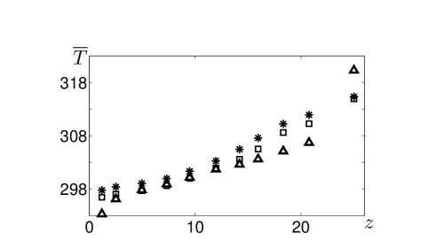
Figure 4: Vertical profile of the mean temperature $\overline{T}(z)$ for different frequencies $f$ of the grid oscillations for the stably stratified turbulent flow: $f=1$ Hz (triangles), $f=2$ Hz (squares), and $f=10.5$ Hz (snowflakes) for $\triangle\overline{T}=50$ K. The temperature is measured in K and the distance in cm.

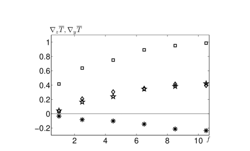
Figure 5: Vertical gradients of the mean temperature $\nabla_{z}\overline{T}$ (squares) and r.m.s. of $\delta(\nabla_{z}T)$ (diamonds) characterizing amplitude of the long-term nonlinear oscillations versus the frequency $f$ of the grid oscillations for the stably stratified turbulent flow for $\triangle\overline{T}=50$ K. Similar dependencies are also shown for horizontal gradients of the temperature $\nabla_{y}\overline{T}$ (snowflakes) and r.m.s. of $\delta(\nabla_{y}\overline{T})$ (stars). The temperature gradient is measured in K cm^-1 and the frequency $f$ is measured in Hz.

In the experiments we have observed the long-term nonlinear oscillations $\delta T$ of the temperature occurring around the mean temperature $\overline{T}$ with the periods which are much larger than the turbulent correlation time (see Fig. 6). In particular, in Fig. 6 we show time dependencies of the instantaneous (actual) temperature $T^{tot}=T+\theta$, the long-term variations of mean temperature $\delta T=T-\overline{T}$ and the long-term variations of the vertical mean temperature gradient $\delta(\nabla_{z}T)=\nabla_{z}T-\overline{\nabla_{z}T}$ due to the nonlinear oscillations of the mean temperature. We also determined the long-term variations of the mean temperature gradients $\delta(\nabla_{i}T)=\nabla_{i}T-\overline{\nabla_{i}T}$ in other directions, where $i=x,y,z$.

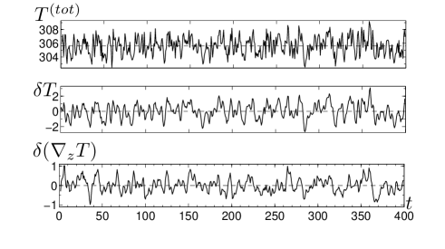
Figure 6: Time dependencies of the instantaneous temperature $T^{tot}=T+\theta$, the variations of mean temperature $\delta T=T-\overline{T}$ and the variations of the vertical mean temperature gradient $\delta(\nabla_{z}T)=\nabla_{z}T-\overline{\nabla_{z}T}$ due to the long-term nonlinear oscillations of the mean temperature (with the period $\sim 12$ s). These time dependencies are measured in the center of the chamber at the frequency $f=10.5$ Hz of the grid oscillations for the stably stratified turbulent flow for $\triangle\overline{T}=50$ K. These temperature characteristics are measured in K and time is measured in seconds.

In Fig. 7 we show the results of a Fourier analysis of the signal $\delta T=T-\overline{T}$. Inspection of Fig. 7 shows that there are two main maxima in the spectrum with the periods 12 s and 20 s. Other smaller maxima in the spectrum are at the frequencies which are multiples of these main frequencies or their sums and differences. These are typical features of nonlinear oscillations. The theory that explains the mechanism of these nonlinear oscillations of the mean temperature field, has not been developed yet. A possible mechanism for such nonlinear oscillations could be related to the large-scale Tollmien-Schlichting waves in sheared turbulent flows (see Ref. EGKR07 ).

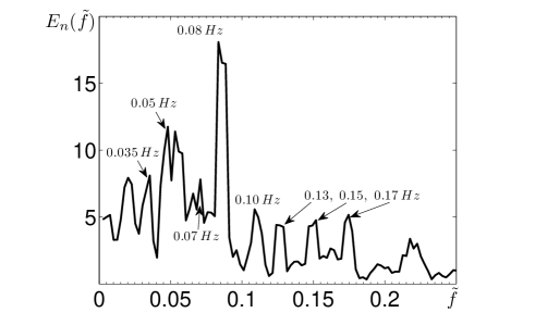
Figure 7: The normalized spectrum function $E_{n}(\tilde{f})=|(\delta T)_{\tilde{f}}|^{2}/\int|(\delta T)_{\tilde{f}}|^{2}\,d\tilde{f}$ of the signal $\delta T=T(t)-\overline{T}$, where in the Fourier space $(\delta T)_{\tilde{f}}=\int\delta T\,\exp[-i\tilde{f}\,t]\,dt$ and $\tilde{f}$ is the frequency of the nonlinear long-term oscillations of the mean temperature.

The results of our experiments in the stably stratified turbulence we will compare with the results obtained in the similar experimental set-up, but for the unstably stratified turbulence or for the isothermal turbulence when $\triangle\overline{T}=0$. The details of this experimental set-up and measurements are given in Ref.BEKR11 , in which the Rayleigh-Bénard apparatus with an additional source of turbulence produced by the two oscillating grids located nearby the side walls of the chamber was used. Additional forcing for turbulence allows to observe evolution of the mean temperature and velocity fields during the transition from turbulent convection with the large-scale circulations (LSC) for very small frequencies of the grid oscillations, to the limiting regime of unstably stratified flow without LSC for very high frequencies of the grid oscillations. In the latter case of the unstably stratified flow without LSC the temperature field behaves like a passive scalar.BEKR11

In our experiments with the stably stratified turbulence, we determined the dependence of the r.m.s. of the temperature fluctuations $\sqrt{\langle\theta^{2}\rangle}$ versus the frequency $f$ of the grid oscillations (see Fig. 8), where $\theta$ are fluctuations of fluid temperature. The temperature fluctuations monotonically increase with the increase of the frequency $f$ of the grid oscillations (except for the higher frequency) due to the monotonic increase of the mean temperature gradients. In the case of the unstably stratified turbulent flow the dependence $\sqrt{\langle\theta^{2}\rangle}$ versus frequency is more involved.

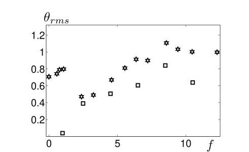
Figure 8: The r.m.s. of temperature fluctuations $\theta_{rms}=\sqrt{\langle\theta^{2}\rangle}$ versus the frequency $f$ of the grid oscillations for the stably (squares) and unstably (stars) stratified turbulent flows.

We also determined the frequency dependencies of the following measured turbulence parameters: the r.m.s. velocity fluctuations, $u_{\rm rms}=\left[\langle u_{x}^{2}+u_{y}^{2}+u_{z}^{2}\rangle\right]^{1/2}$ (Fig. 9), the vertical anisotropy $A_{z}=\langle u_{z}^{2}\rangle/u_{\rm rms}^{2}$ (Fig. 10), and the integral scales of turbulence along horizontal $y$ (Fig. 11) and vertical $z$ (Fig. 12) directions $(\ell_{y}$ and $\ell_{z})$. Except for the small frequencies of the grid oscillations, the horizontal integral scale of turbulence behaves similarly for both, the stably and unstably stratified turbulent flows, while the vertical integral scale of turbulence is systematically higher for the unstably stratified turbulent flow. On the other hand, the vertical anisotropy $A_{z}$ only slightly increases with the frequency of the grid oscillations.

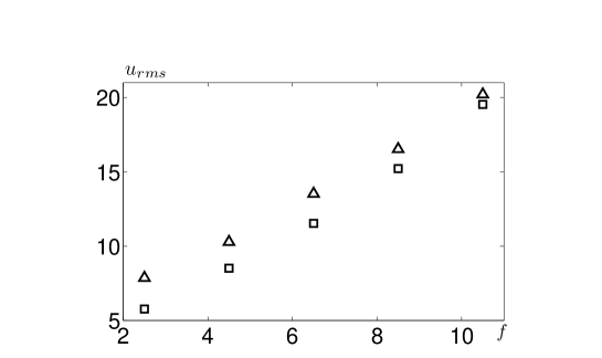
Figure 9: The r.m.s. turbulent velocity $u_{rms}$ versus frequency $f$ of the grid oscillations for the stably stratified turbulent flow with $\triangle\overline{T}=50$ K (squares) and for isothermal turbulence (triangles). The turbulent velocity is measured in cm s^-1 and the frequency $f$ is measured in Hz.

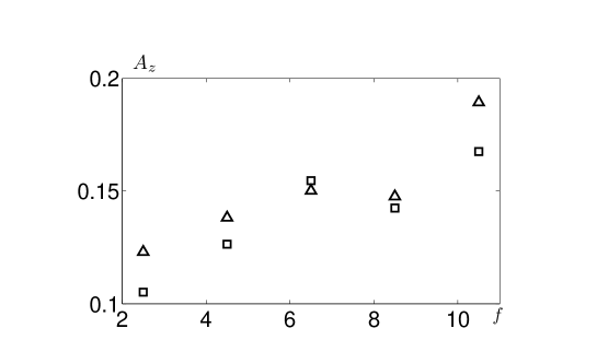
Figure 10: Vertical anisotropy $A_{z}=\langle u_{z}^{2}\rangle/u_{\rm rms}^{2}$ versus frequency $f$ of the grid oscillations for the stably stratified turbulent flow with $\triangle\overline{T}=50$ K (squares) and for isothermal turbulence (triangles).

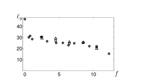
Figure 11: Horizontal integral scale of turbulence $\ell_{y}$ versus the frequency $f$ of the grid oscillations for the stably (squares) and unstably (stars) stratified turbulent flows with $\triangle\overline{T}=50$ K, and for isothermal turbulence (triangles). The turbulent length scales are measured in mm and the frequency $f$ is measured in Hz.

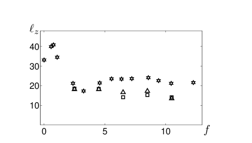
Figure 12: Vertical integral scale of turbulence $\ell_{z}$ versus the frequency $f$ of the grid oscillations for the stably (squares) and unstably (stars) stratified turbulent flows with $\triangle\overline{T}=50$ K, and for isothermal turbulence (triangles). The turbulent length scales are measured in mm and the frequency $f$ is measured in Hz.

Note that in the case of unstably stratified turbulent flow, a cutoff at the frequency of nearly 1.5 Hz is observed (see Figs. 8 and 11-12). At this frequency of the grid oscillations the large-scale coherent structures (convective cells) begin to break down due to the external forcing.

The two-point correlation functions of the velocity field have been calculated by averaging over 520 independent velocity maps (the time difference between the obtained velocity maps is by one order of magnitude larger than the turbulent time scales), and then they have been averaged over the central flow region. The integral scales of turbulence, $\ell_{y}$ and $\ell_{z}$, have been determined from the normalized two-point longitudinal correlation functions of the velocity field, e.g., $F_{y}(\tilde{y})=\langle u_{y}({\bf r}_{0})\,u_{y}({\bf r}_{0}+\tilde{y}\,{\bf e}_{y})\rangle/\langle u_{y}^{2}({\bf r}_{0})\rangle$ [and similarly for $F_{z}(\tilde{z})$ after replacing in the above formula $y$ by $z$], using the following expression: $\ell_{y}=\langle\int_{0}^{L}F_{y}(\tilde{y})\,d\tilde{y}\rangle_{S}$ [and similarly for $\ell_{z}$ after replacing in the above formula $y$ by $z$], where $L=10$ cm is the linear size of the probed flow region, ${\bf e}_{y}$ is the unit vector in the $y$ direction, and $\langle...\rangle_{S}$ is the additional averaging over the $yz$ cross-section of the probed region. Since the integral scales of turbulence, $\ell_{y}$ and $\ell_{z}$ are less than 3 cm, the size of the probed region, $L=10$ cm, is sufficiently large to assure a correct calculation of the integral scale of turbulence. We have checked that the increase of the size of the probed region, does not change the integral scales of turbulence.

In Fig. 13 we show the turbulent times, $\tau_{y}=\ell_{y}/\sqrt{\langle u_{y}^{2}\rangle}$ and $\tau_{z}=\ell_{z}/\sqrt{\langle u_{z}^{2}\rangle}$, along horizontal $y$ and vertical $z$ directions versus the frequency $f$ of the grid oscillations. When $f>3$ Hz, the the turbulent times along horizontal $y$ and vertical $z$ directions nearly coincide. In Fig. 14 we also show the rates of dissipation of the turbulent kinetic energies, $\varepsilon_{y}=\langle u_{y}^{2}\rangle^{3/2}/\ell_{y}$ and $\varepsilon_{z}=\langle u_{z}^{2}\rangle^{3/2}/\ell_{z}$, along horizontal $y$ and vertical $z$ directions versus the frequency $f$ of the grid oscillations. The difference in the rates of dissipation of the turbulent kinetic energies along horizontal $y$ and vertical $z$ directions increases with increase of the frequency $f$ of the grid oscillations. This is due to the fact that when the frequency $f$ increases, the horizontal turbulent velocity fluctuations increase faster than that in the vertical direction.

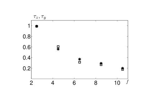
Figure 13: The turbulent times $\tau_{y}=\ell_{y}/\sqrt{\langle u_{y}^{2}\rangle}$ (snowflakes) and $\tau_{z}=\ell_{z}/\sqrt{\langle u_{z}^{2}\rangle}$ (squares) along horizontal $y$ and vertical $z$ directions versus the frequency $f$ of the grid oscillations for the stably stratified turbulent flow with $\triangle\overline{T}=50$ K. The turbulent times are measured in s and the frequency $f$ is measured in Hz.

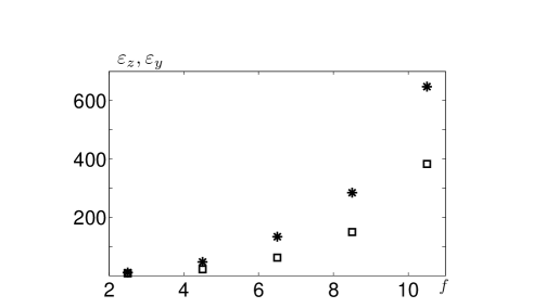
Figure 14: The rates of dissipation of the turbulent kinetic energies $\varepsilon_{y}=\langle u_{y}^{2}\rangle^{3/2}/\ell_{y}$ (snowflakes) and $\varepsilon_{z}=\langle u_{z}^{2}\rangle^{3/2}/\ell_{z}$ (squares) along horizontal $y$ and vertical $z$ directions versus the frequency $f$ of the grid oscillations for the stably stratified turbulent flow with $\triangle\overline{T}=50$ K. The rates of dissipation of the turbulent kinetic energies are measured in cm² s^-3 and the frequency $f$ is measured in Hz.

In Fig. 15 we show the Reynolds number $Re=\ell\,u_{rms}/\nu$ versus frequency of the grid oscillations for the stably stratified turbulent flow, where $\ell=(\ell_{x}^{2}+\ell_{y}^{2}+\ell_{z}^{2})^{1/2}$. The Reynolds number increases with the increase of the frequency of the grid oscillations due to increase of the production rate of turbulence. On the other hand, for the largest frequency $f$ the Reynolds number is independent of the stratification. This is because for the largest frequency $f$ of the grid oscillations the production of turbulence by the grid oscillations is much larger than suppression of the turbulence due to the buoyancy. We stress again that the parameters shown in Figs. 8-15, have been calculated by the spatial averaging over the central part of the chamber where the turbulent flow is nearly uniform.

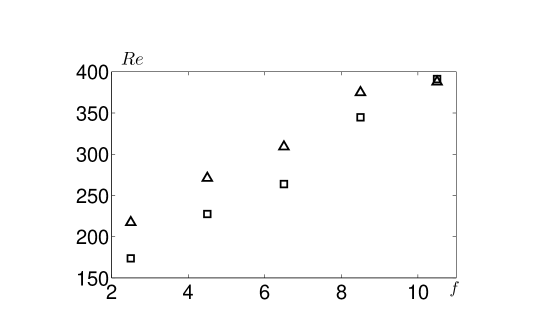
Figure 15: Reynolds number $Re=\ell\,u_{rms}/\nu$ versus frequency $f$ of the grid oscillations for the stably stratified turbulent flow for $\triangle\overline{T}=50$ K (squares) and for isothermal turbulence (triangles).

Now let us explain why the mean temperature gradients increase with the frequency $f$ of the grid oscillations (see Fig. 7). When the frequency $f$ of the grid oscillations increases, the fluctuations of velocity, $u_{\rm rms}$, and temperature, $\theta_{\rm rms}$, increase, while the integral scale of turbulence, $\ell$, decreases (see Figs. 8-9 and 11-12). This is the reason why the turbulent heat flux $(\propto u_{\rm rms}\,\theta_{\rm rms})$ increases faster than the turbulent diffusivity $(D^{T}\propto u_{\rm rms}\,\ell)$. Consequently, the mean temperature gradients $|\nabla_{i}\overline{T}|\sim|F_{i}|/D^{T}_{i}$, increase with the frequency $f$ of the grid oscillations.

In Fig. 16 we plot the non-dimensional ratio $\ell_{\ast}\,\nabla_{\ast}\overline{T}/\sqrt{\langle\theta^{2}\rangle}$ [see Eqs. (7) and (8)] versus the frequency $f$ of the grid oscillations for the stably stratified turbulent flow (squares) obtained in our experiments. For comparison in the same figure we show also this non-dimensional ratio obtained previouslyBEKR11 for the unstably stratified turbulent flow (stars). Inspection of Fig. 16 shows that this non-dimensional ratio is nearly independent of the frequency of the grid oscillations and has the same magnitude for both, stably and unstably stratified turbulent flows, in agreement with the theoretical predictions. Here we assumed that $\ell_{x}=\ell_{y}$, $C_{F}=0.2$ and $C_{\theta}=0.83$ for the unstably stratified turbulence, while $C_{\theta}=1.4$ for the stably stratified turbulence. Small deviations of the experimental results from the theoretical predictions [see Eq. (7)] may be caused by a non-zero term, ${\rm div}\,{\bf\Phi}_{\theta}$.

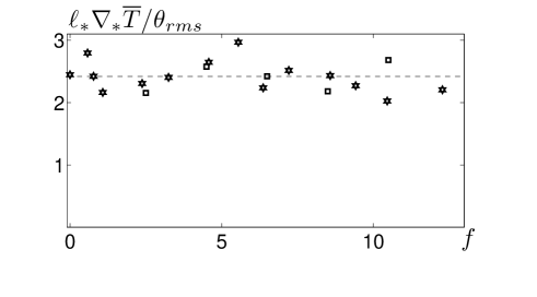
Figure 16: The non-dimensional ratio $\ell_{\ast}\,\nabla_{\ast}\overline{T}/\theta_{rms}$ versus the frequency $f$ of the grid oscillations for the stably (squares) and unstably (stars) stratified turbulent flows for $\triangle\overline{T}=50$ K, where $\theta_{rms}=\sqrt{\langle\theta^{2}\rangle}$.

Our measurements showed that $\tau_{y}=\tau_{z}$ (see Fig. 13), where $\tau_{i}=\ell_{i}/u_{i}$, and the deviation of the ratio $\tau_{z}/\tau_{x}$ from 1 is small. It should be noted also that the accuracy of the velocity measurements in the $x$ direction is probably less than in the $y,z$ directions, because of the use of Scheimpflug correction. In the theoretical estimates for simplicity we assumed that $\tau_{x}\approx\tau_{y}\approx\tau_{z}=\tau_{0}$. However, our main results [Eqs. (7)-(8)] are nearly independent of this assumption since main contributions to Eqs. (7)-(8) is from the term $\propto(\nabla_{z}\overline{T})^{2}$.

We also determined the frequency dependence of the ratio $u^{\ast}_{z}/u_{z}^{rms}$ (see Fig. 17), where $u_{z}^{rms}$ is the r.m.s. of the vertical component of velocity fluctuations in the stably stratified turbulent flow and $u^{\ast}_{z}$ is the r.m.s. of the vertical component of velocity fluctuations in the isothermal turbulence. We also determine the ratio $u_{z}^{\ast}/\tilde{u}_{z}$, where $\tilde{u}_{z}$ is the vertical component of the effective turbulent velocity, $\tilde{u}_{z}=[(u^{\ast}_{z})^{2}-C_{u}\ell_{z}\,\beta\,\sqrt{\langle\theta^{2}\rangle}]^{1/2}$. This effective velocity [see Eq. (11)] that takes into account the decay of the turbulence by buoyancy, is derived from the budget equation (9) for the vertical turbulent kinetic energy in Sect. II. Inspection of Fig. 17 shows that the values of these ratios, $u^{\ast}_{z}/u_{z}^{rms}$ and $u_{z}^{\ast}/\tilde{u}_{z}$, are very close. The latter implies that the measured turbulent velocity in the stably stratified turbulent flow, $u_{z}^{rms}$, is of the order of $\tilde{u}_{z}$, in agreement with the theoretical predictions.

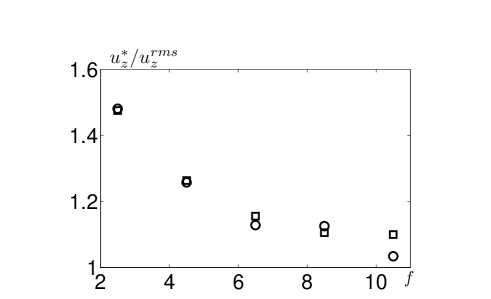
Figure 17: Ratios $u^{\ast}_{z}/u_{z}^{rms}$ (squares) and $u^{\ast}_{z}/\tilde{u}_{z}$ (circles) versus the frequency $f$ of the grid oscillations. Here $u_{z}^{rms}$ is the r.m.s. of the vertical component of velocity fluctuations in the stably stratified turbulent flow, $u^{\ast}_{z}$ is the r.m.s. of the vertical component of velocity fluctuations in the isothermal turbulence, $\tilde{u}_{z}$ is the vertical component of the effective turbulent velocity, $\tilde{u}_{z}=[(u^{\ast}_{z})^{2}-C_{u}\ell_{z}\,\beta\,\sqrt{\langle\theta^{2}\rangle}]^{1/2}$, that takes into account the attenuation of the turbulence by buoyancy. Here $C_{u}$ is an empirical constant that is about 1.81 for stably stratified turbulence and is about 4 for unstably stratified turbulence. The velocity is measured in cm s^-1 and the frequency $f$ is measured in Hz.

In our experiments the velocity and temperature fields are not acquired simultaneously. This may impair the accuracy of the estimates of the correlation coefficient $C$ in the vertical heat flux and the empirical constant $C_{u}$ in Eq. (11). However, in our experiments the turbulence is stationary in the statistical sense. Therefore, the estimates of the correlation coefficient $C$ and the empirical constant $C_{u}$ based on our experiments are reasonable.

To characterize the stably stratified flows, in Fig. 18 we show the turbulent Richardson number $Ri_{T}=N^{2}\tau_{0}^{2}$ versus frequency $f$ of the grid oscillations for the stably stratified turbulent flow, where $\tau_{0}=\ell/u_{rms}$ is the characteristic turbulent time. The turbulent Richardson number $Ri_{T}$ strongly decreases with the increase of the frequency of the grid oscillations due to the strong decrease of the turbulent correlation time $\tau_{0}$ with increase of the frequency $f$. For large frequencies of the grid oscillations whereby $Ri_{T}\ll 1$, the temperature field can be considered as a passive scalar.YW90 On the other hand, for smaller frequencies of the grid oscillations, $Ri_{T}>1$, and the temperature field behaves as an active field. Note that the passive-like scalar behaviour of the temperature field can be understood in the kinematic sense. In particular, when the temperature fluctuations $\langle\theta^{2}\rangle$ do not affect the turbulent kinetic energy, the temperature field can be considered as a passive scalar. This implies that the evolution of the temperature field in a given turbulent velocity field is a kinematic problem, whereby there is no dynamic coupling between the temperature fluctuations, $\langle\theta^{2}\rangle$, and the turbulent kinetic energy. When the effect of the temperature fluctuations on the turbulent kinetic energy cannot be neglected, the temperature is considered as an active field. This definition of the passive or active behavior of the temperature field is different from that based on the scaling behaviour of the temperature structure function. LX10

Figure 18: Turbulent Richardson number $Ri_{T}=N^{2}\tau_{0}^{2}$ versus frequency $f$ of the grid oscillations for the stably stratified turbulent flow.

V Conclusions

Temperature fluctuations in stably stratified forced turbulence in air flow are investigated in laboratory experiments. The stratification is caused by an imposed vertical temperature gradient, and the turbulence is sustained by vertical oscillating grids. We demonstrated that the ratio $\ell_{\ast}\,\nabla_{\ast}\overline{T}/\sqrt{\langle\theta^{2}\rangle}$ determined by Eq. (8), is nearly constant and is independent of the frequency of the grid oscillations in both, stably and unstably stratified turbulent flows. We also found that for large frequencies of the grid oscillations the turbulent Richardson number, $Ri_{T}$, is small and the temperature field can be considered as a passive scalar, while for smaller frequencies of the grid oscillations $(Ri_{T}>1)$ the temperature field behaves as an active field. The long-term nonlinear oscillations of the mean temperature in stably stratified turbulence have been observed for all frequencies of the grid oscillations similarly to the case of the unstably stratified flow. One of the explanations of this effect could be related to the large-scale Tollmien-Schlichting waves in sheared turbulent flowsEGKR07 , which can result in the nonlinear oscillations of the mean temperature field.

The temperature fluctuations have been investigated here also theoretically using the budget equations for turbulent kinetic energy, turbulent potential energy (determined by the temperature fluctuations) and turbulent heat flux. The developed theory is in a good agreement with the experimental results.

- (1) A. S. Monin and A. M. Yaglom, Statistical Fluid Mechanics (MIT Press, Cambridge, Massachusetts, 1971), Vol. 1.
- (2) S. Chandrasekhar, Hydrodynamic and Hydromagnetic Stability, (Dover Publications Inc., New York, 1961), Sect. 2.
- (3) J. Miles, “Richardson criterion for the stability of stratified shear-flow,” Phys. Fluids 29, 3470 (1986).
- (4) E. J. Strang and H. J. S. Fernando, “Vertical mixing and transports through a stratified shear layer,” J. Phys. Oceanogr. 31, 2026 (2001).
- (5) R. M. Banta, R. K. Newsom, J. K. Lundquist, Y. L. Pichugina, R. L. Coulter and L. Mahrt, “Nocturnal low-level jet characteristics over Kansas during CASES-99,” Boundary-Layer Meteorol. 105, 221 (2002).
- (6) E. R. Pardyjak, P. Monti and H. J. S. Fernando, “Flux Richardson number measurements in stable atmospheric shear flows,” J. Fluid Mech. 459, 307 (2002).
- (7) P. Monti, H. J. S. Fernando, M. Princevac, W. C. Chan, T. A. Kowalewski and E. R. Pardyjak, “Observations of flow and turbulence in the nocturnal boundary layer over a slope,” J. Atmos. Sci. 59, 2513 (2002).
- (8) J. S. Lawrence, M. C. B. Ashley, A. Tokovinin and T. Travouillon, “Exceptional astronomical seeing conditions above Dome C in Antarctica,” Nature 431, 278 (2004).
- (9) L. F. Richardson, “The supply of energy from and to atmospheric eddies,” Pros. Roy. Soc. London A 97, 354 (1920).
- (10) E. N. Lorenz, The Nature and the Theory of the General Circulation of the Atmosphere (World Meteorological Organisation, Geneva, 1967).
- (11) T. Elperin, N. Kleeorin, I. Rogachevskii and S. Zilitinkevich, “New Turbulence Closure Equations for Stable Boundary Layer: Return to Kolmogorov (1941),” 5th Annual Meeting of the European Meteorological Society, paper No. 0553 (Utrecht, Netherlands, 2005).
- (12) S. S. Zilitinkevich, T. Elperin, N. Kleeorin and I. Rogachevskii, “Energy- and flux budget (EFB) turbulence closure model for stably stratified flows. Part I: Steady-state, homogeneous regimes,” Boundary-Layer Meteorol. 125, 167 (2007).
- (13) S. S. Zilitinkevich, T. Elperin, N. Kleeorin, I. Rogachevskii, I. Esau, T. Mauritsen and M. Miles, “Turbulence energetics in stably stratified geophysical flows: strong and weak mixing regimes,” Quart. J. Roy. Met. Soc. 134, 793 (2008).
- (14) S. S. Zilitinkevich, T. Elperin, N. Kleeorin, V. L’vov and I. Rogachevskii, “Energy- and flux-budget turbulence closure model for stably stratified flows. Part II: the role of internal gravity waves,” Boundary-Layer Meteorol. 133, 139 (2009).
- (15) S. S. Zilitinkevich, T. Elperin, N. Kleeorin, I. Rogachevskii, and I. Esau, “A hierarchy of energy- and flux-budget (EFB) turbulence closure models for stably stratified geophysical flows,” Boundary-Layer Meteorology, in press (2012), e-print, ArXiv: 1110.4994.
- (16) L. A. Ostrovsky and Yu. I. Troitskaya, “A model of turbulent transfer and dynamics of turbulence in a stratified shear flow,” Izvestiya AN SSSR FAO 23, 1031 (1987).
- (17) J. S. Turner, Buoyancy Effects in Fluids (Cambridge University Press, Cambridge, 1973).
- (18) G. Holloway, “Consideration on the theory of temperature spectra in stably stratified turbulence,” J. Phys. Oceonography 16, 2179 (1986).
- (19) V. M. Canuto and F. Minotti, “Stratified turbulence in the atmosphere and oceans: a new sub-grid model,” J. Atmos. Sci. 50, 1925 (1993).
- (20) U. Schumann and T. Gerz, “Turbulent mixing in stably stratified sheared flows,” J. Appl. Meteorol. 34, 33 (1995).
- (21) K. Keller and C. W. Van Atta, “An experimental investigation of the vertical temperature structure of homogeneous stratified shear turbulence,” J. Fluid Mech. 425, 1 (2000).
- (22) P. J. Luyten, S. Carniel and G. Umgiesser, “Validation of turbulence closure parameterisations for stably stratified flows using the PROVESS turbulence measurements in the North Sea,” J. Sea Research 47, 239 (2002).
- (23) S. S. Zilitinkevich, “Third-order transport due to internal waves and non-local turbulence in the stably stratified surface layer,” Quart. J. Roy. Meteorol. Soc. 128, 913 (2002).
- (24) L. H. Jin, R. M. C. So and T. B. Gatski, “Equilibrium states of turbulent homogeneous buoyant flows,” J. Fluid Mech. 482, 207 (2003).
- (25) H. Hanazaki and J. C. R. Hunt, “Structure of unsteady stably stratified turbulence with mean shear,” J. Fluid Mech. 507, 1 (2004).
- (26) L. Umlauf, “Modelling the effects of horizontal and vertical shear in stratified turbulent flows,” Deep-Sea Research 52, 1181 (2005).
- (27) C. R. Rehmann and J. H. Hwang, “Small-scale structure of strongly stratified turbulence,” J. Phys. Oceanogr. 32, 154 (2005).
- (28) T. Mauritsen, G. Svensson, S. S. Zilitinkevich, I. Esau, L. Enger and B. Grisogono, “A total turbulent energy closure model for neutrally and stably stratified atmospheric boundary layers,” J. Atmos. Sci. 64, 4117 (2007).
- (29) V. S. L’vov, I. Procaccia and O. Rudenko, “Turbulent fluxes in stably stratified boundary layers,” Physica Scripta T132, 014010 (2008).
- (30) V. S. L’vov and O. Rudenko, “Equations of motion and conservation laws in a theory of stably stratified turbulence,” Physica Scripta T132, 014009 (2008).
- (31) V. M. Canuto, “Turbulence in astrophysical and geophysical flows,” Lect. Notes Phys. 756, 107 (2009).
- (32) V. M. Canuto, Y. Cheng, A. M. Howard and I. N. Esau, “Stably stratified flows: A model with no Ri(cr),” J. Atmos. Sci. 65, 2437 (2008).
- (33) M. Bukai, A. Eidelman, T. Elperin, N. Kleeorin, I. Rogachevskii and I. Sapir-Katiraie, “Transition phenomena in unstably stratified turbulent flows,” Phys. Rev. E 83, 036302 (2011).
- (34) A. Eidelman, T. Elperin, N. Kleeorin, A. Markovich and I. Rogachevskii, “Hysteresis phenomenon in turbulent convection,” Experim. Fluids 40, 723 (2006).
- (35) J. Buchholz, A. Eidelman, T. Elperin, G. Grünefeld, N. Kleeorin, A. Krein, I. Rogachevskii, “Experimental study of turbulent thermal diffusion in oscillating grids turbulence,” Experim. Fluids 36, 879 (2004).
- (36) A. Eidelman, T. Elperin, N. Kleeorin, A. Krein, I. Rogachevskii, J. Buchholz, G. Grünefeld, “Turbulent thermal diffusion of aerosols in geophysics and in laboratory experiments,” Nonl. Proc. Geophys. 11, 343 (2004).
- (37) A. Eidelman, T. Elperin, N. Kleeorin, I. Rogachevskii and I. Sapir-Katiraie, “Turbulent thermal diffusion in a multi-fan turbulence generator with the imposed mean temperature gradient,” Experim. Fluids 40, 744 (2006).
- (38) A. Eidelman, T. Elperin, N. Kleeorin, A. Markovich and I. Rogachevskii, “Experimental detection of turbulent thermal diffusion of aerosols in non-isothermal flows,” Nonl. Proc. Geophys. 13, 109 (2006).
- (39) A. Eidelman, T. Elperin, N. Kleeorin, B. Melnik and I. Rogachevskii, “Tangling clustering of inertial particles in stably stratified turbulence,” Phys. Rev. E 81, 056313 (2010).
- (40) T. Elperin, N. Kleeorin and I. Rogachevskii, “Turbulent thermal diffusion of small inertial particles,” Phys. Rev. Lett. 76, 224 (1996).
- (41) T. Elperin, N. Kleeorin and I. Rogachevskii, “Turbulent barodiffusion, turbulent thermal diffusion and large-scale instability in gases,” Phys. Rev. E 55, 2713 (1997).
- (42) J. C. Kaimal and J. J. Fennigan, Atmospheric Boundary Layer Flows (Oxford University Press, New York, 1994).
- (43) Y. Cheng, V. M. Canuto and A. M. Howard, J., “An improved model for the turbulent PBL,” Atmosph. Sci. 59, 1550 (2002).
- (44) A. S. Monin and A. M. Yaglom, Statistical Fluid Mechanics (MIT Press, Cambridge, Massachusetts, 1975), Vol. 2.
- (45) W. D. McComb, The Physics of Fluid Turbulence (Clarendon, Oxford, 1990).
- (46) J. C. Rotta, “Statistische theorie nichthomogener turbulenz,” Z. Physik 129, 547 (1951).
- (47) R. J. Adrian, “Particle-imaging tecniques for experimental fluid mechanics,” Annu. Rev. Fluid Mech. 23, 261 (1991).
- (48) J. Westerweel, “Theoretical analysis of the measurement precision in particle image velocimetry,” Exper. Fluids 29, S3-12 (2000).
- (49) C. Raffel, C. Willert, S. Werely and J. Kompenhans, Particle Image Velocimetry, (Springer, Berlin-Heidelberg, 2007).
- (50) T. Elperin, I. Golubev, N. Kleeorin and I. Rogachevskii, “Large-scale instability in a sheared turbulence: formation of vortical structuress,” Phys. Rev. E 76, 066310 (2007).
- (51) K. Yoon and Z. Warhaft, “The evolution of grid-generated turbulence under conditions of stable thermal stratification,” J. Fluid Mech. 215, 601 (1990).
- (52) D. Lohse and K.-Q. Xia, “Small-scale properties of turbulent Rayleigh-Bénard Convection,” Annu. Rev. Fluid Mech. 42, 335 (2010).